


1. Introduction
Calculation of Feynman integrals at the multi-loop level is of great importance for both perturbation quantum field theory and particle experiments. The general strategy is to expand arbitrary integrals to finite simpler integrals (called Master Integrals) and then do the integration of master integrals only. Thus, tensor reduction of Feynman integrals is one of the critical steps for various realistic calculations in the Standard Model. There is a large body of research on one-loop reduction [1–25]. For reducing multi-loop integrals, various ideas and methods have been developed. There are some works on two-loop tensor reduction for some special integrals [26–31], while an algorithm for the reduction of general Feynman integrals was proposed in [32–37]. Among these methods, the Integration-By-Parts (IBP) method [36, 37] is widely used and has been implemented by some powerful programs such as FIRE, LiteRed, Kira, etc [38–45]. Although its popularity, the number of IBP identities grows very fast with the increasing number of mass scalars and higher rank of tensor structure, it will become a bottleneck when dealing with complicated physical processes. Even at the one-loop level, reducing a general tensor massive pentagon with the IBP method is difficult. Thus it is always welcome to find a more efficient reduction method.
PV-reduction [3] for one-loop integrals has played a significant role in general one-loop computations in history. However, when trying to generalize the method to higher loops, it becomes hard, and there are not many works in the literature. In [26, 46], the tensor two-loop integrals with only two external legs are reduced to scalar integrals with the PV-reduction method. However, an extra massless propagator appears. Integrals with new topologies have been introduced as master integrals to address the problem. This results against the intuitive picture: Reduction is achieved by removing one or more propagators from the original topology. Thus the reduction and master integrals should be constrained to the original topology and its sub-topologies.
Recently, we have generalized the original PV-reduction method for one-loop integrals by introducing an auxiliary vector R in [47, 48]. Our improved PV-reduction method can be easily carried out and compute reduction coefficients analytically by employing algebraic recursion relations. With these analytical expressions, one can do many things. For example, by taking limits properly, we can solve the reduction with propagators having general higher powers [49]. When external momenta are not general, i.e., the Gram determinant becomes zero, master integrals in the basis will not be independent anymore. We can systematically study their degeneration [50].
Encouraged by the results in [47, 48], we want to see if such an improved PV-reduction method can be transplanted to higher loops. When moving to two loops, some complexities arise. The first is that we need to determine the master integrals. For one-loop, the master integrals are trivially known. For higher loops, the choice of master integrals becomes an art. With proper choice, one can reduce the computation greatly [51]. The second is that when intuitively generalizing our method to two loops, we will meet the irreducible scalar products, which cannot be reduced. In fact, these two complexities are related to each other. To avoid unnecessary complexity, we will focus on the simplest nontrivial two-loop integrals, i.e., the sunset topology in this paper. With this example, we will show how to generalize our new PV-reduction method to two loops.
This paper is structured as follows. In section 2 , we briefly review our previous work on one-loop tensor reduction and discuss the main idea for the reduction of sunset integrals. In section 3 , we derive recursion relations for sunset integrals using differential operators and the proper choice of the master integrals in our algorithm. In section 4 , we demonstrate our algorithm successfully to sunset integrals with the total rank from one to four. In section 5 , we give some discussions and the plan for further studying. Technical details are collected in the appendix .
2. Brief discussion of tensor reduction with auxiliary vector
In this section, we will give a brief discussion of the general idea of using the auxiliary vector R to do tensor reduction. We first review the method presented in [47, 48] and then move to the two-loop sunset integrals. For the tensor reduction of a general one-loop integral (to avoid confusion, we denote Pj as propagators for one-loop integrals while Dj for two-loop integrals)${R}_{i,{\mu }_{i}}$ . Furthermore, we can combine these Ri to $R={\sum }_{i=1}^{m}{x}_{i}{R}_{i}$ to simplify the expression (2.1 ) to
$\begin{eqnarray}{I}_{n+1}^{{\mu }_{1}{\mu }_{2}\cdots {\mu }_{m}}\equiv \int \displaystyle \frac{{{\rm{d}}}^{D}{\ell }}{{\rm{i}}{\pi }^{D/2}}\displaystyle \frac{{{\ell }}^{{\mu }_{1}}{{\ell }}^{{\mu }_{2}}...{{\ell }}^{{\mu }_{m}}}{{P}_{0}{\prod }_{j=1}^{n-1}{P}_{j}}=\int \displaystyle \frac{{{\rm{d}}}^{D}{\ell }}{{\rm{i}}{\pi }^{D/2}}\displaystyle \frac{{{\ell }}^{{\mu }_{1}}{{\ell }}^{{\mu }_{2}}...{{\ell }}^{{\mu }_{m}}}{({{\ell }}^{2}-{M}_{0}^{2}){\prod }_{j=1}^{n}({\left({\ell }-{K}_{j}\right)}^{2}-{M}_{j}^{2})},\end{eqnarray}$
one can recover its tensor structure by multiplying each index with an auxiliary vector $\begin{eqnarray}{I}_{n+1}^{(m)}\equiv \int \displaystyle \frac{{{\rm{d}}}^{D}{\ell }}{{\rm{i}}{\pi }^{D/2}}\displaystyle \frac{{\left(2R\cdot {\ell }\right)}^{m}}{{P}_{0}{\prod }_{j=1}^{n}{P}_{j}}.\end{eqnarray}$
The good point of using (2.2 ) instead of (2.1 ) is that we have avoided the complicated Lorentz tensor structure in the reduction process, while they can easily be retained using the expansion of R and taking corresponding coefficients of xi's. Since we are using dimensional regularization, we like to keep the D as a general parameter. For D = d − 2ε, the master basis is the scalar integrals with n ≤ d + 1 propagators, i.e., the reduction results can be written as${I}_{n;\widehat{{i}_{1},\ldots ,{i}_{a}}}$ as the integrals got by removing propagators ${P}_{{i}_{1}},{P}_{{i}_{2}},\ldots ,{P}_{{i}_{a}}$ from In. For simplicity, we denote
$\begin{eqnarray}{I}_{n}^{(m)}={C}_{n\to n}^{(m)}{I}_{n}+{C}_{n\to n;\widehat{i}}^{(m)}{I}_{n;\widehat{i}}+{C}_{n\to n;\widehat{{ij}}}^{(m)}{I}_{n;\widehat{{ij}}}+\ldots \end{eqnarray}$
where we denote $\begin{eqnarray}{s}_{{ij}}\equiv {K}_{i}\cdot {K}_{j},\,\,\,{s}_{0i}\equiv R\cdot {K}_{i},\ \ {f}_{i}\equiv {M}_{0}^{2}-{M}_{i}^{2}+{s}_{{ii}}.\end{eqnarray}$
By the explicit permutation symmetry in (2.1 ), we only need to calculate ${C}_{n+1\to \{0,1,\ldots ,r\}}^{(m)}\equiv {C}_{n+1\to n+1;\widehat{r+1},\widehat{r+2},\ldots ,\widehat{n}}^{(m)}$ while other reduction coefficients can be got by proper replacements and momentum shifting. With the introduction of auxiliary vector R in (2.2 ), one can expand the reduction coefficients according to their tensor structure${{ \mathcal D }}_{i}\equiv {K}_{i}\cdot \displaystyle \frac{\partial }{\partial R}$ and ${ \mathcal T }\equiv {\eta }^{\mu \nu }\displaystyle \frac{\partial }{\partial {R}^{\mu }}\displaystyle \frac{\partial }{\partial {R}^{\nu }}$ on (2.2 ), we get the recursion relations for the expansion coefficients ${c}_{{a}_{1},\cdots ,{a}_{n}}^{(0,1,\cdots ,r)}$ $\widetilde{{\boldsymbol{G}}}=\left\{\displaystyle \frac{{s}_{{ij}}}{{M}_{0}^{2}}\right\}$ is the n × n rescaled Gram matrix and T = diag(a1 + 1, a2 + 1, ⋯ ,an + 1) is a diagonal matrix. The vectors in the equations (2.6 ) and (2.7 ) are defined as${\widehat{a}}_{i}$ indicates to drop the index ai. With the known boundary conditions, one can obtain all reduction coefficients by applying the recursions (2.6 ) and (2.7 ) iteratively.
$\begin{eqnarray}{C}_{n+1\to \{0,1,\ldots ,r\}}^{(m)}=\sum _{2{a}_{0}+{\sum }_{k=1}^{n}{a}_{k}=m}\left\{{c}_{{a}_{1},\cdots ,{a}_{n}}^{(0,1,\cdots ,r)}(m){\left({M}_{0}^{2}\right)}^{{a}_{0}+r-n}{\prod }_{k=0}^{n}{s}_{0k}^{{a}_{k}}\right\}.\end{eqnarray}$
By acting two types of differential operators $\begin{eqnarray}{{\boldsymbol{c}}}^{(\mathrm{0,1},\cdots ,r)}({a}_{1},\cdots ,{a}_{n};m)={{\boldsymbol{T}}}^{-1}{\widetilde{{\boldsymbol{G}}}}^{-1}{{\boldsymbol{O}}}^{(\mathrm{0,1},\cdots ,r)}({a}_{1},\cdots ,{a}_{n};m),\end{eqnarray}$
$\begin{eqnarray}{c}_{{\underbrace{0,\cdots ,0}}_{{\rm{n}}\ \mathrm{times}}}^{(0,1,\cdots ,r)}(2k)=\displaystyle \frac{2k-1}{D+2k-n-2}\left[(4-{{\boldsymbol{\alpha }}}^{{\rm{T}}}{\widetilde{{\boldsymbol{G}}}}^{-1}{\boldsymbol{\alpha }}){c}_{{\underbrace{0,\cdots ,0}}_{{\rm{n}}\ \mathrm{times}}}^{(0,1,\cdots ,r)}(2k-2)+{{\boldsymbol{\alpha }}}^{{\rm{T}}}{\widetilde{{\boldsymbol{G}}}}^{-1}{{\boldsymbol{c}}}_{{\underbrace{0,\cdots ,0}}_{{\rm{n}}-1\ \mathrm{times}}}^{(0,1,\cdots ,r)}(2k-2)\right],\end{eqnarray}$
where $\begin{eqnarray}\alpha \equiv \left(\displaystyle \frac{{f}_{1}}{{M}_{0}^{2}},\displaystyle \frac{{f}_{2}}{{M}_{0}^{2}},\cdots ,\displaystyle \frac{{f}_{n}}{{M}_{0}^{2}}\right),\ {\left[{{\boldsymbol{c}}}^{(\mathrm{0,1},\cdots ,r)}({a}_{1},\cdots ,{a}_{n};m)\right]}_{i}\equiv {c}_{{a}_{1},{a}_{2},\cdots ,{a}_{i}+1,\cdots ,{a}_{n}}^{(0,1,\cdots ,r)}(m),\end{eqnarray}$
and $\begin{eqnarray}\begin{array}{l}{\left[{{\boldsymbol{O}}}^{(\mathrm{0,1},\cdots ,r)}({a}_{1},\cdots ,{a}_{n};m)\right]}_{i}\equiv m{\alpha }_{i}{c}_{{a}_{1},\cdots ,{a}_{n}}^{(0,1,\cdots ,r)}(m-1)-m{\delta }_{0{a}_{i}}{c}_{{a}_{1},\cdots ,{\widehat{a}}_{i},\cdots ,{a}_{n}}^{(0,1,\cdots ,r)}(m-1;\widehat{i})\\ -(m+1-\displaystyle \sum _{l=1}^{n}{a}_{l}){c}_{{a}_{1},\cdots ,{a}_{i}-1,{a}_{i},\cdots ,{a}_{n}}^{(0,1,\cdots ,r)}(m),\\ {{\boldsymbol{c}}}_{\mathop{\underbrace{0,\cdots ,0}}\limits_{{\rm{n}}-1\ \mathrm{times}}}^{(0,1,\cdots ,r)}(m)\equiv \left(0,0,\cdots ,0,{c}_{\mathop{\underbrace{0,\cdots ,0}}\limits_{{\rm{n}}-1\ \mathrm{times}}}^{(0,1,\cdots ,r)}(m;\widehat{r+1}),\cdots ,{c}_{\mathop{\underbrace{0,\cdots ,0}}\limits_{{\rm{n}}-1\ \mathrm{times}}}^{(0,1,\cdots ,r)}(m;\widehat{n})\right).\end{array}\end{eqnarray}$
where One important point of the above reduction method is that we need to use both ${{ \mathcal D }}_{i}$ and ${ \mathcal T }$ operators to completely fix unknown coefficients in (2.5 ). One simple explanation is that in (2.5 ) coefficients there are (n + 1) indices (ai, i = 1,…,n and rank m), so naively (n + 1) relations are needed. A more accurate explanation is a little tricky. Let us take the bubble, i.e., n = 1 as an example. As shown in table 1, for rank m, there are ${N}_{c}=\left(\lfloor \tfrac{m}{2}\rfloor +1\right)$ unknown coefficients while the number of independent ${ \mathcal D }$ -type equations is ${N}_{{ \mathcal D }}=\lfloor \tfrac{m+1}{2}\rfloor $ . Thus, only using the ${ \mathcal D }$ -type operators we can fix all coefficients with odd rank m = (2k + 1) by these known terms with lower rank m ≤ 2k. However, for m = 2k + 2, ${N}_{c}-{N}_{{ \mathcal D }}=1$ , thus just using ${ \mathcal D }$ -type relations is not enough and we need to adopt the ${ \mathcal T }$ operator to provide one extra independent relation. In fact, ${ \mathcal T }$ provides more than just one relation, but other relations are not independent to these coming from ${ \mathcal D }$ and can be taken as the consistent check of the reduction method.
Table 1. Number of expansion coefficients and independent equations for tensor bubble. |
| Rank m | Nc | | | |
|---|---|---|---|---|
| 1 | 1 | 1 | 1 | 0 |
| 2 | 2 | 1 | 2 | 0 |
| 3 | 2 | 2 | 2 | 0 |
| 4 | 3 | 2 | 3 | 0 |
| 5 | 3 | 3 | 3 | 0 |
| 6 | 4 | 3 | 4 | 0 |
In this paper, we want to generalize our reduction method from one-loop to two-loop integrals. Again, with a simplified tensor structure, we define the general tensor integrals of sunset topology as5(5For simplicity, we denote the scalar integral ${I}_{{a}_{1},{a}_{2},{a}_{3}}\equiv {I}_{{a}_{1},{a}_{2},{a}_{3}}^{(0,0)}$ .)
$\begin{eqnarray}{I}_{{a}_{1},{a}_{2},{a}_{3}}^{({r}_{1},{r}_{2})}\equiv \int \displaystyle \frac{{{\rm{d}}}^{D}{{\ell }}_{1}}{{\rm{i}}{\pi }^{D/2}}\displaystyle \frac{{{\rm{d}}}^{D}{{\ell }}_{2}}{{\rm{i}}{\pi }^{D/2}}\displaystyle \frac{{\left(2{{\ell }}_{1}\cdot {R}_{1}\right)}^{{r}_{1}}{\left(2{{\ell }}_{2}\cdot {R}_{2}\right)}^{{r}_{2}}}{{D}_{1}^{{a}_{1}}{D}_{2}^{{a}_{2}}{D}_{3}^{{a}_{3}}.}\end{eqnarray}$
where the propagators are $\begin{eqnarray}{D}_{1}\equiv {{\ell }}_{1}^{2}-{M}_{1}^{2},\,\,\,{D}_{2}\equiv {{\ell }}_{2}^{2}-{M}_{2}^{2},\,\,\,\,{D}_{3}\equiv {\left({{\ell }}_{1}+{{\ell }}_{2}-K\right)}^{2}-{M}_{3}^{2}.\end{eqnarray}$
In this paper, we consider only the reduction with all ai = 1. For ai ≥ 2, one can use the same strategy presented in [49]. For simplicity, we denote2.13 ), the expansion coefficients ${\vec{\alpha }}_{{i}_{1},{i}_{2},j}^{({r}_{1},{r}_{2})}$ are actually vectors with components corresponding to different master integrals Ji. The summation over indices {i1, i2, j} ≥ 0 admits to the restriction $0\leqslant ({r}_{l}-{i}_{l}-j)/2\in {\mathbb{N}},l\,=\,1,2$ . We make the indices free by setting all ${\vec{\alpha }}_{{i}_{1},{i}_{2},j}^{({r}_{1},{r}_{2})}=0$ for inappropriate indices throughout the paper, so we will drop the prime in other summations. Similar to the strategy for one-loop case, we solve expansion coefficients from lower rank levels to higher rank levels iteratively, where the rank level is defined as the total rank (r1 + r2).
$\begin{eqnarray}\int {\rm{d}}{\ell }_{i}(\bullet )\equiv \int \displaystyle \frac{{{\rm{d}}}^{D}{\ell }_{i}}{{\rm{i}}{\pi }^{D/2}}(\bullet ),\,\,\,\,\int {\rm{d}}{\ell }_{1,2}(\bullet )\equiv \int \displaystyle \frac{{{\rm{d}}}^{D}{\ell }_{1}}{{\rm{i}}{\pi }^{D/2}}\displaystyle \frac{{{\rm{d}}}^{D}{\ell }_{2}}{{\rm{i}}{\pi }^{D/2}}(\bullet )={\int }_{1,2}(\bullet ).\end{eqnarray}$
Similar to what we do for one-loop case, we can expand reduction coefficients according to their tensor structure6 $\begin{eqnarray}{I}_{1,1,1}^{({r}_{1},{r}_{2})}={{\boldsymbol{C}}}^{({r}_{1},{r}_{2})}{\boldsymbol{J}}=\displaystyle \sum _{{i}_{1},{i}_{2},j}^{{\prime} }{s}_{01}^{{i}_{1}}{s}_{0^{\prime} 1}^{{i}_{2}}{s}_{00^{\prime} }^{j}{s}_{00}^{\displaystyle \frac{{r}_{1}-{i}_{1}-j}{2}}{s}_{0^{\prime} 0^{\prime} }^{\displaystyle \frac{{r}_{2}-{i}_{2}-j}{2}}{\vec{\alpha }}_{{i}_{1},{i}_{2},j}^{({r}_{1},{r}_{2})}\,{\boldsymbol{J}}\end{eqnarray}$
where we have written C, J to emphasize they are vector, while other kinematic variables are $\begin{eqnarray}{s}_{01}={R}_{1}\cdot K,\,\,{s}_{0^{\prime} 1}={R}_{2}\cdot K,\,\,{s}_{11}={K}^{2},\,\,{s}_{00}={R}_{1}^{2},\,\,{s}_{0^{\prime} 0^{\prime} }={R}_{2}^{2},\,\,\,{s}_{00^{\prime} }={R}_{1}\cdot {R}_{2}.\end{eqnarray}$
In (When we do the tensor reduction, we will reach the sub-topologies where one of the propagators in (2.11 ) is removed. For these cases, the integrals are reduced to the product of two one-loop tadpoles. Their tensor reduction has been solved in appendix B . To simplify notation, we denote
$\begin{eqnarray}{I}_{1,1,1;\hat{i}}^{({r}_{1},{r}_{2})}\equiv \int \displaystyle \frac{{{\rm{d}}}^{D}{\ell }_{1}}{{\rm{i}}{\pi }^{D/2}}\displaystyle \frac{{{\rm{d}}}^{D}{\ell }_{2}}{{\rm{i}}{\pi }^{D/2}}\displaystyle \frac{{\left(2{\ell }_{1}\cdot {R}_{1}\right)}^{{r}_{1}}{\left(2{\ell }_{2}\cdot {R}_{2}\right)}^{{r}_{2}}{D}_{i}}{{D}_{1}{D}_{2}{D}_{3}}\end{eqnarray}$
and their reductions are written as $\begin{eqnarray}{I}_{1,1,1;\widehat{i}}^{({r}_{1},{r}_{2})}={{\bf{C}}}_{\widehat{i}}^{({r}_{1},{r}_{2})}{\bf{J}}=\sum _{{i}_{1},{i}_{2},j}{s}_{01}^{{i}_{1}}{s}_{0^{\prime} 1}^{{i}_{2}}{s}_{00^{\prime} }^{j}{s}_{00}^{\displaystyle \frac{{r}_{1}-{i}_{1}-j}{2}}{s}_{0^{\prime} 0^{\prime} }^{\displaystyle \frac{{r}_{2}-{i}_{2}-j}{2}}{\vec{\alpha }}_{{i}_{1},{i}_{2},j;\widehat{i}}^{({r}_{1},{r}_{2})}\,{\bf{J}}.\end{eqnarray}$
In (2.13 ), there are five indices for the expansion coefficients, i.e., i1, i2, j, r1, r2. With the experience from one-loop integrals, every index needs a recursion relation, so in total five kinds of differential operators are needed to give sufficient recursion relations. From the form of (2.2 ), we can construct three ${ \mathcal T }$ -type operators
$\begin{eqnarray}{{ \mathcal T }}_{00}\equiv {\eta }^{\mu \nu }\displaystyle \frac{\partial }{\partial {R}_{1}^{\mu }}\displaystyle \frac{\partial }{\partial {R}_{1}^{\nu }},\,\,\,{{ \mathcal T }}_{0^{\prime} 0^{\prime} }\equiv {\eta }^{\mu \nu }\displaystyle \frac{\partial }{\partial {R}_{2}^{\mu }}\displaystyle \frac{\partial }{\partial {R}_{2}^{\nu }},\,\,\,{{ \mathcal T }}_{00^{\prime} }\equiv {\eta }^{\mu \nu }\displaystyle \frac{\partial }{\partial {R}_{1}^{\mu }}\displaystyle \frac{\partial }{\partial {R}_{2}^{\nu }}.\end{eqnarray}$
By applying these operators on the tensor integrals (2.2 ), we produce combinations ${{\ell }}_{1}^{2},{{\ell }}_{2}^{2},{{\ell }}_{1}\cdot {{\ell }}_{2}$ in the numerator, respectively. Using the following algebraic decomposition2.13 ).
$\begin{eqnarray}\begin{array}{l}{{\ell }}_{1}^{2}={D}_{1}+{M}_{1}^{2},\,\,\,\,\,{{\ell }}_{2}^{2}={D}_{2}^{2}+{M}_{2}^{2},\\ 2{{\ell }}_{1}\cdot {{\ell }}_{2}={D}_{3}+{M}_{3}^{2}-{D}_{1}-{M}_{1}^{2}-{D}_{2}-{M}_{2}^{2}-{K}^{2}+2{{\ell }}_{1}\cdot K+2{{\ell }}_{2}\cdot K\end{array}\end{eqnarray}$
we can write the result as a sum of terms with one-lower or two-lower rank levels and terms for lower topologies, thus we can establish three recursion relations for these operators with expansion (Having discussed the operators ${{ \mathcal T }}_{i}$ , it is natural to think about following two ${ \mathcal D }$ -type operators ${K}^{\mu }\cdot \tfrac{\partial }{\partial {R}_{1}^{\mu }}$ and ${K}^{\mu }\cdot \tfrac{\partial }{\partial {R}_{2}^{\mu }}$ . However, when acting on (2.2 ), it gives the combinations ℓ1 · K and ℓ2 · K. These two factors do not have simple algebraic decompositions like (2.18 ). Thus it is not so easy to find corresponding recursion relations. One key input in our paper is that the recursion relation of ${ \mathcal D }$ -type operators can be established if we consider the reduction of the sub-one-loop integrals first. As we will show, such a recursion relation is highly nontrivial and more discussions will be given later.
3. Recursion relations for tensor integrals of sunset topology
In this section, we first derive the recursion relations for expansion coefficients of three ${ \mathcal T }$ -type operators. Then we establish another two recursion relations of ${ \mathcal D }$ -type operators by reducing the left/right sub-one-loop first. As we will see, in the process, one needs to use a highly nontrivial relation of the reduction coefficients of tensor bubbles. Combining the recursion relations from ${ \mathcal T }$ -type and ${ \mathcal D }$ -type operators, we get five relations. When using them to solve expansion coefficients, we find that not all coefficients can be fixed. It indicates that some integrals with nontrivial numerators should be recognized as master integrals.
After introducing two auxiliary vectors R1, R2, we can define differential operators (where we use the shorthand ${\partial }_{A}=\tfrac{\partial }{\partial A}$ )
$\begin{eqnarray}\displaystyle \frac{\partial }{\partial {R}_{1}^{\mu }}=2{R}_{1\mu }{\partial }_{{s}_{00}}+{K}_{\mu }{\partial }_{{s}_{01}}+{R}_{2\mu }{\partial }_{{s}_{0^{\prime} 0}},\,\,\displaystyle \frac{\partial }{\partial {R}_{2}^{\mu }}=2{R}_{2\mu }{\partial }_{{s}_{0^{\prime} 0^{\prime} }}+{K}_{\mu }{\partial }_{{s}_{0^{\prime} 1}}+{R}_{1\mu }{\partial }_{{s}_{0^{\prime} 0}}.\end{eqnarray}$
Using the two expressions and external Lorentz vectors, we can get the following Lorentz invariant combinations, i.e., three ${ \mathcal T }$ -type operators ${{ \mathcal T }}_{00},{{ \mathcal T }}_{00^{\prime} },{{ \mathcal T }}_{0^{\prime} 0^{\prime} }$ defined in (2.17 ) and six ${ \mathcal D }$ -type operators3.1 ) to find their action on reduction coefficients, for example,
$\begin{eqnarray}\begin{array}{rcl}{{ \mathcal D }}_{10} & \equiv & K\cdot \displaystyle \frac{\partial }{\partial {R}_{1}^{\mu }},\hspace{5pt}{{ \mathcal D }}_{10^{\prime} }\equiv K\cdot \displaystyle \frac{\partial }{\partial {R}_{2}^{\mu }},{{ \mathcal D }}_{0^{\prime} 0}\equiv {R}_{2}\cdot \displaystyle \frac{\partial }{\partial {R}_{1}^{\mu }},\\ {{ \mathcal D }}_{00^{\prime} } & \equiv & {R}_{1}\cdot \displaystyle \frac{\partial }{\partial {R}_{2}^{\mu }},\hspace{5pt}{{ \mathcal D }}_{00}\equiv {R}_{1}\cdot \displaystyle \frac{\partial }{\partial {R}_{1}^{\mu }},{{ \mathcal D }}_{0^{\prime} 0^{\prime} }\equiv {R}_{2}\cdot \displaystyle \frac{\partial }{\partial {R}_{2}^{\mu }}.\end{array}\end{eqnarray}$
It is easy to use the definition ( $\begin{eqnarray}\begin{array}{l}{{ \mathcal D }}_{00^{\prime} }=2{s}_{0^{\prime} 0}{\partial }_{{s}_{0^{\prime} 0^{\prime} }}+{s}_{01}{\partial }_{{s}_{0^{\prime} 1}}+{s}_{00}{\partial }_{{s}_{00^{\prime} }},\\ {{ \mathcal T }}_{00^{\prime} }=2{{ \mathcal D }}_{00^{\prime} }{\partial }_{{s}_{00}}+{{ \mathcal D }}_{10^{\prime} }{\partial }_{{s}_{01}}+D{\partial }_{{s}_{00^{\prime} }}+{{ \mathcal D }}_{0^{\prime} 0^{\prime} }{\partial }_{{s}_{0^{\prime} 0}}.\end{array}\end{eqnarray}$
Employing them, we can write down recursion relations for expansion coefficients.3.1. Recursion relations from ${ \mathcal T }$ -type operators
Here, we derive the recursion relations for three ${ \mathcal T }$ -type operators. Let us start with the action of ${{ \mathcal T }}_{00}$ . It is easy to check2.18 ). Plugging the expansion (2.13 ) into both sides, we find the LHS of the equation is${\vec{\alpha }}_{{i}_{1},{i}_{2},j;\widehat{1}}^{({r}_{1}-2,{r}_{2})}$ has been given in (2.16 ). Comparing both sides, we obtain the recursion relation for operator ${{ \mathcal T }}_{00}$ with r1 ≥ 2${{ \mathcal T }}_{0^{\prime} 0^{\prime} }$ with r2 ≥ 2${{ \mathcal T }}_{00^{\prime} }$ for r1 ≥ 1, r2 ≥ 1 as2.13 ), we find the LHS of (3.11 ) is3.11 ), we have
$\begin{eqnarray}{{ \mathcal T }}_{00}{I}_{1,1,1}^{({r}_{1}\geqslant 2,{r}_{2})}=4{r}_{1}({r}_{1}-1)\left[{I}_{1,1,1;\widehat{1}}^{({r}_{1}-2,{r}_{2})}+{M}_{1}^{2}{I}_{1,1,1}^{({r}_{1}-2,{r}_{2})}\right]\end{eqnarray}$
by using the algebraic relation ( $\begin{eqnarray}\begin{array}{l}\sum _{{i}_{1},{i}_{2},j}\left[\left({r}_{1}-{i}_{1}-j\right)\left(D+{i}_{1}+j+{r}_{1}-2\right){\vec{\alpha }}_{{i}_{1},{i}_{2},j}^{({r}_{1},{r}_{2})}+2({i}_{1}+1)(j+1){\vec{\alpha }}_{{i}_{1}+1,{i}_{2}-1,j+1}^{({r}_{1},{r}_{2})}\right.\\ \quad +\ \left.\left({i}_{1}+1\right)({i}_{1}+2){s}_{11}{\vec{\alpha }}_{{i}_{1}+2,{i}_{2},j}^{({r}_{1},{r}_{2})}+(j+1)(j+2){\vec{\alpha }}_{{i}_{1},{i}_{2},j+2}^{({r}_{1},{r}_{2})}\right]{s}_{01}^{{i}_{1}}{s}_{0^{\prime} 1}^{{i}_{2}}{s}_{00^{\prime} }^{j}{s}_{00}^{\displaystyle \frac{{r}_{1}-2-{i}_{1}-j}{2}}{s}_{0^{\prime} 0^{\prime} }^{\displaystyle \frac{{r}_{2}-{i}_{2}-j}{2}}{\boldsymbol{J}},\end{array}\end{eqnarray}$
and the RHS is $\begin{eqnarray}4{r}_{1}({r}_{1}-1)\sum _{{i}_{1}.{i}_{2},j}\left({\vec{\alpha }}_{{i}_{1},{i}_{2},j;\widehat{1}}^{({r}_{1}-2,{r}_{2})}+{M}_{1}^{2}{\vec{\alpha }}_{{i}_{1},{i}_{2},j}^{({r}_{1}-2,{r}_{2})}\right){s}_{01}^{{i}_{1}}{s}_{0^{\prime} 1}^{{i}_{2}}{s}_{00^{\prime} }^{j}{s}_{00}^{\displaystyle \frac{{r}_{1}-2-{i}_{1}-j}{2}}{s}_{0^{\prime} 0^{\prime} }^{\displaystyle \frac{{r}_{2}-{i}_{2}-j}{2}}{\boldsymbol{J}}.\end{eqnarray}$
where the definition of $\begin{eqnarray}\begin{array}{l}\left({i}_{1}+1\right)({i}_{1}+2){s}_{11}{\vec{\alpha }}_{{i}_{1}+2,{i}_{2},j}^{({r}_{1},{r}_{2})}+(j+1)(j+2){\vec{\alpha }}_{{i}_{1},{i}_{2},j+2}^{({r}_{1},{r}_{2})}+2({i}_{1}+1)(j+1){\vec{\alpha }}_{{i}_{1}+1,{i}_{2}-1,j+1}^{({r}_{1},{r}_{2})}\\ \quad +\ \left({r}_{1}-{i}_{1}-j\right)\left(D+{i}_{1}+j+{r}_{1}-2\right){\vec{\alpha }}_{{i}_{1},{i}_{2},j}^{({r}_{1},{r}_{2})}=4{r}_{1}({r}_{1}-1)\left[{\vec{\alpha }}_{{i}_{1},{i}_{2},j;\widehat{1}}^{({r}_{1}-2,{r}_{2})}+{M}_{1}^{2}{\vec{\alpha }}_{{i}_{1},{i}_{2},j}^{({r}_{1}-2,{r}_{2})}\right].\end{array}\end{eqnarray}$
Similarly, one can derive the recursion relations for operator $\begin{eqnarray}\begin{array}{l}\left({i}_{2}+1\right)({i}_{2}+2){s}_{11}{\vec{\alpha }}_{{i}_{1},{i}_{2}+2,j}^{({r}_{1},{r}_{2})}+(j+1)(j+2){\vec{\alpha }}_{{i}_{1},{i}_{2},j+2}^{({r}_{1},{r}_{2})}+2({i}_{2}+1)(j+1){\vec{\alpha }}_{{i}_{1}-1,{i}_{2}+1,j+1}^{({r}_{1},{r}_{2})}\\ \quad +\ \left({r}_{2}-{i}_{2}-j\right)\left(D+{i}_{2}+j+{r}_{2}-2\right){\vec{\alpha }}_{{i}_{1},{i}_{2},j}^{({r}_{1},{r}_{2})}=4{r}_{2}({r}_{2}-1)\left[{\vec{\alpha }}_{{i}_{1},{i}_{2},j;\widehat{2}}^{({r}_{1},{r}_{2}-2)}+{M}_{2}^{2}{\vec{\alpha }}_{{i}_{1},{i}_{2},j}^{({r}_{1},{r}_{2}-2)}\right].\end{array}\end{eqnarray}$
Finally, using the algebraic relation $\begin{eqnarray}2{{\ell }}_{1}\cdot {{\ell }}_{2}={D}_{3}-{D}_{1}-{D}_{2}+2{{\ell }}_{1}\cdot K+2{{\ell }}_{2}\cdot K-{f}_{12}\end{eqnarray}$
with $\begin{eqnarray}{f}_{12}\equiv {K}^{2}+{M}_{1}^{2}+{M}_{2}^{2}-{M}_{3}^{2},\end{eqnarray}$
we derive recursion relations of operator $\begin{eqnarray}{{ \mathcal T }}_{00^{\prime} }{I}_{1,1,1}^{({r}_{1},{r}_{2})}=2{r}_{1}{r}_{2}\left[{I}_{1,1,1;\widehat{3}-\widehat{1}-\widehat{2}}^{({r}_{1}-1,{r}_{2}-1)}-{f}_{12}{I}_{1,1,1}^{({r}_{1}-1,{r}_{2}-1)}\right]+2{r}_{2}{{ \mathcal D }}_{10}{I}_{1,1,1}^{({r}_{1},{r}_{2}-1)}+2{r}_{1}{{ \mathcal D }}_{10^{\prime} }{I}_{1,1,1}^{({r}_{1}-1,{r}_{2})},\end{eqnarray}$
where we have used the shorthand $\begin{eqnarray}\begin{array}{rcl}{I}_{1,1,1;\widehat{3}-\widehat{1}-\widehat{2}}^{({r}_{1},{r}_{2})} & \equiv & {I}_{1,1,1;\widehat{3}}^{({r}_{1},{r}_{2})}-{I}_{1,1,1;\widehat{1}}^{({r}_{1},{r}_{2})}-{I}_{1,1,1;\widehat{2}}^{({r}_{1},{r}_{2})}\\ & = & \sum _{{i}_{1},{i}_{2},j}{s}_{01}^{{i}_{1}}{s}_{0^{\prime} 1}^{{i}_{2}}{s}_{00^{\prime} }^{j}{s}_{00}^{\displaystyle \frac{{r}_{1}-{i}_{1}-j}{2}}{s}_{0^{\prime} 0^{\prime} }^{\displaystyle \frac{{r}_{2}-{i}_{2}-j}{2}}{\vec{\alpha }}_{{i}_{1},{i}_{2},j;\widehat{3}-\widehat{1}-\widehat{2}}^{({r}_{1},{r}_{2})}{\boldsymbol{J}}.\end{array}\end{eqnarray}$
Employing the expansion ( $\begin{eqnarray}\begin{array}{l}\sum _{{i}_{1},{i}_{2},j}\left[(j+1)\left(D+{r}_{1}+{r}_{2}-j-2\right){\vec{\alpha }}_{{i}_{1},{i}_{2},j+1}^{({r}_{1},{r}_{2})}-({i}_{2}+1)\left({i}_{1}-1+j-{r}_{1}\right){\vec{\alpha }}_{{i}_{1}-1,{i}_{2}+1,j}^{({r}_{1},{r}_{2})}\right.\\ \quad +\ \left({i}_{1}+j-1-{r}_{1}\right)\left({i}_{2}+j-1-{r}_{2}\right){\vec{\alpha }}_{{i}_{1},{i}_{2},j-1}^{({r}_{1},{r}_{2})}-({i}_{1}+1)\left({i}_{2}-1+j-{r}_{2}\right){\vec{\alpha }}_{{i}_{1}+1,{i}_{2}-1,j}^{({r}_{1},{r}_{2})}\\ \quad +\ \left.({i}_{1}+1)({i}_{2}+1){s}_{11}{\vec{\alpha }}_{{i}_{1}+1,{i}_{2}+1,j}^{({r}_{1},{r}_{2})}\right]{s}_{01}^{{i}_{1}}{s}_{0^{\prime} 1}^{{i}_{2}}{s}_{00^{\prime} }^{j}{s}_{00}^{\displaystyle \frac{{r}_{1}-1-{i}_{1}-j}{2}}{s}_{0^{\prime} 0^{\prime} }^{\displaystyle \frac{{r}_{2}-1-{i}_{2}-j}{2}}{\boldsymbol{J}},\end{array}\end{eqnarray}$
and the RHS is $\begin{eqnarray}\begin{array}{l}\sum _{{i}_{1},{i}_{2},j}\left[2{r}_{2}\left(({i}_{1}+1){s}_{11}{\vec{\alpha }}_{{i}_{1}+1,{i}_{2},j}^{({r}_{1},{r}_{2}-1)}+(j+1){\vec{\alpha }}_{{i}_{1},{i}_{2}-1,j+1}^{({r}_{1},{r}_{2}-1)}-\left({i}_{1}-1+j-{r}_{1}\right){\vec{\alpha }}_{{i}_{1}-1,{i}_{2},j}^{({r}_{1},{r}_{2}-1)}\right)\right.\\ \quad +\ 2{r}_{1}\left(({i}_{2}+1){s}_{11}{\vec{\alpha }}_{{i}_{1},{i}_{2}+1,j}^{({r}_{1}-1,{r}_{2})}+(j+1){\vec{\alpha }}_{{i}_{1}-1,{i}_{2},j+1}^{({r}_{1}-1,{r}_{2})}-\left({i}_{2}-1+j-{r}_{2}\right){\vec{\alpha }}_{{i}_{1},{i}_{2}-1,j}^{({r}_{1}-1,{r}_{2})}\right)\\ \quad +\ \left.2{r}_{1}{r}_{2}\left({\vec{\alpha }}_{{i}_{1},{i}_{2},j;\widehat{3}-\widehat{1}-\widehat{2}}^{({r}_{1}-1,{r}_{2}-1)}-{f}_{12}{\vec{\alpha }}_{{i}_{1},{i}_{2},j}^{({r}_{1}-1,{r}_{2}-1)}\right)\right]{s}_{01}^{{i}_{1}}{s}_{0^{\prime} 1}^{{i}_{2}}{s}_{00^{\prime} }^{j}{s}_{00}^{\displaystyle \frac{{r}_{1}-1-{i}_{1}-j}{2}}{s}_{0^{\prime} 0^{\prime} }^{\displaystyle \frac{{r}_{2}-1-{i}_{2}-j}{2}}{\boldsymbol{J}}.\end{array}\end{eqnarray}$
Comparing both sides of equation ( $\begin{eqnarray}\begin{array}{l}(j+1)\left(D+{r}_{1}+{r}_{2}-j-2\right){\vec{\alpha }}_{{i}_{1},{i}_{2},j+1}^{({r}_{1},{r}_{2})}-({i}_{2}+1)\left({i}_{1}-1+j-{r}_{1}\right){\vec{\alpha }}_{{i}_{1}-1,{i}_{2}+1,j}^{({r}_{1},{r}_{2})}\\ \quad +\ \left({i}_{1}+j-1-{r}_{1}\right)\left({i}_{2}+j-1-{r}_{2}\right){\vec{\alpha }}_{{i}_{1},{i}_{2},j-1}^{({r}_{1},{r}_{2})}-({i}_{1}+1)\left({i}_{2}-1+j-{r}_{2}\right){\vec{\alpha }}_{{i}_{1}+1,{i}_{2}-1,j}^{({r}_{1},{r}_{2})}\\ \quad +({i}_{1}+1)({i}_{2}+1){s}_{11}{\vec{\alpha }}_{{i}_{1}+1,{i}_{2}+1,j}^{({r}_{1},{r}_{2})}\\ \quad =2{r}_{2}\left(({i}_{1}+1){s}_{11}{\vec{\alpha }}_{{i}_{1}+1,{i}_{2},j}^{({r}_{1},{r}_{2}-1)}+(j+1){\vec{\alpha }}_{{i}_{1},{i}_{2}-1,j+1}^{({r}_{1},{r}_{2}-1)}-\left({i}_{1}-1+j-{r}_{1}\right){\vec{\alpha }}_{{i}_{1}-1,{i}_{2},j}^{({r}_{1},{r}_{2}-1)}\right)\\ \quad +2{r}_{1}\left(({i}_{2}+1){s}_{11}{\vec{\alpha }}_{{i}_{1},{i}_{2}+1,j}^{({r}_{1}-1,{r}_{2})}+(j+1){\vec{\alpha }}_{{i}_{1}-1,{i}_{2},j+1}^{({r}_{1}-1,{r}_{2})}-\left({i}_{2}-1+j-{r}_{2}\right){\vec{\alpha }}_{{i}_{1},{i}_{2}-1,j}^{({r}_{1}-1,{r}_{2})}\right)\\ \quad +2{r}_{1}{r}_{2}\left({\vec{\alpha }}_{{i}_{1},{i}_{2},j;\widehat{3}-\widehat{1}-\widehat{2}}^{({r}_{1}-1,{r}_{2}-1)}-{f}_{12}{\vec{\alpha }}_{{i}_{1},{i}_{2},j}^{({r}_{1}-1,{r}_{2}-1)}\right).\end{array}\end{eqnarray}$
By now, we have obtained three ${ \mathcal T }$ -type relations (3.7 ), (3.8 ) and (3.15 ). As discussed in the introduction, these relations are not sufficient to solve all expansion coefficients iteratively. In table 2, we list the number of expansion coefficients (each vector $\vec{\alpha }$ is counted as one coefficient) and the independent equations given by three ${ \mathcal T }$ -type recursions. Comparing two tables, we find the number of reminding unknown terms is universal: ${N}_{\alpha }-{N}_{{ \mathcal T }}=1$ . So for each rank level r ≡ (r1 + r2) there reminds (r + 1) unknown expansion coefficients. We need to find more relations to determine them.
Table 2. Number of expansion coefficients (left) and independent |
| r1 | 0 | 1 | 2 | 3 | 4 | 5 |
|---|---|---|---|---|---|---|
| Nα | ||||||
| r2 | ||||||
| 0 | 1 | 1 | 2 | 2 | 3 | 3 |
| 1 | 1 | 2 | 3 | 4 | 5 | 6 |
| 2 | 2 | 3 | 6 | 7 | 10 | 11 |
| 3 | 2 | 4 | 7 | 10 | 13 | 16 |
| 4 | 3 | 5 | 10 | 13 | 19 | 22 |
| 5 | 3 | 6 | 11 | 16 | 22 | 28 |
| r1 | 0 | 1 | 2 | 3 | 4 | 5 |
| | ||||||
| r2 | ||||||
| 0 | 0 | 0 | 1 | 1 | 2 | 2 |
| 1 | 0 | 1 | 2 | 3 | 4 | 5 |
| 2 | 1 | 2 | 5 | 6 | 9 | 10 |
| 3 | 1 | 3 | 6 | 9 | 12 | 15 |
| 4 | 2 | 4 | 9 | 12 | 18 | 21 |
| 5 | 2 | 5 | 10 | 15 | 21 | 27 |
3.2. Recursions relation from ${ \mathcal D }$ -type operators
Having used the ${ \mathcal T }$ -type operators, from the experience of one-loop integrals, it is obvious that we need to consider the ${ \mathcal D }$ -type operators. Naively acting ${{ \mathcal D }}_{10}$ and ${{ \mathcal D }}_{10^{\prime} }$ defined in (3.2 ) globally to (2.2 ), we get K · ℓi in numerator, which are irreducible scalar products and cannot be reduced further algebraically. How to get out of the deadlock? Let us look back to the two-loop integrals. Instead of doing the loop integration together, one can think it as two times integration: first, we integrate the ℓ1, then we carry out the integration of ℓ2. Using this idea, we can first do the tensor reduction of sub-one-loop integrals. Let us see what we can get.
Let us start with the sub-one-loop integrals. From appendix A , the r-rank tensor reduction of one-loop bubbles${P}_{0}\equiv {{\ell }}^{2}-{M}_{0}^{2},{P}_{1}\equiv {({\ell }-K)}^{2}-{M}_{1}^{2}$ . The striking point is that the Gram determinant K2 only appears once in the denominator, i.e.,
$\begin{eqnarray}{I}_{2}^{(r)}=\int {\rm{d}}{\ell }\displaystyle \frac{{\left(2{\ell }\cdot R\right)}^{r}}{{P}_{0}{P}_{1}}\end{eqnarray}$
can be written as a summation of (r − 1)-rank and (r − 2)-rank bubbles as well as the contribution of tadpoles, where $\begin{eqnarray}\begin{array}{l}{I}_{2}^{(r)}=\displaystyle \frac{1}{(D+r-3){s}_{11}}\left[(D+2(r-2)){f}_{1}{s}_{01}{I}_{2}^{(r-1)}\right.\\ -(r-1)\left.\left(4{M}_{0}^{2}{s}_{01}^{2}+({f}_{1}^{2}-4{M}_{0}^{2}{s}_{11}){s}_{00}\right){I}_{2}^{(r-2)}+{{ \mathcal R }}_{{Tad}}^{(r)}\right]\end{array}\end{eqnarray}$
where we have defined $\begin{eqnarray}{s}_{11}\equiv {K}^{2},\,\,{f}_{1}\equiv {s}_{11}+{M}_{0}^{2}-{M}_{1}^{2}.\end{eqnarray}$
For example3.17 ) to the two loop integration by regarding propagator D1, D3 as the propagators P0, P1, respectively, i.e., we reduce ℓ1 first${{ \mathcal R }}_{{{\ell }}_{1},{Tad}}^{({r}_{1},{r}_{2})}$ in (3.19 ) has the form $\displaystyle \frac{{ \mathcal N }({{\ell }}_{2})}{{D}_{i}}\times \displaystyle \frac{{\left(2{{\ell }}_{2}\cdot {R}_{2}\right)}^{{r}_{2}}}{{D}_{2}}$ with i = 1, 3, which is counted by ${ \mathcal I }[{r}_{1},{r}_{2};\widehat{i}]$ . For example, with rank r = 1, the tadpole part is3.19 ) we have${\widetilde{s}}_{11}$ in the denominator in (3.19 ) causes some trouble since it depends on ℓ2, while the original sunset integrals do not have such a denominator. In the paper [46], they keep this factor and regard the two-loop integrals with ${\widetilde{s}}_{11}$ in the denominator as a new master integral. However, according to the reduction idea, such a solution is somewhat surprising since we expect that the reduction is achieved by removing original propagators. Thus, we should reach the original topology and its sub-topologies at last.
$\begin{eqnarray}\begin{array}{l}{I}_{2}^{(2)}=\displaystyle \frac{{{Df}}_{1}{s}_{01}}{(D-1){s}_{11}}{I}_{2}^{(1)}-\displaystyle \frac{4{M}_{0}^{2}{s}_{01}^{2}+{s}_{00}({f}_{1}^{2}-4{M}_{0}^{2}{s}_{11})}{(D-1){s}_{11}}{I}_{2}\\ +\,\displaystyle \frac{{s}_{00}{f}_{1}}{(D-1){s}_{11}}{I}_{2;\widehat{1}}+\displaystyle \frac{2(D-2){s}_{01}^{2}+{s}_{00}({s}_{11}-{M}_{0}^{2}+{M}_{1}^{2})}{(D-1){s}_{11}}{I}_{2;\widehat{0}}\end{array}\end{eqnarray}$
where the pole of s11 only appears in the overall factor. Now we insert ( $\begin{eqnarray}\begin{array}{l}\displaystyle \int {\rm{d}}{{\ell }}_{2}\displaystyle \int {\rm{d}}{{\ell }}_{1}{ \mathcal I }[{r}_{1},{r}_{2}]=\displaystyle \int {\rm{d}}{{\ell }}_{2}\displaystyle \int {\rm{d}}{{\ell }}_{1}\left[\displaystyle \frac{(D+2({r}_{1}-2)){\widetilde{f}}_{1}{\widetilde{s}}_{01}{ \mathcal I }[{r}_{1}-1,{r}_{2}]}{(D+{r}_{1}-3){\widetilde{s}}_{11}}\right.\\ \quad -\left.({r}_{1}-1)\displaystyle \frac{\left(4{M}_{1}^{2}{\widetilde{s}}_{01}^{2}+({\widetilde{f}}_{1}^{2}-4{M}_{1}^{2}{\widetilde{s}}_{11}){s}_{00}\right){ \mathcal I }[{r}_{1}-2,{r}_{2}]}{(D+{r}_{1}-3){\widetilde{s}}_{11}}+\displaystyle \frac{{{ \mathcal R }}_{{{\ell }}_{1},{Tad}}^{({r}_{1},{r}_{2})}}{(D+{r}_{1}-3){\widetilde{s}}_{11}}\right]\end{array}\end{eqnarray}$
where we have defined $\begin{eqnarray}{ \mathcal I }[{r}_{1},{r}_{2}]\equiv \displaystyle \frac{{\left(2{R}_{1}\cdot {{\ell }}_{1}\right)}^{{r}_{1}}{\left(2{R}_{2}\cdot {{\ell }}_{1}\right)}^{{r}_{2}}}{{D}_{1}{D}_{2}{D}_{3}},\,\,\,{ \mathcal I }[{r}_{1},{r}_{2};\widehat{i}]\equiv \displaystyle \frac{{D}_{i}{\left(2{R}_{1}\cdot {{\ell }}_{1}\right)}^{{r}_{1}}{\left(2{R}_{2}\cdot {{\ell }}_{1}\right)}^{{r}_{2}}}{{D}_{1}{D}_{2}{D}_{3}},\end{eqnarray}$
and $\begin{eqnarray}{\widetilde{s}}_{01}={R}_{1}\cdot (K-{{\ell }}_{2}),\,\,\,{\widetilde{s}}_{11}={\left(K-{{\ell }}_{2}\right)}^{2},\,\,\,{\widetilde{f}}_{1}={\widetilde{s}}_{11}+{M}_{1}^{2}-{M}_{3}^{2}.\end{eqnarray}$
The lower-topology term $\begin{eqnarray}{{ \mathcal I }}_{{Tad}}^{(1)}=(2-D)R\cdot K\left[\int \displaystyle \frac{{\rm{d}}{\ell }}{{P}_{0}}-\int \displaystyle \frac{{\rm{d}}{\ell }}{{P}_{1}}\right],\end{eqnarray}$
thus in ( $\begin{eqnarray}{{ \mathcal R }}_{{{\ell }}_{1},{Tad}}^{(1,{r}_{2})}=(2-D)R\cdot (K-{{\ell }}_{2})\left[\displaystyle \frac{{\left(2{R}_{2}\cdot {{\ell }}_{2}\right)}^{{r}_{2}}}{{D}_{1}{D}_{2}}-\displaystyle \frac{{\left(2{R}_{2}\cdot {{\ell }}_{2}\right)}^{{r}_{2}}}{{D}_{2}{D}_{3}}\right].\end{eqnarray}$
The appearance Since we want to keep the original reduction picture, we will try to get rid of ${\widetilde{s}}_{11}$ in (3.19 ). The idea is simple: one can multiply both sides with $(D+{r}_{1}-3){\widetilde{s}}_{11}$ before integrating ℓ2 and get${{ \mathcal D }}_{10^{\prime} }$ on the basic form ${ \mathcal I }[{r}_{1},{r}_{2}+1]$ (see (3.21 )). One important point in (3.26 ) is that we have the ${ \mathcal D }$ -type action on ${ \mathcal I }[{r}_{1},{r}_{2}+1]$ , which is what we are looking for.
$\begin{eqnarray}\begin{array}{l}{\int }_{\mathrm{1,2}}(D+{r}_{1}-3){\widetilde{s}}_{11}{ \mathcal I }[{r}_{1},{r}_{2}]={\int }_{\mathrm{1,2}}\left[(D+2({r}_{1}-2)){\widetilde{f}}_{1}{\widetilde{s}}_{01}{ \mathcal I }[{r}_{1}-1,{r}_{2}]\right.\\ \quad -\left.({r}_{1}-1)\left(4{M}_{1}^{2}{\widetilde{s}}_{01}^{2}+({\widetilde{f}}_{1}^{2}-4{M}_{1}^{2}{\widetilde{s}}_{11}){s}_{00}\right){ \mathcal I }[{r}_{1}-2,{r}_{2}]+{{ \mathcal R }}_{{{\ell }}_{1},{Tad}}^{({r}_{1},{r}_{2})}\right].\end{array}\end{eqnarray}$
Writing $\begin{eqnarray}{\widetilde{s}}_{11}={\left(K-{{\ell }}_{2}\right)}^{2}\,=\,{K}^{2}+{{\ell }}_{2}^{2}-2K\cdot {{\ell }}_{2}={s}_{11}+{D}_{2}+{M}_{2}^{2}-2K\cdot {{\ell }}_{2},\end{eqnarray}$
the LHS of the equation becomes (where we have suppressed the integral sign ∫1,2 for simplicity) $\begin{eqnarray}\begin{array}{l}(D+{r}_{1}-3)\left({s}_{11}+{D}_{2}+{M}_{2}^{2}-2K\cdot {{\ell }}_{2}\right){ \mathcal I }[{r}_{1},{r}_{2}]\\ \quad =(D+{r}_{1}-3)\left[({s}_{11}+{M}_{2}^{2}){ \mathcal I }[{r}_{1},{r}_{2}]+{ \mathcal I }[{r}_{1},{r}_{2};\widehat{2}]-\displaystyle \frac{{{ \mathcal D }}_{10^{\prime} }}{{r}_{2}+1}{ \mathcal I }[{r}_{1},{r}_{2}+1]\right]\end{array}\end{eqnarray}$
where in the last term we replace the new tensor structure 2K · ℓ2 by the action of differential operator Now we consider the RHS of (3.25 ). There are three terms: ${\widetilde{f}}_{1}{\widetilde{s}}_{01}{ \mathcal I }[{r}_{1}-1,{r}_{2}],{\widetilde{s}}_{01}^{2}{ \mathcal I }[{r}_{1}-2,{r}_{2}]$ , $\left({\widetilde{f}}_{1}^{2}-4{M}_{1}^{2}{\widetilde{s}}_{11}\right){ \mathcal I }[{r}_{1}-2,{r}_{2}]$ . For the first term, using the expression of ${\widetilde{f}}_{1}$ in (3.22 ) and the rewriting in (3.26 ), we can write it as3.28 ) one can see that the rank level of all terms will be less than (r1 + r2 + 1), except the last term with rank level (r1 + r2 + 1). For example, the term ${f}_{12}{R}_{1}\cdot {{\ell }}_{2}{ \mathcal I }[{r}_{1}-1,{r}_{2}]=\tfrac{{f}_{12}}{2({r}_{2}+1)}{{ \mathcal D }}_{00^{\prime} }{ \mathcal I }[{r}_{1}-1,{r}_{2}+1]$ has rank r1 + r2. Similar analysis can be done for the other two terms in the RHS of (3.25 ), it is easy to see that they can be written as a combination of terms with rank level lower than (r1 + r2 + 1).
$\begin{eqnarray}\begin{array}{l}{\widetilde{f}}_{1}{\widetilde{s}}_{01}{ \mathcal I }[{r}_{1}-1,{r}_{2}]\\ =\ \left({s}_{01}-{R}_{1}\cdot {{\ell }}_{2}\right){ \mathcal I }[{r}_{1}-1,{r}_{2};\widehat{2}]+{f}_{12}{s}_{01}{ \mathcal I }[{r}_{1}-1,{r}_{2}]\\ -\ \left({s}_{01}(2K\cdot {{\ell }}_{2})+{f}_{12}({R}_{1}\cdot {{\ell }}_{2})\right){ \mathcal I }[{r}_{1}-1,{r}_{2}]+(2K\cdot {{\ell }}_{2})({R}_{1}\cdot {{\ell }}_{2}){ \mathcal I }[{r}_{1}-1,{r}_{2}]\\ =\ \left({s}_{01}-{R}_{1}\cdot {{\ell }}_{2}\right){ \mathcal I }[{r}_{1}-1,{r}_{2};\widehat{2}]+{f}_{12}{s}_{01}{ \mathcal I }[{r}_{1}-1,{r}_{2}]\\ -\ \left(2{s}_{01}K\cdot {{\ell }}_{2}+{f}_{12}{R}_{1}\cdot {{\ell }}_{2}\right){ \mathcal I }[{r}_{1}-1,{r}_{2}]+\displaystyle \frac{{{ \mathcal D }}_{10^{\prime} }{{ \mathcal D }}_{00^{\prime} }}{2({r}_{2}+1)({r}_{2}+2)}{ \mathcal I }[{r}_{1}-1,{r}_{2}+2].\end{array}\end{eqnarray}$
From the last equation in (Collecting all terms together, the RHS of (3.25 ) is3.25 ), we arrive3.30 ) is the wanted ${ \mathcal D }$ -type recursion relation. The LHS of the equation can be written as a summation of expansion coefficients with rank (r1, r2 + 1), (r1 − 1, r2 + 2) of rank level (r1 + r2 + 1) while the RHS can be written as a sum of expansion coefficients with rank level less than (r1 + r2 + 1) and lower topologies. Thus, it is a recursion relation for rank level, instead of the explicit rank configuration (r1, r2). The reason is that under the ${ \mathcal D }$ -type action, different rank configurations are mixed as at the LHS of (3.30 ).
$\begin{eqnarray}\begin{array}{l}-\ (D+2{r}_{1}-4)\left(2{s}_{01}K\cdot {{\ell }}_{2}+{f}_{12}{R}_{1}\cdot {{\ell }}_{2}\right){ \mathcal I }[{r}_{1}-1,{r}_{2}]+\displaystyle \frac{(D+2{r}_{1}-4){{ \mathcal D }}_{10^{\prime} }{{ \mathcal D }}_{00^{\prime} }}{2({r}_{2}+1)({r}_{2}+2)}{ \mathcal I }[{r}_{1}-1,{r}_{2}+2]\\ +(D+2{r}_{1}-4)\left[\left({s}_{01}-{R}_{1}\cdot {{\ell }}_{2}\right){ \mathcal I }[{r}_{1}-1,{r}_{2};\widehat{2}]+{f}_{12}{s}_{01}{ \mathcal I }[{r}_{1}-1,{r}_{2}]\right]-({r}_{1}-1)\left[4{M}_{1}^{2}{\left({s}_{01}-{R}_{1}\cdot {{\ell }}_{2}\right)}^{2}\right.\\ +\left.\left[{\left({f}_{12}+{D}_{2}-2K\cdot {{\ell }}_{2}\right)}^{2}-4{M}_{1}^{2}{\left(K-{{\ell }}_{2}\right)}^{2}\right]{s}_{00}\right]{ \mathcal I }[{r}_{1}-2,{r}_{2}]+{{ \mathcal R }}_{{{\ell }}_{1},{Tad}}^{({r}_{1},{r}_{2})}.\end{array}\end{eqnarray}$
Rearranging ( $\begin{eqnarray}\begin{array}{l}\displaystyle \frac{(D+{r}_{1}-3){{ \mathcal D }}_{10^{\prime} }}{{r}_{2}+1}{ \mathcal I }[{r}_{1},{r}_{2}+1]+\displaystyle \frac{(D+2{r}_{1}-4){{ \mathcal D }}_{10^{\prime} }{{ \mathcal D }}_{00^{\prime} }}{2({r}_{2}+1)({r}_{2}+2)}{ \mathcal I }[{r}_{1}-1,{r}_{2}+2]\\ =\ (D+{r}_{1}-3)\left[({s}_{11}+{M}_{2}^{2}){ \mathcal I }[{r}_{1},{r}_{2}]+{ \mathcal I }[{r}_{1},{r}_{2};\widehat{2}]\right]+(D+2{r}_{1}-4)\left[\left(2{s}_{01}K\cdot {{\ell }}_{2}\right){ \mathcal I }[{r}_{1}-1,{r}_{2}]\right.\\ -\left.\left({s}_{01}-{R}_{1}\cdot {{\ell }}_{2}\right)\left({ \mathcal I }[{r}_{1}-1,{r}_{2};\widehat{2}]+{f}_{12}{ \mathcal I }[{r}_{1}-1,{r}_{2}]\right)\right]+({r}_{1}-1)\left[4{M}_{1}^{2}{\left({s}_{01}-{R}_{1}\cdot {{\ell }}_{2}\right)}^{2}\right.\\ +\ \left.\left[{\left({f}_{12}+{D}_{2}-2K\cdot {{\ell }}_{2}\right)}^{2}-4{M}_{1}^{2}{\left(K-{{\ell }}_{2}\right)}^{2}\right]{s}_{00}\right]{ \mathcal I }[{r}_{1}-2,{r}_{2}]-{{ \mathcal R }}_{{{\ell }}_{1},{Tad}}^{({r}_{1},{r}_{2})}.\end{array}\end{eqnarray}$
The recursion relation (By our recursion assumption, the RHS is considered to be known, and we can just write it as3.31 ) for explicit r1, r2 can be found in appendix C . Putting the expansion (2.13 ) into the LHS and after some algebra, finally we arrive at the algebraic recursion relation for unknown coefficients $\vec{\alpha }$ 3.30 ). Similarly, the lower-topology term ${{ \mathcal R }}_{{{\ell }}_{2},{Tad}}^{({r}_{1},{r}_{2})}$ in the equation can be got from ${{ \mathcal R }}_{{Tad}}^{({r}_{2})}$ by regarding P0, P1 as D2, D3, respectively, and multiplying with ${\left(2{{\ell }}_{1}\cdot {R}_{1}\right)}^{{r}_{1}}/{D}_{1}$ . Again, after plugging expansion (2.13 ) into the LHS of (3.33 ) and writing the RHS as3.32 ).
$\begin{eqnarray}\begin{array}{l}{{ \mathcal B }}_{{{\ell }}_{1}}^{({r}_{1},{r}_{2})}{\boldsymbol{J}}=\sum _{{i}_{1},{i}_{2},j}{s}_{01}^{{i}_{1}}{s}_{0^{\prime} 1}^{{i}_{2}}{s}_{00^{\prime} }^{j}{s}_{00}^{\displaystyle \frac{{r}_{1}-{i}_{1}-j}{2}}{s}_{0^{\prime} 0^{\prime} }^{\displaystyle \frac{{r}_{2}-{i}_{2}-j}{2}}{\vec{\beta }}_{{{\ell }}_{1};{i}_{1},{i}_{2},j}^{({r}_{1},{r}_{2})}\,{\boldsymbol{J}}.\end{array}\end{eqnarray}$
The expression of ( $\begin{eqnarray}\begin{array}{l}\displaystyle \frac{(D+{r}_{1}-3)}{{r}_{2}+1}\left[(j+1){\vec{\alpha }}_{{i}_{1}-1,{i}_{2},j+1}^{\left({r}_{1},{r}_{2}+1\right)}+\ \left(-{i}_{2}-j+{r}_{2}+2\right){\vec{\alpha }}_{{i}_{1},{i}_{2}-1,j}^{\left({r}_{1},{r}_{2}+1\right)}+\ \left({i}_{2}+1\right){s}_{11}{\vec{\alpha }}_{{i}_{1},{i}_{2}+1,j}^{\left({r}_{1},{r}_{2}+1\right)}\right]\\ +\ \displaystyle \frac{(D+2{r}_{1}-4)}{2({r}_{2}+1)({r}_{2}+2)}\left[(j+1)(j+2)\left(D-j+{r}_{1}+{r}_{2}-2\right){\vec{\alpha }}_{{i}_{1}-1,{i}_{2},j+2}^{\left({r}_{1}-1,{r}_{2}+2\right)}\right.\\ -\ (j+1)\left({i}_{2}+j-{r}_{2}-2\right)\left(D+{i}_{1}-j+{r}_{1}+{r}_{2}-1\right){\vec{\alpha }}_{{i}_{1},{i}_{2}-1,j+1}^{\left({r}_{1}-1,{r}_{2}+2\right)}\\ +\ \left({i}_{2}+1\right)(j+1)\left(D+{i}_{1}-j+{r}_{1}+{r}_{2}-1\right){s}_{11}{\vec{\alpha }}_{{i}_{1},{i}_{2}+1,j+1}^{\left({r}_{1}-1,{r}_{2}+2\right)}\\ -\ \left({i}_{2}+1\right)(j+1)\left({i}_{1}+j-{r}_{1}\right){\vec{\alpha }}_{{i}_{1}-2,{i}_{2}+1,j+1}^{\left({r}_{1}-1,{r}_{2}+2\right)}\\ +\ \left({i}_{2}+j+1\right)\left({i}_{1}+j-{r}_{1}\right)\left({i}_{2}+j-{r}_{2}-2\right){\vec{\alpha }}_{{i}_{1}-1,{i}_{2},j}^{\left({r}_{1}-1,{r}_{2}+2\right)}\\ -\ \left({i}_{1}+j-{r}_{1}\right)\left({i}_{2}+j-{r}_{2}-4\right)\left({i}_{2}+j-{r}_{2}-2\right){\vec{\alpha }}_{{i}_{1},{i}_{2}-1,j-1}^{\left({r}_{1}-1,{r}_{2}+2\right)}\\ +\ \left({i}_{1}+1\right)\left({i}_{2}+j-{r}_{2}-4\right)\left({i}_{2}+j-{r}_{2}-2\right){\vec{\alpha }}_{{i}_{1}+1,{i}_{2}-2,j}^{\left({r}_{1}-1,{r}_{2}+2\right)}\\ -\ \left({i}_{2}+1\right)\left({i}_{2}+2\right)\left({i}_{1}+j-{r}_{1}\right){s}_{11}{\vec{\alpha }}_{{i}_{1}-1,{i}_{2}+2,j}^{\left({r}_{1}-1,{r}_{2}+2\right)}\\ +\ \left({i}_{2}+1\right)\left({i}_{1}+j-{r}_{1}\right)\left({i}_{2}+j-{r}_{2}-2\right){s}_{11}{\vec{\alpha }}_{{i}_{1},{i}_{2}+1,j-1}^{\left({r}_{1}-1,{r}_{2}+2\right)}\\ -\ \left({i}_{1}+1\right)\left(2{i}_{2}+1\right)\left({i}_{2}+j-{r}_{2}-2\right){s}_{11}{\vec{\alpha }}_{{i}_{1}+1,{i}_{2},j}^{\left({r}_{1}-1,{r}_{2}+2\right)}\\ +\ \left.\left({i}_{1}+1\right)\left({i}_{2}+1\right)\left({i}_{2}+2\right){s}_{11}^{2}{\vec{\alpha }}_{{i}_{1}+1,{i}_{2}+2,j}^{\left({r}_{1}-1,{r}_{2}+2\right)}\right]={\vec{\beta }}_{{{\ell }}_{1};{i}_{1},{i}_{2},j}^{({r}_{1},{r}_{2}).}.\end{array}\end{eqnarray}$
Similarly, if we reduce ℓ2 first, we have $\begin{eqnarray}\begin{array}{l}\displaystyle \frac{(D+{r}_{2}-3){{ \mathcal D }}_{10}}{{r}_{1}+1}{ \mathcal I }[{r}_{1}+1,{r}_{2}]+\displaystyle \frac{(D+2{r}_{2}-4){{ \mathcal D }}_{10}{{ \mathcal D }}_{0^{\prime} 0}}{2({r}_{1}+1)({r}_{1}+2)}{ \mathcal I }[{r}_{1}+2,{r}_{2}-1]\\ =\ (D+{r}_{2}-3)\left[({s}_{11}+{M}_{1}^{2}){ \mathcal I }[{r}_{1},{r}_{2}]+{ \mathcal I }[{r}_{1},{r}_{2};\widehat{1}]\right]+(D+2{r}_{2}-4)\left[\left(2{s}_{0^{\prime} 1}K\cdot {{\ell }}_{1}\right){ \mathcal I }[{r}_{1},{r}_{2}-1]\right.\\ -\ \left.\left({s}_{0^{\prime} 1}-{R}_{2}\cdot {{\ell }}_{1}\right)\left({ \mathcal I }[{r}_{1},{r}_{2}-1;\widehat{1}]+{f}_{12}{ \mathcal I }[{r}_{1},{r}_{2}-1]\right)\right]-({r}_{2}-1)\left[4{M}_{2}^{2}{\left({s}_{0^{\prime} 1}-{R}_{2}\cdot {{\ell }}_{1}\right)}^{2}\right.\\ +\ \left.\left[{\left({f}_{12}+{D}_{1}-2K\cdot {{\ell }}_{1}\right)}^{2}-4{M}_{2}^{2}{\left(K-{{\ell }}_{1}\right)}^{2}\right]{s}_{0^{\prime} 0^{\prime} }\right]{ \mathcal I }[{r}_{1},{r}_{2}-2]-{{ \mathcal R }}_{{{\ell }}_{2},{Tad}}^{({r}_{1},{r}_{2})},\end{array}\end{eqnarray}$
which is the dual expression of ( $\begin{eqnarray}\begin{array}{l}{{ \mathcal B }}_{{{\ell }}_{2}}^{({r}_{1},{r}_{2})}{\boldsymbol{J}}=\sum _{{i}_{1},{i}_{2},j}{s}_{01}^{{i}_{1}}{s}_{0^{\prime} 1}^{{i}_{2}}{s}_{00^{\prime} }^{j}{s}_{00}^{\displaystyle \frac{{r}_{1}-{i}_{1}-j}{2}}{s}_{0^{\prime} 0^{\prime} }^{\displaystyle \frac{{r}_{2}-{i}_{2}-j}{2}}{\vec{\beta }}_{{{\ell }}_{2};{i}_{1},{i}_{2},j}^{({r}_{1},{r}_{2})}\,{\boldsymbol{J}},\end{array}\end{eqnarray}$
we will get another algebraic recursion equation for expansion coefficients which is dual to (By now, we have derived two ${ \mathcal D }$ -type relations (3.30 ) and (3.33 ). Unlike the ${ \mathcal T }$ -type relations which give a recursion relation for a particular rank configuration, ${ \mathcal D }$ -type7 will mix them: one ${ \mathcal D }$ -type relation (3.30 ) mixes ranks (r1, r2 + 1) and (r1 − 1, r2 + 2) while the other ${ \mathcal D }$ -type relation (3.33 ) mixes ranks (r1 + 1, r2) and (r1 + 2, r2 − 1). When using both types, one must do reduction level by level. As shown in table 3, one can solve all expansion coefficients for r1 + r2 > 2 by combining ${ \mathcal T }$ -type and ${ \mathcal D }$ -type relations while there are still four expansion coefficients to be determined, which indicates we need more relations for r1 + r2 ≤ 2 level. As will be discussed later, this observation gives us a hint of the choice of master integrals.
Table 3. Number of expansion coefficients and independent equations for several rank levels. |
| r1 + r2 | | | | |
|---|---|---|---|---|
| 0 | 1 | 0 | 0 | 1 |
| 1 | 2 | 0 | 0 | 2 |
| 2 | 6 | 3 | 5 | 1 |
| 3 | 10 | 6 | 10 | 0 |
| 4 | 20 | 15 | 20 | 0 |
| 5 | 30 | 24 | 30 | 0 |
| 6 | 50 | 43 | 50 | 0 |
3.3. Master integrals choice
Up to now, we have avoided giving the explicit choice of master basis in (2.13 ), since all recursion relations of ${ \mathcal T }$ -type and ${ \mathcal D }$ -type are independent of the choice. The only constraint is that they cannot contain auxiliary vectors. However, as pointed out in table 3, the reduction for some lower-rank tensor integrals is not completely clear.
Let us consider them one by one. For rank level zero, it is the scalar sunset I1,1,1 with no auxiliary vectors, so there are no differential operators that can act on it with nonzero results. Then we must regard it as a master integral, i.e., J1 ≡ I1,1,1. Next, we consider integrals with rank level one, for example, the integration$\tfrac{L(L+1)}{2}+{LE}$ independent scalar products involving at least one loop momentum. If there are N propagators Di, N scalar products can be written as the linear combination of Di's, which leads ${N}_{{ISP}}=\tfrac{L(L+1)}{2}+{LE}-N$ irreducible scalar products. For one-loop integrals, we have L = 1 and N = E + 1, so there is no ISP, and every tensor integral can be decomposed to the scalar basis. But for two-loop integrals, there are nontrivial ISPs. Thus there are multiple master integrals for a given topology. For our sunset topology, we have L = 2, E = 1, N = 3 and NISP = 2, which are given by (ℓ1 · K) and (ℓ2 · K). With the above analysis and the irreducibility of the LHS of (3.37 ), it is natural to take the LHS to be a master integral
$\begin{eqnarray}\begin{array}{l}{I}_{\mathrm{1,1,1}}[{{\ell }}_{1}]=\displaystyle \int \displaystyle \frac{{\rm{d}}{{\ell }}_{\mathrm{1,2}}{{\ell }}_{1}^{\mu }}{{D}_{1}{D}_{2}{D}_{3}}.\end{array}\end{eqnarray}$
According to its tensor structure, we should have $\begin{eqnarray}\begin{array}{l}{I}_{\mathrm{1,1,1}}[{{\ell }}_{1}]={{BK}}^{\mu }.\end{array}\end{eqnarray}$
The logic of the PV-reduction method is to solve B by multiplying K on both sides $\begin{eqnarray}\begin{array}{l}\displaystyle \int \displaystyle \frac{{\rm{d}}{{\ell }}_{\mathrm{1,2}}(2{{\ell }}_{1}\cdot K)}{{D}_{1}{D}_{2}{D}_{3}}={{BK}}^{2}.\end{array}\end{eqnarray}$
Now a key point appears. Unlike the one-loop case, the contraction ℓ1 · K cannot be written as the combinations of Di. Thus, we cannot solve B as a function of external momentum K, masses, and space-time dimension D only. This observation is well known, and it is related to the concept of the irreducible scalar product (ISP). For a given L-loop integrals with E + 1 external legs, there are $\begin{eqnarray}\begin{array}{l}{J}_{2}\equiv \displaystyle \int \displaystyle \frac{{\rm{d}}{{\ell }}_{\mathrm{1,2}}(2{{\ell }}_{1}\cdot K)}{{D}_{1}{D}_{2}{D}_{3}}.\end{array}\end{eqnarray}$
Similarly, we get another master integral $\begin{eqnarray}\begin{array}{l}{J}_{3}\equiv \displaystyle \int \displaystyle \frac{{\rm{d}}{{\ell }}_{\mathrm{1,2}}(2{{\ell }}_{2}\cdot K)}{{D}_{1}{D}_{2}{D}_{3}}.\end{array}\end{eqnarray}$
In table 3, there are two undetermined expansion coefficients for rank level ne. After taking J2, J3 above to be master integrals, they can be solved easily as shown in the next section.Then we consider the rank level two integrals, for example,${{ \mathcal T }}_{00^{\prime} }$ , which gives just one equation while there are two unknown expansion coefficients. As pointed out in table 3, there is only one undetermined expansion coefficient for rank level two. When combining the information of ISP, it is natural to take the integral obtained by acting with ${{ \mathcal D }}_{10}{{ \mathcal D }}_{10^{\prime} }$ , i.e.,
$\begin{eqnarray}\begin{array}{l}\displaystyle \int \displaystyle \frac{{\rm{d}}{{\ell }}_{1}{\rm{d}}{{\ell }}_{2}(2{{\ell }}_{1}\cdot {R}_{1})(2{{\ell }}_{2}\cdot {R}_{2})}{{D}_{1}{D}_{2}{D}_{3}}.\end{array}\end{eqnarray}$
According to its tensor structure, we have $\begin{eqnarray}\begin{array}{l}{I}_{1,1,1}^{(1,1)}={\vec{\alpha }}_{1,1,0}^{(1,1)}{s}_{01}{s}_{0^{\prime} 1}+{\vec{\alpha }}_{0,0,1}^{(1,1)}{s}_{00^{\prime} }.\end{array}\end{eqnarray}$
The only differential operator that can reduce the integral is $\begin{eqnarray}\begin{array}{l}\displaystyle \int {J}_{4}\equiv {\rm{d}}{{\ell }}_{\mathrm{1,2}}\displaystyle \frac{(2K\cdot {{\ell }}_{1})(2K\cdot {{\ell }}_{2})}{{D}_{1}{D}_{2}{D}_{3}}.\end{array}\end{eqnarray}$
to be another master integral. In fact, another two choices, i.e., $\begin{eqnarray}\begin{array}{l}\displaystyle \int {\rm{d}}{{\ell }}_{\mathrm{1,2}}\displaystyle \frac{{\left(2K\cdot {{\ell }}_{1}\right)}^{2}}{{D}_{1}{D}_{2}{D}_{3}}\,\,\,\mathrm{or}\,\,\,\displaystyle \int {\rm{d}}{{\ell }}_{\mathrm{1,2}}\displaystyle \frac{{\left(2K\cdot {{\ell }}_{2}\right)}^{2}}{{D}_{1}{D}_{2}{D}_{3}}\end{array}\end{eqnarray}$
should be equivalently fine.Having chosen master integrals for sunset topology, we discuss the master integrals for lower topologies. These lower topologies are obtained by removing one of the sunset's propagators, and the resulted topology is the product of two one-loop tadpole integrations. For one-loop integrals, we know the basis is the scalar integrals, thus it is easy to see that we have the following three master integrals
$\begin{eqnarray}\begin{array}{l}{J}_{5}\equiv \displaystyle \int \displaystyle \frac{{\rm{d}}{{\ell }}_{\mathrm{1,2}}}{{D}_{2}{D}_{3}},\,\,\,{J}_{6}\equiv \displaystyle \int \displaystyle \frac{{\rm{d}}{{\ell }}_{\mathrm{1,2}}}{{D}_{1}{D}_{3}},\,\,\,\,{J}_{7}\equiv \displaystyle \int \displaystyle \frac{{\rm{d}}{{\ell }}_{\mathrm{1,2}}}{{D}_{1}{D}_{2}}.\end{array}\end{eqnarray}$
One technical point is that the standard form of J5, J6 should be written with the proper momentum shifting. For example, $\begin{eqnarray}\begin{array}{l}{J}_{5}=\displaystyle \int \displaystyle \frac{{\rm{d}}{{\ell }}_{\mathrm{1,2}}}{({{\ell }}_{1}^{2}-{M}_{1}^{2})({\left({{\ell }}_{1}+{{\ell }}_{2}-K\right)}^{2}-{M}_{3}^{2})}=\displaystyle \int \displaystyle \frac{{\rm{d}}{{\ell }}_{\mathrm{1,2}}}{({{\ell }}_{1}^{2}-{M}_{1}^{2})({{\ell }}_{2}^{2}-{M}_{3}^{2})}.\end{array}\end{eqnarray}$
Our discussion on ISP and the choice of basis hints that the number ${ \mathcal N }$ of master integrals is related to the number Nisp of ISP when the masses and momenta are general. Another point is that when using the FIRE to do the reduction, it will take a different master basis. In appendix D we will present the non-degenerate transformation matrix between these two basis, thus our choice of basis is legitimate.
Before ending this subsection, let us discuss briefly the number of master integrals when the kinematics and masses are not general, for example K2 = 0 or M1 = M2. For K2 = 0, but M1, M2, M3 are different, there are only four master integrals J1, J5, J6, J7 and J2, J3, J4 will be decomposed to a linear combination of them. We can get the proper reduction coefficients by taking the limit carefully, as discussed in [50]. If M1 = M2 ≠ M3, but K2 ≠ 0, we will have J5 = J6 and J2 = J3, i.e., there are only five master integrals. If the reduction coefficients are not singular under the limit M1 → M2, we just add reduction coefficients together, i.e., c2J2 + c3J3 → (c2 + c3)J2. If the reduction coefficients are singular under the limit, we need to expand J3 by other master integrals with expansion coefficients as the Taylor series of (M1 − M2) as presented in [50].
4. Examples
Having laid out the general reduction frame in the previous sections, we present examples to demonstrate our algorithm. In this section, we will give the exact reduction process for the rank levels from one to four. The full expansion of coefficients is collected in appendix E and an attached Mathematica file.
4.1. Rank level one
Having chosen seven master integrals Ji, we start the reduction for tensor sunset with rank level one. There are two integrals${ \mathcal T }$ -type and ${ \mathcal D }$ -type recursions (3.30 ) and (3.33 ) cannot be used. However, we can apply operators ${{ \mathcal D }}_{10}$ and ${{ \mathcal D }}_{10^{\prime} }$ on the two integrals, respectively. For example, the action of ${{ \mathcal D }}_{10}$ on the integral ${I}_{1,1,1}^{(1,0)}$ gives
$\begin{eqnarray}\begin{array}{l}{I}_{1,1,1}^{(1,0)}=\displaystyle \int {\rm{d}}{{\ell }}_{\mathrm{1,2}}\displaystyle \frac{(2{R}_{1}\cdot {{\ell }}_{1})}{{D}_{1}{D}_{2}{D}_{3}},\,\,\,{I}_{1,1,1}^{(0,1)}=\displaystyle \int {\rm{d}}{{\ell }}_{\mathrm{1,2}}\displaystyle \frac{(2{R}_{2}\cdot {{\ell }}_{2})}{{D}_{1}{D}_{2}{D}_{3}}.\end{array}\end{eqnarray}$
Due to the total rank being less than 2, both $\begin{eqnarray}\begin{array}{l}{{ \mathcal D }}_{10}{I}_{1,1,1}^{(1,0)}=\displaystyle \int {\rm{d}}{{\ell }}_{\mathrm{1,2}}\displaystyle \frac{(2K\cdot {{\ell }}_{1})}{{D}_{1}{D}_{2}{D}_{3}}={J}_{2}={\vec{\delta }}_{2}{\boldsymbol{J}}\end{array}\end{eqnarray}$
where we have defined a constant vector $\begin{eqnarray}\begin{array}{l}{\vec{\delta }}_{2}=\{0,1,0,0,0,0,0\}.\end{array}\end{eqnarray}$
The reason one can obtain the relation is that we choose J2 as a master integral.For this case, the expansion (2.13 ) is4.2 ), we have the relation
$\begin{eqnarray}\begin{array}{l}{I}_{1,1,1}^{(1,0)}={\vec{\alpha }}_{1,0,0}^{(1,0)}{s}_{01}{\boldsymbol{J}}.\end{array}\end{eqnarray}$
Plugging it into the LHS of ( $\begin{eqnarray}\begin{array}{l}{{ \mathcal D }}_{10}{I}_{1,1,1}^{(1,0)}={\vec{\alpha }}_{1,0,0}^{(1,0)}{s}_{11}{\boldsymbol{J}}={\vec{\delta }}_{2}{\boldsymbol{J}}.\end{array}\end{eqnarray}$
Comparing both sides, we can easily solve $\begin{eqnarray}\begin{array}{l}{\vec{\alpha }}_{1,0,0}^{(1,0)}=\displaystyle \frac{{\vec{\delta }}_{2}}{{s}_{11}}=\displaystyle \frac{1}{{s}_{11}}\{0,1,0,0,0,0,0\}.\end{array}\end{eqnarray}$
Similarly, we have $\begin{eqnarray}\begin{array}{l}{\vec{\alpha }}_{0,1,0}^{(0,1)}=\displaystyle \frac{{\vec{\delta }}_{3}}{{s}_{11}}=\displaystyle \frac{1}{{s}_{11}}\{0,0,1,0,0,0,0\}.\end{array}\end{eqnarray}$
4.2. Rank level two
There are three integrals. By the expansion (2.13 ), we have
$\begin{eqnarray}\begin{array}{l}{{\bf{C}}}^{(\mathrm{2,0})}={\vec{\alpha }}_{0,0,0}^{(2,0)}{s}_{00}+{\vec{\alpha }}_{2,0,0}^{(2,0)}{s}_{01}^{2},\\ {{\bf{C}}}^{(\mathrm{1,1})}={\vec{\alpha }}_{0,0,1}^{(1,1)}{s}_{00^{\prime} }+{\vec{\alpha }}_{1,1,0}^{(1,1)}{s}_{01}{s}_{0^{\prime} 1},\\ {{\bf{C}}}^{(\mathrm{0,2})}={\vec{\alpha }}_{0,0,0}^{(0,2)}{s}_{0^{\prime} 0^{\prime} }+{\vec{\alpha }}_{0,2,0}^{(0,2)}{s}_{0^{\prime} 1}^{2}.\end{array}\end{eqnarray}$
Let us start from the rank (1, 1). The only ${ \mathcal T }$ -type recursion relation is given by ${{ \mathcal T }}_{00^{\prime} }$ . Using (3.15 ), we have${{ \mathcal D }}_{10}{{ \mathcal D }}_{10^{\prime} }$ ${\vec{\delta }}_{4}=\{0,0,0,1,0,0,0\}$ . Using the expansion (4.8 ), we find the LHS is4.10 ), we have4.9 ) and (4.12 ) we can solve out
$\begin{eqnarray}\begin{array}{l}\displaystyle \frac{1}{2}\left[D{\vec{\alpha }}_{0,0,1}^{(1,1)}+{s}_{11}{\vec{\alpha }}_{1,1,0}^{(1,1)}\right]={\vec{\alpha }}_{0,0,0;\widehat{3}-\widehat{1}-\widehat{2}}^{(0,0)}-{f}_{12}{\vec{\alpha }}_{0,0,0}^{(0,0)}+{s}_{11}{\vec{\alpha }}_{1,0,0}^{(1,0)}+{s}_{11}{\vec{\alpha }}_{0,1,0}^{(0,1)}.\end{array}\end{eqnarray}$
Then we consider the action of $\begin{eqnarray}\begin{array}{l}{{ \mathcal D }}_{10}{{ \mathcal D }}_{10^{\prime} }{I}_{1,1,1}^{(1,1)}=\displaystyle \int d{{\ell }}_{\mathrm{1,2}}\displaystyle \frac{(2{{\ell }}_{1}\cdot K)(2{{\ell }}_{2}\cdot K)}{{D}_{1}{D}_{2}{D}_{3}}={J}_{4}={\vec{\delta }}_{4}{\boldsymbol{J}}.\end{array}\end{eqnarray}$
where $\begin{eqnarray}\begin{array}{l}{{ \mathcal D }}_{10}{{ \mathcal D }}_{10^{\prime} }({\vec{\alpha }}_{0,0,1}^{(1,1)}{s}_{0^{\prime} 0}+{\vec{\alpha }}_{1,1,0}^{(1,1)}{s}_{01}{s}_{0^{\prime} 1}){\boldsymbol{J}}={s}_{11}({\vec{\alpha }}_{0,0,1}^{(1,1)}+{\vec{\alpha }}_{1,1,0}^{(1,1)}{s}_{11}){\boldsymbol{J}}.\end{array}\end{eqnarray}$
Plugging it into ( $\begin{eqnarray}\begin{array}{l}{\vec{\alpha }}_{0,0,1}^{(1,1)}+{\vec{\alpha }}_{1,1,0}^{(1,1)}{s}_{11}={\vec{\delta }}_{4}/{s}_{11}.\end{array}\end{eqnarray}$
Combining ( $\begin{eqnarray}\begin{array}{l}{\vec{\alpha }}_{0,0,1}^{(1,1)}=\displaystyle \frac{1}{D-1}\left[2\left[{\vec{\alpha }}_{0,0,0;\widehat{3}-\widehat{1}-\widehat{2}}^{(0,0)}-{f}_{12}{\vec{\alpha }}_{0,0,0}^{(0,0)}+{s}_{11}{\vec{\alpha }}_{1,0,0}^{(1,0)}+{s}_{11}{\vec{\alpha }}_{0,1,0}^{(0,1)}\right]-{\vec{\delta }}_{4}/{s}_{11}\right],\\ {\vec{\alpha }}_{1,1,0}^{(1,1)}=\displaystyle \frac{1}{(D-1){s}_{11}}\left[D{\vec{\delta }}_{4}/{s}_{11}-2\left[{\vec{\alpha }}_{0,0,0;\widehat{3}-\widehat{1}-\widehat{2}}^{(0,0)}-{f}_{12}{\vec{\alpha }}_{0,0,0}^{(0,0)}+{s}_{11}{\vec{\alpha }}_{1,0,0}^{(1,0)}+{s}_{11}{\vec{\alpha }}_{0,1,0}^{(0,1)}\right]\right].\end{array}\end{eqnarray}$
Using the results of lower rank levels and lower topologies, we get $\begin{eqnarray}\begin{array}{l}{\vec{\alpha }}_{0,0,1}^{(1,1)}=\displaystyle \frac{1}{D-1}\left\{-2{f}_{12},2,2,-\displaystyle \frac{1}{{s}_{11}},-2,-2,2\right\},\\ {\vec{\alpha }}_{1,1,0}^{(1,1)}=\displaystyle \frac{1}{(D-1){s}_{11}}\left\{2{f}_{12},-2,-2,\displaystyle \frac{D}{{s}_{11}},2,2,-2\right\}.\end{array}\end{eqnarray}$
From the above analysis, one can see the reason for taking master integral J4 as discussed in the previous section.Next, we consider the rank (2, 0). The only ${ \mathcal T }$ -type relation is given by ${{ \mathcal T }}_{00}$ . Using (3.7 ) we have${ \mathcal D }$ -type relation (3.33 ) mix the rank (2, 0) and the (1, 1) and give4.16 ) and (4.15 ) and using (4.14 ), we can solve
$\begin{eqnarray}\begin{array}{l}2D{\vec{\alpha }}_{0,0,0}^{(2,0)}+2{s}_{11}{\vec{\alpha }}_{2,0,0}^{(2,0)}={\vec{\alpha }}_{0,0,0;\widehat{1}}^{(0,0)}+{M}_{1}^{2}{\vec{\alpha }}_{0,0,0}^{(0,0)}.\end{array}\end{eqnarray}$
The $\begin{eqnarray}\begin{array}{l}(D-2){\vec{\alpha }}_{0,0,1}^{(1,1)}+\displaystyle \frac{1}{2}(D-2){\vec{\alpha }}_{0,0,0}^{(2,0)}+(D-2){s}_{11}{\vec{\alpha }}_{1,1,0}^{(1,1)}+\displaystyle \frac{1}{2}(D-2){s}_{11}{\vec{\alpha }}_{2,0,0}^{(2,0)}=\mathrm{Known}\ \mathrm{Terms}.\end{array}\end{eqnarray}$
Combining ( $\begin{eqnarray}\begin{array}{l}{\vec{\alpha }}_{0,0,0}^{(2,0)}=\displaystyle \frac{1}{D-1}\left\{2\left({f}_{12}+2{M}_{1}^{2}\right),-\displaystyle \frac{{f}_{12}}{{s}_{11}}-2,-\displaystyle \frac{2\left({M}_{1}^{2}+{s}_{11}\right)}{{s}_{11}},\displaystyle \frac{2}{{s}_{11}},4,2,-2\right\},\\ {\vec{\alpha }}_{2,0,0}^{(2,0)}=\displaystyle \frac{-1}{(D-1){s}_{11}}\left\{2\left({{Df}}_{12}+2{M}_{1}^{2}\right),\displaystyle \frac{-D\left({f}_{12}+2{s}_{11}\right)}{{s}_{11}},\displaystyle \frac{-2D\left({M}_{1}^{2}+{s}_{11}\right)}{{s}_{11}},\displaystyle \frac{2D}{{s}_{11}},4,2D,-2D\right\}.\end{array}\end{eqnarray}$
By proper replacement, we have $\begin{eqnarray}\begin{array}{l}{\vec{\alpha }}_{0,0,0}^{(0,2)}=\displaystyle \frac{1}{D-1}\left\{2\left({f}_{12}+2{M}_{2}^{2}\right),-\displaystyle \frac{2\left({M}_{2}^{2}+{s}_{11}\right)}{{s}_{11}},-\displaystyle \frac{{f}_{12}}{{s}_{11}}-2,\displaystyle \frac{2}{{s}_{11}},2,4,-2\right\},\\ {\vec{\alpha }}_{0,2,0}^{(0,2)}=\displaystyle \frac{-1}{(D-1){s}_{11}}\left\{2\left({{Df}}_{12}+2{M}_{2}^{2}\right),\displaystyle \frac{-2D\left({M}_{2}^{2}+{s}_{11}\right)}{{s}_{11}},\displaystyle \frac{-D\left({f}_{12}+2{s}_{11}\right)}{{s}_{11}},\displaystyle \frac{2D}{{s}_{11}},2D,4,-2D\right\}.\end{array}\end{eqnarray}$
4.3. Rank level three
There are four rank configurations and the expansion (2.13 ) is${ \mathcal T }$ -type and ${ \mathcal D }$ -type relations for these ten expansion coefficients. There are only ten of them are linearly independent and the other four extra can be used as the self-consistence check. We list ${ \mathcal T }$ -type equations first,
These six independent equations restrict the number of unknown expansion coefficients to 4. For every rank configuration, the number of ${ \mathcal T }$ equations is always one less than the number of expansion coefficients, which agrees with our discussion.
$\begin{eqnarray}\begin{array}{l}{{\bf{C}}}^{(\mathrm{3,0})}={\vec{\alpha }}_{1,0,0}^{(3,0)}{s}_{00}{s}_{01}+{\vec{\alpha }}_{3,0,0}^{(3,0)}{s}_{01}^{3},\\ {{\bf{C}}}^{(\mathrm{2,1})}={\vec{\alpha }}_{0,1,0}^{(2,1)}{s}_{00}{s}_{0^{\prime} 1}+{\vec{\alpha }}_{1,0,1}^{(2,1)}{s}_{01}{s}_{0^{\prime} 0}+{\vec{\alpha }}_{2,1,0}^{(2,1)}{s}_{01}^{2}{s}_{0^{\prime} 1},\\ {{\bf{C}}}^{(\mathrm{1,2})}={\vec{\alpha }}_{0,1,1}^{(1,2)}{s}_{0^{\prime} 0}{s}_{0^{\prime} 1}+{\vec{\alpha }}_{1,0,0}^{(1,2)}{s}_{01}{s}_{0^{\prime} 0^{\prime} }+{\vec{\alpha }}_{1,2,0}^{(1,2)}{s}_{01}{s}_{0^{\prime} 1}^{2},\\ {{\bf{C}}}^{(\mathrm{0,3})}={\vec{\alpha }}_{0,1,0}^{(0,3)}{s}_{0^{\prime} 1}{s}_{0^{\prime} 0^{\prime} }+{\vec{\alpha }}_{0,3,0}^{(0,3)}{s}_{0^{\prime} 1}^{3}.\end{array}\end{eqnarray}$
We list 14 linear equations of | • | –rank (3,0) $\begin{eqnarray}\begin{array}{l}{{ \mathcal T }}_{00}:(D+2){\vec{\alpha }}_{1,0,0}^{(3,0)}+3{s}_{11}{\vec{\alpha }}_{3,0,0}^{(3,0)}=\mathrm{Known}\ \mathrm{Terms}.\end{array}\end{eqnarray}$ –rank (2,1) $\begin{eqnarray}\begin{array}{l}{{ \mathcal T }}_{00}:D{\vec{\alpha }}_{0,1,0}^{(2,1)}+{\vec{\alpha }}_{1,0,1}^{(2,1)}+{s}_{11}{\vec{\alpha }}_{2,1,0}^{(2,1)}=\mathrm{Known}\ \mathrm{Terms},\\ {{ \mathcal T }}_{00^{\prime} }:(D+1){\vec{\alpha }}_{1,0,1}^{(2,1)}+2{\vec{\alpha }}_{0,1,0}^{(2,1)}+2{s}_{11}{\vec{\alpha }}_{2,1,0}^{(2,1)}=\mathrm{Known}\ \mathrm{Terms}.\end{array}\end{eqnarray}$ –rank (1,2) $\begin{eqnarray}\begin{array}{l}{{ \mathcal T }}_{00}:2{s}_{01}\left(D{\vec{\alpha }}_{1,0,0}^{(1,2)}+{\vec{\alpha }}_{0,1,1}^{(1,2)}+{s}_{11}{\vec{\alpha }}_{1,2,0}^{(1,2)}\right)=\mathrm{Known}\ \mathrm{Terms},\\ {{ \mathcal T }}_{00^{\prime} }:(D+1){\vec{\alpha }}_{0,1,1}^{(1,2)}+2{\vec{\alpha }}_{1,0,0}^{(1,2)}+2{s}_{11}{\vec{\alpha }}_{1,2,0}^{(1,2)}=\mathrm{Known}\ \mathrm{Terms}.\end{array}\end{eqnarray}$ –rank (0,3) $\begin{eqnarray}\begin{array}{l}{{ \mathcal T }}_{0^{\prime} 0^{\prime} }:(D+2){\vec{\alpha }}_{0,1,0}^{(0,3)}+3{s}_{11}{\vec{\alpha }}_{0,3,0}^{(0,3)}=\mathrm{Known}\ \mathrm{Terms}.\end{array}\end{eqnarray}$ |
Now we consider the ${ \mathcal D }$ relations for rank level three, which are represented by four arcs in figure 1, where two red arcs for reducing ℓ1 first and the other two orange arcs for reducing ℓ2 first. We list them below:
One can pick ten independent equations from the relations above and solve all expansion coefficients. Denoting$W{\vec{x}}^{3-\mathrm{level}}=b$ with matrix WE .
| • | –Mix rank (0, 3) and (1, 2) $\begin{eqnarray}\begin{array}{l}{\vec{\alpha }}_{0,1,0}^{(0,3)}+3{\vec{\alpha }}_{0,1,1}^{(1,2)}=\mathrm{Known}\ \mathrm{Terms},\\ 2{\vec{\alpha }}_{0,1,0}^{(0,3)}+3{\vec{\alpha }}_{0,1,1}^{(1,2)}+6{\vec{\alpha }}_{1,0,0}^{(1,2)}+3{s}_{11}{\vec{\alpha }}_{0,3,0}^{(0,3)}+6{s}_{11}{\vec{\alpha }}_{1,2,0}^{(1,2)}=\mathrm{Known}\ \mathrm{Terms}.\end{array}\end{eqnarray}$ The reason for having two equations is that even with the removal of one R2 by –Mix rank (1, 2) and (2, 1) $\begin{eqnarray}\begin{array}{l}\displaystyle \frac{1}{4}{{Ds}}_{11}{\vec{\alpha }}_{0,1,1}^{(1,2)}+(D-1){s}_{11}{\vec{\alpha }}_{0,1,0}^{(2,1)}=\mathrm{Known}\ \mathrm{Terms},\\ \displaystyle \frac{1}{4}D{\vec{\alpha }}_{0,1,1}^{(1,2)}+\displaystyle \frac{1}{2}D\left({\vec{\alpha }}_{1,0,0}^{(1,2)}+{s}_{11}{\vec{\alpha }}_{1,2,0}^{(1,2)}\right)+(D-1)\left({\vec{\alpha }}_{1,0,1}^{(2,1)}+{s}_{11}{\vec{\alpha }}_{2,1,0}^{(2,1)}\right)=\mathrm{Known}\ \mathrm{Terms}.\end{array}\end{eqnarray}$ |
| • | –Mix rank (3, 0) and (2, 1) $\begin{eqnarray}\begin{array}{l}3{\vec{\alpha }}_{1,0,1}^{(2,1)}+{\vec{\alpha }}_{1,0,0}^{(3,0)}=\mathrm{Known}\ \mathrm{Terms},\\ 6{\vec{\alpha }}_{0,1,0}^{(2,1)}+3{\vec{\alpha }}_{1,0,1}^{(2,1)}+2{\vec{\alpha }}_{1,0,0}^{(3,0)}+6{s}_{11}{\vec{\alpha }}_{2,1,0}^{(2,1)}+3{s}_{11}{\vec{\alpha }}_{3,0,0}^{(3,0)}=\mathrm{Known}\ \mathrm{Terms}.\end{array}\end{eqnarray}$ –Mix rank (1, 2) and (2, 1) $\begin{eqnarray}\begin{array}{l}(D-1){s}_{11}{\vec{\alpha }}_{1,0,0}^{(1,2)}+\displaystyle \frac{1}{4}{{Ds}}_{11}{\vec{\alpha }}_{1,0,1}^{(2,1)}=\mathrm{Known}\ \mathrm{Terms},\\ (D-1)\left({\vec{\alpha }}_{0,1,1}^{(1,2)}+{s}_{11}{\vec{\alpha }}_{1,2,0}^{(1,2)}\right)+\displaystyle \frac{D}{4}\left(2{\vec{\alpha }}_{0,1,0}^{(2,1)}+{\vec{\alpha }}_{1,0,1}^{(2,1)}+2{s}_{11}{\vec{\alpha }}_{2,1,0}^{(2,1)}\right)=\mathrm{Known}\ \mathrm{Terms}.\end{array}\end{eqnarray}$ |
$\begin{eqnarray}\begin{array}{l}{\vec{x}}^{3-\mathrm{level}}=\left\{{\vec{\alpha }}_{1,0,0}^{(3,0)},{\vec{\alpha }}_{3,0,0}^{(3,0)},{\vec{\alpha }}_{0,1,0}^{(2,1)},{\vec{\alpha }}_{1,0,1}^{(2,1)},{\vec{\alpha }}_{2,1,0}^{(2,1)},{\vec{\alpha }}_{0,1,0}^{(0,3)},{\vec{\alpha }}_{0,3,0}^{(0,3)},{\vec{\alpha }}_{1,0,0}^{(1,2)},{\vec{\alpha }}_{0,1,1}^{(1,2)},{\vec{\alpha }}_{1,2,0}^{(1,2)}\right\},\end{array}\end{eqnarray}$
we have linear equations $\begin{eqnarray}\begin{array}{l}\left(\begin{array}{cccccccccc}1 & 0 & 0 & 3 & 0 & 0 & 0 & 0 & 0 & 0\\ \tfrac{1}{3} & \tfrac{{s}_{11}}{2} & 1 & \tfrac{1}{2} & {s}_{11} & 0 & 0 & 0 & 0 & 0\\ 0 & 0 & -\tfrac{D}{4} & -\tfrac{1}{4} & -\tfrac{{s}_{11}}{4} & 0 & 0 & 0 & 0 & 0\\ 0 & 0 & 0 & 0 & 0 & 1 & 0 & 0 & 3 & 0\\ 0 & 0 & 0 & 0 & 0 & \tfrac{1}{3} & \tfrac{{s}_{11}}{2} & 1 & \tfrac{1}{2} & {s}_{11}\\ 0 & 0 & 0 & 0 & 0 & 0 & 0 & -\tfrac{D}{4} & -\tfrac{1}{4} & -\tfrac{{s}_{11}}{4}\\ 0 & 0 & 1-D & 0 & 0 & 0 & 0 & 0 & -\tfrac{D}{4} & 0\\ 0 & 0 & 0 & 1-D & {s}_{11}-{{Ds}}_{11} & 0 & 0 & -\tfrac{D}{2} & -\tfrac{D}{4} & -\tfrac{{{Ds}}_{11}}{2}\\ 0 & 0 & 0 & -\tfrac{D}{4} & 0 & 0 & 0 & 1-D & 0 & 0\\ 0 & 0 & -\tfrac{D}{2} & -\tfrac{D}{4} & -\tfrac{{{Ds}}_{11}}{2} & 0 & 0 & 0 & 1-D & {s}_{11}-{{Ds}}_{11}\end{array}\right),\end{array}\end{eqnarray}$
and the known vector b which corresponds to lower rank level and lower topologies. We solve these linear equations and present the final results in appendix 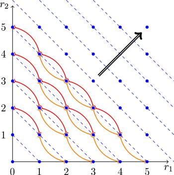
Figure 1. Algorithm for tensor reduction of sunset topology, where every point represents a particular tensor configuration (r1, r2). After using the |
4.4. Rank level four
There are five rank configurations and the expansion (2.13 ) is
$\begin{eqnarray}\begin{array}{l}{{\bf{C}}}^{(\mathrm{4,0})}={\vec{\alpha }}_{0,0,0}^{(4,0)}{s}_{00}^{2}+{\vec{\alpha }}_{2,0,0}^{(4,0)}{s}_{00}{s}_{01}^{2}+{\vec{\alpha }}_{4,0,0}^{(4,0)}{s}_{01}^{4},\\ {{\bf{C}}}_{1,1,1}^{(3,1)}={\vec{\alpha }}_{0,0,1}^{(3,1)}{s}_{00}{s}_{00^{\prime} }+{\vec{\alpha }}_{1,1,0}^{(3,1)}{s}_{00}{s}_{01}{s}_{0^{\prime} 1}+{\vec{\alpha }}_{2,0,1}^{(3,1)}{s}_{01}^{2}{s}_{00^{\prime} }+{\vec{\alpha }}_{3,1,0}^{(3,1)}{s}_{01}^{3}{s}_{0^{\prime} 1}\\ {{\bf{C}}}^{(\mathrm{2,2})}={\vec{\alpha }}_{0,0,2}^{(2,2)}{s}_{00^{\prime} }^{2}+{\vec{\alpha }}_{0,2,0}^{(2,2)}{s}_{00}{s}_{0^{\prime} 1}^{2}+{\vec{\alpha }}_{1,1,1}^{(2,2)}{s}_{01}{s}_{00^{\prime} }{s}_{0^{\prime} 1}+{\vec{\alpha }}_{2,2,0}^{(2,2)}{s}_{01}^{2}{s}_{0^{\prime} 1}^{2}+{\vec{\alpha }}_{0,0,0}^{(2,2)}{s}_{00}{s}_{0^{\prime} 0^{\prime} }+{\vec{\alpha }}_{2,0,0}^{(2,2)}{s}_{01}^{2}{s}_{0^{\prime} 0^{\prime} },\\ {{\bf{C}}}^{(\mathrm{1,3})}={\vec{\alpha }}_{0,0,1}^{(1,3)}{s}_{00^{\prime} }{s}_{0^{\prime} 0^{\prime} }+{\vec{\alpha }}_{0,2,1}^{(1,3)}{s}_{00^{\prime} }{s}_{0^{\prime} 1}^{2}+{\vec{\alpha }}_{1,1,0}^{(1,3)}{s}_{01}{s}_{0^{\prime} 1}{s}_{0^{\prime} 0^{\prime} }+{\vec{\alpha }}_{1,3,0}^{(1,3)}{s}_{01}{s}_{0^{\prime} 1}^{3},\\ {{\bf{C}}}^{(\mathrm{0,4})}={\vec{\alpha }}_{0,0,0}^{(0,4)}{s}_{0^{\prime} 0^{\prime} }^{2}+{\vec{\alpha }}_{0,2,0}^{(0,4)}{s}_{0^{\prime} 1}^{2}{s}_{0^{\prime} 0^{\prime} }+{\vec{\alpha }}_{0,4,0}^{(0,4)}{s}_{0^{\prime} 1}^{4}.\end{array}\end{eqnarray}$
One can get 34 linear equations from ${ \mathcal T }$ -type and ${ \mathcal D }$ -type relations for these 20 expansion coefficients. We can pick 20 independent equations among them. There are 18 ${ \mathcal T }$ -type equations${ \mathcal D }$ -type equations, we have
Picking 20 independent equations, we can solve all expansion coefficients of rank level four. Since its expression is long, we present them in an attached Mathematica file. All coefficients have been checked with the analytic output of FIRE [38, 39, 41].
$\begin{eqnarray}\begin{array}{l}\left\{4D{\vec{\alpha }}_{0,0,0}^{(0,4)}+8{\vec{\alpha }}_{0,0,0}^{(0,4)}+2{s}_{11}{\vec{\alpha }}_{0,2,0}^{(0,4)},2D{\vec{\alpha }}_{0,2,0}^{(0,4)}+8{\vec{\alpha }}_{0,2,0}^{(0,4)}+12{s}_{11}{\vec{\alpha }}_{0,4,0}^{(0,4)},2D{\vec{\alpha }}_{0,0,1}^{(1,3)}+4{\vec{\alpha }}_{0,0,1}^{(1,3)}+2{s}_{11}{\vec{\alpha }}_{0,2,1}^{(1,3)},\right.\\ 2D{\vec{\alpha }}_{1,1,0}^{(1,3)}+4{\vec{\alpha }}_{0,2,1}^{(1,3)}+4{\vec{\alpha }}_{1,1,0}^{(1,3)}+6{s}_{11}{\vec{\alpha }}_{1,3,0}^{(1,3)},D{\vec{\alpha }}_{0,0,1}^{(1,3)}+2{\vec{\alpha }}_{0,0,1}^{(1,3)}+{s}_{11}{\vec{\alpha }}_{1,1,0}^{(1,3)},\\ D{\vec{\alpha }}_{0,2,1}^{(1,3)}+2{\vec{\alpha }}_{0,2,1}^{(1,3)}+2{\vec{\alpha }}_{1,1,0}^{(1,3)}+3{s}_{11}{\vec{\alpha }}_{1,3,0}^{(1,3)},2D{\vec{\alpha }}_{0,0,0}^{(2,2)}+2{\vec{\alpha }}_{0,0,2}^{(2,2)}+2{s}_{11}{\vec{\alpha }}_{2,0,0}^{(2,2)},\\ 2D{\vec{\alpha }}_{0,2,0}^{(2,2)}+2{\vec{\alpha }}_{1,1,1}^{(2,2)}+2{s}_{11}{\vec{\alpha }}_{2,2,0}^{(2,2)},2D{\vec{\alpha }}_{0,0,0}^{(2,2)}+2{\vec{\alpha }}_{0,0,2}^{(2,2)}+2{s}_{11}{\vec{\alpha }}_{0,2,0}^{(2,2)},2D{\vec{\alpha }}_{2,0,0}^{(2,2)}+2{\vec{\alpha }}_{1,1,1}^{(2,2)}+2{s}_{11}{\vec{\alpha }}_{2,2,0}^{(2,2)},\\ 2D{\vec{\alpha }}_{0,0,2}^{(2,2)}+4{\vec{\alpha }}_{0,0,0}^{(2,2)}+2{\vec{\alpha }}_{0,0,2}^{(2,2)}+{s}_{11}{\vec{\alpha }}_{1,1,1}^{(2,2)},D{\vec{\alpha }}_{1,1,1}^{(2,2)}+4{\vec{\alpha }}_{0,2,0}^{(2,2)}+2{\vec{\alpha }}_{1,1,1}^{(2,2)}+4{\vec{\alpha }}_{2,0,0}^{(2,2)}+4{s}_{11}{\vec{\alpha }}_{2,2,0}^{(2,2)},\\ 2D{\vec{\alpha }}_{0,0,1}^{(3,1)}+4{\vec{\alpha }}_{0,0,1}^{(3,1)}+2{s}_{11}{\vec{\alpha }}_{2,0,1}^{(3,1)},2D{\vec{\alpha }}_{1,1,0}^{(3,1)}+4{\vec{\alpha }}_{1,1,0}^{(3,1)}+4{\vec{\alpha }}_{2,0,1}^{(3,1)}+6{s}_{11}{\vec{\alpha }}_{3,1,0}^{(3,1)},\\ D{\vec{\alpha }}_{0,0,1}^{(3,1)}+2{\vec{\alpha }}_{0,0,1}^{(3,1)}+{s}_{11}{\vec{\alpha }}_{1,1,0}^{(3,1)},D{\vec{\alpha }}_{2,0,1}^{(3,1)}+2{\vec{\alpha }}_{1,1,0}^{(3,1)}+2{\vec{\alpha }}_{2,0,1}^{(3,1)}+3{s}_{11}{\vec{\alpha }}_{3,1,0}^{(3,1)},4D{\vec{\alpha }}_{0,0,0}^{(4,0)}+8{\vec{\alpha }}_{0,0,0}^{(4,0)}+2{s}_{11}{\vec{\alpha }}_{2,0,0}^{(4,0)},\\ \left.2D{\vec{\alpha }}_{2,0,0}^{(4,0)}+8{\vec{\alpha }}_{2,0,0}^{(4,0)}+12{s}_{11}{\vec{\alpha }}_{4,0,0}^{(4,0)}\right\}=\mathrm{Known}\ \mathrm{Terms}.\end{array}\end{eqnarray}$
For 16 | • | reducing ℓ1 first $\begin{eqnarray}\begin{array}{l}\left\{\tfrac{1}{3}(D-2){\vec{\alpha }}_{0,0,0}^{(0,4)}+\tfrac{2}{3}(D-2){\vec{\alpha }}_{0,0,1}^{(1,3)}+\tfrac{1}{6}(D-2){s}_{11}{\vec{\alpha }}_{0,2,0}^{(0,4)}+\tfrac{2}{3}(D-2){s}_{11}{\vec{\alpha }}_{0,2,1}^{(1,3)},\right.\\ \tfrac{1}{6}(D-2){\vec{\alpha }}_{0,0,0}^{(0,4)}+\tfrac{1}{3}(D-2){\vec{\alpha }}_{0,0,1}^{(1,3)}+\tfrac{1}{12}(D-2){s}_{11}{\vec{\alpha }}_{0,2,0}^{(0,4)}+\tfrac{1}{3}(D-2){s}_{11}{\vec{\alpha }}_{1,1,0}^{(1,3)},\\ \tfrac{1}{4}(D-2){\vec{\alpha }}_{0,2,0}^{(0,4)}+\tfrac{1}{3}(D-2){\vec{\alpha }}_{0,2,1}^{(1,3)}+\tfrac{2}{3}(D-2){\vec{\alpha }}_{1,1,0}^{(1,3)}+\tfrac{1}{2}(D-2){s}_{11}{\vec{\alpha }}_{0,4,0}^{(0,4)}+(D-2){s}_{11}{\vec{\alpha }}_{1,3,0}^{(1,3)},\\ \tfrac{1}{6}D{\vec{\alpha }}_{0,0,1}^{(1,3)}+(D-1){\vec{\alpha }}_{0,0,0}^{(2,2)}+\tfrac{1}{6}{{Ds}}_{11}{\vec{\alpha }}_{0,2,1}^{(1,3)}+(D-1){s}_{11}{\vec{\alpha }}_{0,2,0}^{(2,2)},\\ \tfrac{1}{3}D{\vec{\alpha }}_{0,0,1}^{(1,3)}+(D-1){\vec{\alpha }}_{0,0,2}^{(2,2)}+\tfrac{1}{6}{{Ds}}_{11}{\vec{\alpha }}_{0,2,1}^{(1,3)}+\tfrac{1}{6}{{Ds}}_{11}{\vec{\alpha }}_{1,1,0}^{(1,3)}+\tfrac{1}{2}(D-1){s}_{11}{\vec{\alpha }}_{1,1,1}^{(2,2)},\\ \tfrac{1}{6}D{\vec{\alpha }}_{0,2,1}^{(1,3)}+\tfrac{1}{3}D{\vec{\alpha }}_{1,1,0}^{(1,3)}+\tfrac{1}{2}(D-1){\vec{\alpha }}_{1,1,1}^{(2,2)}+(D-1){\vec{\alpha }}_{2,0,0}^{(2,2)}+\tfrac{1}{2}{{Ds}}_{11}{\vec{\alpha }}_{1,3,0}^{(1,3)}+(D-1){s}_{11}{\vec{\alpha }}_{2,2,0}^{(2,2)},\\ \tfrac{1}{2}(D+2){\vec{\alpha }}_{0,0,0}^{(2,2)}+\tfrac{1}{2}(D+2){\vec{\alpha }}_{0,0,2}^{(2,2)}+D{\vec{\alpha }}_{0,0,1}^{(3,1)}+\tfrac{1}{2}(D+2){s}_{11}{\vec{\alpha }}_{0,2,0}^{(2,2)}+\tfrac{1}{4}(D+2){s}_{11}{\vec{\alpha }}_{1,1,1}^{(2,2)}+{{Ds}}_{11}{\vec{\alpha }}_{1,1,0}^{(3,1)},\\ \left.\tfrac{1}{4}(D+2){\vec{\alpha }}_{1,1,1}^{(2,2)}+\tfrac{1}{2}(D+2){\vec{\alpha }}_{2,0,0}^{(2,2)}+D{\vec{\alpha }}_{2,0,1}^{(3,1)}+\tfrac{1}{2}(D+2){s}_{11}{\vec{\alpha }}_{2,2,0}^{(2,2)}+{{Ds}}_{11}{\vec{\alpha }}_{3,1,0}^{(3,1)}\right\}=\mathrm{Known}\ \mathrm{Terms}.\end{array}\end{eqnarray}$ |
| • | reducing ℓ2 first $\begin{eqnarray}\begin{array}{l}\left\{D{\vec{\alpha }}_{0,0,1}^{(1,3)}+\tfrac{1}{2}(D+2){\vec{\alpha }}_{0,0,0}^{(2,2)}+\tfrac{1}{2}(D+2){\vec{\alpha }}_{0,0,2}^{(2,2)}+{{Ds}}_{11}{\vec{\alpha }}_{1,1,0}^{(1,3)}+\tfrac{1}{4}(D+2){s}_{11}{\vec{\alpha }}_{1,1,1}^{(2,2)}+\tfrac{1}{2}(D+2){s}_{11}{\vec{\alpha }}_{2,0,0}^{(2,2)},\right.\\ D{\vec{\alpha }}_{0,2,1}^{(1,3)}+\tfrac{1}{2}(D+2){\vec{\alpha }}_{0,2,0}^{(2,2)}+\tfrac{1}{4}(D+2){\vec{\alpha }}_{1,1,1}^{(2,2)}+{{Ds}}_{11}{\vec{\alpha }}_{1,3,0}^{(1,3)}+\tfrac{1}{2}(D+2){s}_{11}{\vec{\alpha }}_{2,2,0}^{(2,2)},\\ (D-1){\vec{\alpha }}_{0,0,2}^{(2,2)}+\tfrac{1}{3}D{\vec{\alpha }}_{0,0,1}^{(3,1)}+\tfrac{1}{2}(D-1){s}_{11}{\vec{\alpha }}_{1,1,1}^{(2,2)}+\tfrac{1}{6}{{Ds}}_{11}{\vec{\alpha }}_{1,1,0}^{(3,1)}+\tfrac{1}{6}{{Ds}}_{11}{\vec{\alpha }}_{2,0,1}^{(3,1)},\\ (D-1){\vec{\alpha }}_{0,0,0}^{(2,2)}+\tfrac{1}{6}D{\vec{\alpha }}_{0,0,1}^{(3,1)}+(D-1){s}_{11}{\vec{\alpha }}_{2,0,0}^{(2,2)}+\tfrac{1}{6}{{Ds}}_{11}{\vec{\alpha }}_{2,0,1}^{(3,1)},\\ (D-1){\vec{\alpha }}_{0,2,0}^{(2,2)}+\tfrac{1}{2}(D-1){\vec{\alpha }}_{1,1,1}^{(2,2)}+\tfrac{1}{3}D{\vec{\alpha }}_{1,1,0}^{(3,1)}+\tfrac{1}{6}D{\vec{\alpha }}_{2,0,1}^{(3,1)}+(D-1){s}_{11}{\vec{\alpha }}_{2,2,0}^{(2,2)}+\tfrac{1}{2}{{Ds}}_{11}{\vec{\alpha }}_{3,1,0}^{(3,1)},\\ \tfrac{1}{3}(D-2){\vec{\alpha }}_{0,0,1}^{(3,1)}+\tfrac{1}{6}(D-2){\vec{\alpha }}_{0,0,0}^{(4,0)}+\tfrac{1}{3}(D-2){s}_{11}{\vec{\alpha }}_{1,1,0}^{(3,1)}+\tfrac{1}{12}(D-2){s}_{11}{\vec{\alpha }}_{2,0,0}^{(4,0)},\\ \tfrac{2}{3}(D-2){\vec{\alpha }}_{0,0,1}^{(3,1)}+\tfrac{1}{3}(D-2){\vec{\alpha }}_{0,0,0}^{(4,0)}+\tfrac{2}{3}(D-2){s}_{11}{\vec{\alpha }}_{2,0,1}^{(3,1)}+\tfrac{1}{6}(D-2){s}_{11}{\vec{\alpha }}_{2,0,0}^{(4,0)},\\ \left.\tfrac{2}{3}(D-2){\vec{\alpha }}_{1,1,0}^{(3,1)}+\tfrac{1}{3}(D-2){\vec{\alpha }}_{2,0,1}^{(3,1)}+\tfrac{1}{4}(D-2){\vec{\alpha }}_{2,0,0}^{(4,0)}+(D-2){s}_{11}{\vec{\alpha }}_{3,1,0}^{(3,1)}+\tfrac{1}{2}(D-2){s}_{11}{\vec{\alpha }}_{4,0,0}^{(4,0)}\right\}\\ =\ \mathrm{Known}\ \mathrm{Terms}.\end{array}\end{eqnarray}$ |
Before ending this section, let us summarize the algorithm to reduce tensor integrals of sunset topology to the master basis. The number of expansion coefficients for a particular rank level r is given by${N}_{c}(m)=\lfloor \tfrac{m}{2}\rfloor +1$ is the number of expansion coefficients for a one-loop rank-m tensor bubble. The recursion procedure can be nicely represented in figure 1.
$\begin{eqnarray}\begin{array}{l}{N}_{\vec{a}}[r]=\sum _{{r}_{1}+{r}_{2}=r}\sum _{j=0}^{\min \{{r}_{1},{r}_{2}\}}{N}_{c}({r}_{1}-j){N}_{c}({r}_{2}-j)\end{array}\end{eqnarray}$
where 5. Conclusion and outlook
In this paper, we have taken the first step in generalizing our improved PV-reduction method with auxiliary vector R to two-loop integrals, i.e., we have carried out the tensor reduction for the simplest sunset topology. For two-loop integrals, the ${ \mathcal T }$ -type relations can be established straightforwardly, while the ${ \mathcal D }$ -type relations are rather nontrivial. We need to consider the reduction of its sub-one-loop integrals first. Combining the two types of relations, one can solve all expansion coefficients with the proper choice of master basis.
One of our motivations for the paper is to find an alternative method for higher loop tensor reduction other than the IBP method. Comparing these two methods, one can find some similarities. All IBP relations are generated by following six primary relations $\int \tfrac{\partial }{\partial {{\ell }}_{i}}\cdot {K}_{j}$ with i = 1, 2 and Kj = (ℓ1, ℓ2, K). Similarly, in our algorithm, there are also six operators ${\widetilde{K}}_{j}\cdot \tfrac{\partial }{{\dot{R}}_{i}}$ with i = 1, 2 and ${\widetilde{K}}_{j}=({R}_{1},{R}_{2},K)$ . The one-to-one mapping between these two types of manipulations seems to hint at a deep connection between these two methods although we are not clear at this moment. As pointed out in the paper, in our algorithm we have avoided the appearance of higher power propagators, thus the number of equations one needs to solve is much fewer than that using the standard IBP method. However, in [52] an idea has been suggested to avoid the higher power of propagators in the IBP method. It will be interesting to see if such an idea can be used in our algorithm.
There are several interesting questions coming from this work. The first one is that, in section 3 , we have discussed the choice of master integrals to be evaluating the ISP. We hope that for arbitrary two-loop or higher loop integrals with general masses and momenta K, one can determine the master basis from this perspective.
The second question is the following. As emphasized several times, the nontrivial ${ \mathcal D }$ -type relations depend crucially on the reduction relation (3.17 ) of one-loop integrals. We have tested the reduction of triangles and found similar reduction relation also holds for several examples. We find such a reduction relation holds for general one-loop integrals with the proof being presented in [50].
The third problem is obvious. In this paper, we focus on the sunset topology. There are other topologies for two-loop integrals. One needs to check if the algorithm present in this paper can be generalized to these cases. With results from higher topologies, we can reduce sunset with propagators having higher power using the idea given in [49]. We hope to give a positive answer to these interesting questions in our future work.