


1. Introduction
Although it has been over two decades since the Bosenova experiment [1], an accurate theoretical description of the collapse dynamics of Bose–Einstein condensates (BECs) [2–4] subjected to a sudden change of interatomic interaction to become sufficiently attractive is still elusive. Whereas the theoretical simulations based on the time-dependent Gross–Pitaevskii equation (GPE) with a three-body loss term provide an excellent qualitative understanding of many aspects of the experiments [5–13], satisfactory quantitative agreement with the experimental observations has not been achieved. These failures may be ascribed to the neglect of high order effects such as excitation or fluctuations driven by the dynamics of the condensates.
In [14], Calzetta and Hu considered the impact of the fluctuations on the evolution of the condensates. Similarly, Yurovsky introduced the fluctuations by linearizing the exact quantum equations of motion for the field operators and attributed loss from the condensate to the growth of the fluctuation [15]. Calzetta also showed that the growth of fluctuations led to a shorter collapse time for a collapsing condensate [16]. It should be noted that fluctuations were not self-consistently included in the above studies. In an improved treatment, Milstein et al studied the collapse dynamics of a condensate using the Hartree–Fock–Bogoliubov (HFB) theory [17]; however, the three-body loss was completely ignored in this work. In similar simulations employing the HFB theory, the three-body loss was only taken into account in the evolution equation for the condensate [18–20]. Thus the fluctuations are essentially treated as a pure state. The collapses were also simulated using the truncated Wigner method with random noise and a background thermal component in the initial state [19, 21].
In the present work, we revisit the collapse dynamics of a trapped single-component condensate by using the Gaussian state theory (GST) for mixed states [22]. By adopting a Gaussian formed density matrix, we derive, from the master equation, the dynamical equations for condensate wave function, the normal and anomalous fluctuations in the presence of three-body loss. These equations combined with the initial state obtained from the Gaussian state calculations provide a self-consistent description for the coherent condensate, excitation, and quantum depletion. Our theory is equivalent to the HFB theory except that the three-body loss is now properly treated in the dynamic equations for both condensate and fluctuations. To make the numerical simulations tractable, we assume a spherical symmetry for the system regardless of the realistic experimental setups. As a result, the main purpose of this work is not to quantitatively reproduce the experimental measurements. Instead, we focus on the new physics originating from the beyond mean-field effects. In fact, we identify the deferred collapses which are assisted by the fluctuations. As a result, the critical interaction strength for the weak collapse is smaller than that predicted by GPE. In addition, we show that due to the atom decay and strong interaction during collapse, a large fraction of atoms are transferred into the fluctuations in collapse such that the collapsed gas significantly deviated from a pure state. It is therefore inappropriate to treat the collapsed atom as a pure coherent state, although the calculation for atom number of the collapsed condensate does not appear to have much difference.
This paper is organized as follows. In section 2 , we introduce our model and derive the dynamic equations for the condensate, the normal, and the anomalous Green functions based on the master equation. In section 3 , we unveil the structure of the fluctuations by analyzing the normal and anomalous Green functions. Our simulation results are presented in section 4 . In particular, we show that there exists a new type of collapse assisted by the fluctuations. Finally, we conclude in section 5 .
2. Formulation
We consider a condensate of N trapped Bose atoms interacting via s-wave collision. In the second-quantized form, the Hamiltonian of the system reads$\hat{\psi }({\boldsymbol{r}})$ is the field operator, ${\hat{h}}_{0}=-{{\hslash }}^{2}{{\rm{\nabla }}}^{2}/(2m)+m{\omega }_{\mathrm{ho}}^{2}{r}^{2}/2$ is the single-particle Hamiltonian with m being the mass of the atom and ωho the frequency of the isotropic harmonic trap, g2 = 4πℏ2as/(2m) is the two-body interaction strength with as being the s-wave scattering length.
$\begin{eqnarray}H=\int {\rm{d}}{\boldsymbol{r}}{\hat{\psi }}^{\dagger }({\boldsymbol{r}}){\hat{h}}_{0}\hat{\psi }({\boldsymbol{r}})+\displaystyle \frac{{g}_{2}}{2}\int {\rm{d}}{\boldsymbol{r}}{\hat{\psi }}^{\dagger }({\boldsymbol{r}}){\hat{\psi }}^{\dagger }({\boldsymbol{r}})\hat{\psi }({\boldsymbol{r}})\hat{\psi }({\boldsymbol{r}}),\end{eqnarray}$
where In the presence of atom loss, the system is described by the density matrix ρ satisfying the Lindblad equation${\hat{\psi }}^{3}({\boldsymbol{r}})$ is the jump operator describing the three-body loss with γ3 being the loss coefficient. Within the framework of GST, the system is described by three order parameters: the coherent state wave function $\phi ({\boldsymbol{r}})=\mathrm{Tr}\left[\rho \hat{\psi }({\boldsymbol{r}})\right]$ , the Green function $G({\boldsymbol{r}},{\boldsymbol{r}}^{\prime} )=\mathrm{Tr}\left[\rho \delta {\hat{\psi }}^{\dagger }({{\boldsymbol{r}}}^{{\prime} })\delta \hat{\psi }({\boldsymbol{r}})\right]$ , and the anomalous Green function $F({\boldsymbol{r}},{\boldsymbol{r}}^{\prime} )=\mathrm{Tr}\left[\rho \delta \hat{\psi }({{\boldsymbol{r}}}^{{\prime} })\delta \hat{\psi }({\boldsymbol{r}})\right]$ , where $\delta \hat{\psi }({\boldsymbol{r}})=\hat{\psi }({\boldsymbol{r}})-\phi ({\boldsymbol{r}})$ is the fluctuation field. Apparently, G and F characterize the fluctuation of the system. To find the dynamical equation of φ, we multiply equation (2 ) by $\hat{\psi }$ and then take the trace, which leads to$G({\boldsymbol{r}},{\boldsymbol{r}}^{\prime} )$ and $F({\boldsymbol{r}},{\boldsymbol{r}}^{\prime} )$ as3 ) reduces to the GPE with the three-body loss being included [13], i.e.,4 ) and (5 ) are exact HFB equations for the normal and anomalous Green functions if the three-body loss is neglected.
$\begin{eqnarray}\begin{array}{cc}{\rm{i}}\hslash {{\rm{\partial }}}_{t}\rho = & [H,\rho ]-{\rm{i}}\hslash \frac{{\gamma }_{3}}{3!}\left\{\int {\rm{d}}{\boldsymbol{r}}{\left[{\psi }^{\dagger }({\boldsymbol{r}})\right]}^{3}\psi ({\boldsymbol{r}}{)}^{3},\rho \right\}\\ & +{\rm{i}}\hslash \frac{{\gamma }_{3}}{3}\int {\rm{d}}{\boldsymbol{r}}\psi ({\boldsymbol{r}}{)}^{3}\rho {\left[{\psi }^{\dagger }({\boldsymbol{r}})\right]}^{3},\end{array}\end{eqnarray}$
where { · , · } represents the anticommutator, $\begin{eqnarray}\begin{array}{l}{\rm{i}}{\partial }_{t}\phi ({\boldsymbol{r}})={\hat{h}}_{0}\phi ({\boldsymbol{r}})+{g}_{2}\left[| \phi ({\boldsymbol{r}}){| }^{2}+2G({\boldsymbol{r}},{\boldsymbol{r}})\right]\phi ({\boldsymbol{r}})\\ +{g}_{2}F({\boldsymbol{r}},{\boldsymbol{r}}){\phi }^{* }({\boldsymbol{r}})-{\rm{i}}{\hslash }\displaystyle \frac{{\gamma }_{3}}{2}\left[| \phi ({\boldsymbol{r}}){| }^{4}\phi ({\boldsymbol{r}})\right.\\ +6G({\boldsymbol{r}},{\boldsymbol{r}})| \phi ({\boldsymbol{r}}){| }^{2}\phi ({\boldsymbol{r}})\\ +3F({\boldsymbol{r}},{\boldsymbol{r}})| \phi ({\boldsymbol{r}}){| }^{2}{\phi }^{* }({\boldsymbol{r}})+{F}^{* }({\boldsymbol{r}},{\boldsymbol{r}}){\phi }^{3}({\boldsymbol{r}})\\ +6{G}^{2}({\boldsymbol{r}},{\boldsymbol{r}})\phi ({\boldsymbol{r}})+3| F({\boldsymbol{r}},{\boldsymbol{r}}){| }^{2}\phi ({\boldsymbol{r}})\\ \left.+6G({\boldsymbol{r}},{\boldsymbol{r}})F({\boldsymbol{r}},{\boldsymbol{r}}){\phi }^{* }({\boldsymbol{r}})\right].\end{array}\end{eqnarray}$
Following a similar procedure, we obtain the dynamical equations for $\begin{eqnarray}\begin{array}{l}{\rm{i}}{\partial }_{t}G({\boldsymbol{r}},{\boldsymbol{r}}^{\prime} )=\displaystyle \int {\rm{d}}{\boldsymbol{r}}^{\prime\prime} \left\{{ \mathcal E }({\boldsymbol{r}},{\boldsymbol{r}}^{\prime\prime} )G({\boldsymbol{r}}^{\prime\prime} ,{\boldsymbol{r}}^{\prime} )\right.\\ +{\rm{\Delta }}({\boldsymbol{r}},{\boldsymbol{r}}^{\prime\prime} ){F}^{* }({\boldsymbol{r}}^{\prime\prime} ,{\boldsymbol{r}}^{\prime} )-\left[{ \mathcal E }({\boldsymbol{r}}^{\prime} ,{\boldsymbol{r}}^{\prime\prime} )G({\boldsymbol{r}}^{\prime\prime} ,{\boldsymbol{r}})\right.\\ \left.{\left.+{\rm{\Delta }}({\boldsymbol{r}}^{\prime} ,{\boldsymbol{r}}^{\prime\prime} ){F}^{* }({\boldsymbol{r}}^{\prime\prime} ,{\boldsymbol{r}})\right]}^{\dagger }\right\},\end{array}\end{eqnarray}$
$\begin{eqnarray}\begin{array}{l}{\rm{i}}{\partial }_{t}F({\boldsymbol{r}},{\boldsymbol{r}}^{\prime} )={\rm{\Delta }}({\boldsymbol{r}},{\boldsymbol{r}}^{\prime} )\delta ({\boldsymbol{r}}-{\boldsymbol{r}}^{\prime} )\\ +\displaystyle \int {\rm{d}}{\boldsymbol{r}}^{\prime\prime} \left\{{ \mathcal E }({\boldsymbol{r}},{\boldsymbol{r}}^{\prime\prime} )F({\boldsymbol{r}}^{\prime\prime} ,{\boldsymbol{r}}^{\prime} )+G({\boldsymbol{r}},{\boldsymbol{r}}^{\prime\prime} ){\rm{\Delta }}({\boldsymbol{r}}^{\prime\prime} ,{\boldsymbol{r}}^{\prime} )\right.\\ \left.+{\left[{ \mathcal E }({\boldsymbol{r}}^{\prime} ,{\boldsymbol{r}}^{\prime\prime} )F({\boldsymbol{r}}^{\prime\prime} ,{\boldsymbol{r}})+G({\boldsymbol{r}}^{\prime} ,{\boldsymbol{r}}^{\prime\prime} ){\rm{\Delta }}({\boldsymbol{r}}^{\prime\prime} ,{\boldsymbol{r}})\right]}^{{\rm{T}}}\right\},\end{array}\end{eqnarray}$
where $\begin{eqnarray}\begin{array}{l}{ \mathcal E }({\boldsymbol{r}},{{\boldsymbol{r}}}^{{\prime} })={\hat{h}}_{0}+2{g}_{2}\left[| \phi ({\boldsymbol{r}}){| }^{2}+G({\boldsymbol{r}},{\boldsymbol{r}})\right]\delta ({\boldsymbol{r}}-{{\boldsymbol{r}}}^{{\prime} })\\ -{\rm{i}}{\hslash }\displaystyle \frac{3{\gamma }_{3}}{2}\left[| \phi ({\boldsymbol{r}}){| }^{4}+4G({\boldsymbol{r}},{\boldsymbol{r}})| \phi ({\boldsymbol{r}}){| }^{2}+F({\boldsymbol{r}},{\boldsymbol{r}}){\phi }^{* 2}({\boldsymbol{r}})\right.\\ \left.+{F}^{* }({\boldsymbol{r}},{\boldsymbol{r}}){\phi }^{2}({\boldsymbol{r}})+2{G}^{2}({\boldsymbol{r}},{\boldsymbol{r}})+| F({\boldsymbol{r}},{\boldsymbol{r}}){| }^{2}\right]\delta ({\boldsymbol{r}}-{{\boldsymbol{r}}}^{{\prime} }),\end{array}\end{eqnarray}$
$\begin{eqnarray}\begin{array}{l}{\rm{\Delta }}({\boldsymbol{r}},{{\boldsymbol{r}}}^{{\prime} })={g}_{2}\left[{\phi }^{2}({\boldsymbol{r}})+F({\boldsymbol{r}},{\boldsymbol{r}})\right]\delta ({\boldsymbol{r}}-{{\boldsymbol{r}}}^{{\prime} })\\ -{\rm{i}}{\hslash }{\gamma }_{3}\left[| \phi ({\boldsymbol{r}}){| }^{2}{\phi }^{2}({\boldsymbol{r}})+3G({\boldsymbol{r}},{\boldsymbol{r}}){\phi }^{2}({\boldsymbol{r}})\right.\\ \left.+3F({\boldsymbol{r}},{\boldsymbol{r}})| \phi ({\boldsymbol{r}}){| }^{2}+3G({\boldsymbol{r}},{\boldsymbol{r}})F({\boldsymbol{r}},{\boldsymbol{r}})\right]\delta ({\boldsymbol{r}}-{{\boldsymbol{r}}}^{{\prime} }).\end{array}\end{eqnarray}$
It can be easily shown that when the quantum fluctuations G and F are ignorable, equation ( $\begin{eqnarray}{\rm{i}}{\hslash }{\partial }_{t}\phi ({\boldsymbol{r}})=\left[{\hat{h}}_{0}+{g}_{2}| \phi ({\boldsymbol{r}}){| }^{2}-{\rm{i}}{\hslash }\displaystyle \frac{{\gamma }_{3}}{2}| \phi ({\boldsymbol{r}}){| }^{4}\right]\phi ({\boldsymbol{r}}).\end{eqnarray}$
In addition, equations (Physical quantities can be conveniently expressed in terms of these order parameters. For example, the density of the gas is$E=\mathrm{Tr}(\rho H)={E}_{\mathrm{kin}}+{E}_{\mathrm{int}}$ , where
$\begin{eqnarray}n({\boldsymbol{r}})=\mathrm{Tr}[\rho {\hat{\psi }}^{\dagger }({\boldsymbol{r}})\hat{\psi }({\boldsymbol{r}})]=| \phi ({\boldsymbol{r}}){| }^{2}+G({\boldsymbol{r}},{\boldsymbol{r}}),\end{eqnarray}$
from which we deduce that the number of atoms in the coherent state and in the fluctuation are NC = ∫dr∣φ(r)∣2 and NF = ∫drG(r, r), respectively. Moreover, the total energy is $\begin{eqnarray}{E}_{\mathrm{kin}}=\int {\rm{d}}{\boldsymbol{r}}\left[{\phi }^{* }({\boldsymbol{r}}){h}_{0}({\boldsymbol{r}})\phi ({\boldsymbol{r}})+\mathop{\mathrm{lim}}\limits_{{\boldsymbol{r}}^{\prime} \to {\boldsymbol{r}}}{h}_{0}({\boldsymbol{r}}^{\prime} )G({\boldsymbol{r}}^{\prime} ,{\boldsymbol{r}})\right]\end{eqnarray}$
and $\begin{eqnarray}\begin{array}{l}{E}_{\mathrm{int}}=\displaystyle \frac{{g}_{2}}{2}\displaystyle \int {\rm{d}}{\boldsymbol{r}}\left\{| \phi ({\boldsymbol{r}}){| }^{4}+\left[{\phi }^{2}({\boldsymbol{r}}){F}^{* }({\boldsymbol{r}},{\boldsymbol{r}})+{\rm{c}}.{\rm{c}}.\right]\right.\\ \left.+4| \phi ({\boldsymbol{r}}){| }^{2}G({\boldsymbol{r}},{\boldsymbol{r}})+2G{\left({\boldsymbol{r}},{\boldsymbol{r}}\right)}^{2}+| F({\boldsymbol{r}},{\boldsymbol{r}}){| }^{2}\right\}\end{array}\end{eqnarray}$
are the kinetic and the interaction energies, respectively. Interestingly, in Eint, there are more terms contributed by the fluctuations through G and F, which suggests that the appearance of the fluctuations may amplify the interaction. This observation can be most easily confirmed by considering a macroscopic squeezed vacuum state, for which the attractive interaction is amplified by a factor of three [23].We shall study the collapse dynamics by numerically evolving equations (3 )–(5 ) simultaneously. To make our simulations numerically manageable, we utilize the spherical symmetry of the system by assuming that the order parameters are only functions of radii, i.e., φ(r), $G(r,r^{\prime} )$ , and $F(r,r^{\prime} )$ . To compare with the GPE theory, we shall also simulate the collapse dynamics using equation (8 ) by assuming that condensates are described by a pure coherent state.
3. Characterization of the fluctuations
Unlike in a pure Gaussian state where the fluctuations always represent the squeezing, fluctuations in a mixed Gaussian state also contain occupations of the quasiparticle states. To analyze the properties of the mixed Gaussian state, let us first write down the density matrix,$\hat{K}$ is a Hermitian operator and partition function $Z=\mathrm{Tr}(\rho )$ . In the Nambu basis $\delta \hat{{\rm{\Psi }}}({\boldsymbol{r}})={\left(\delta \hat{\psi }({\boldsymbol{r}}),\delta {\hat{\psi }}^{\dagger }({\boldsymbol{r}})\right)}^{{\rm{T}}}$ , $\hat{K}$ can be further expressed as${\rm{\Omega }}({\boldsymbol{r}},{\boldsymbol{r}}^{\prime} )=\left(\begin{array}{cc}A({\boldsymbol{r}},{\boldsymbol{r}}^{\prime} ) & B({\boldsymbol{r}},{\boldsymbol{r}}^{\prime} )\\ {\left[B({\boldsymbol{r}},{\boldsymbol{r}}^{\prime} )\right]}^{* } & {\left[A({\boldsymbol{r}},{\boldsymbol{r}}^{\prime} )\right]}^{* }\end{array}\right)$ subjected to the conditions${\boldsymbol{r}}^{\prime} $ being the indices for the matrix elements. As a result, condition (14 ) simply implies A† = A and BT = B.
$\begin{eqnarray}\rho =\displaystyle \frac{{{\rm{e}}}^{-\hat{K}}}{Z},\end{eqnarray}$
where $\begin{eqnarray}\hat{K}=\displaystyle \frac{1}{2}\int {\rm{d}}{\boldsymbol{r}}{\rm{d}}{\boldsymbol{r}}^{\prime} \delta {\hat{{\rm{\Psi }}}}^{\dagger }({\boldsymbol{r}}){\rm{\Omega }}({\boldsymbol{r}},{\boldsymbol{r}}^{\prime} )\delta \hat{{\rm{\Psi }}}({\boldsymbol{r}}^{\prime} ),\end{eqnarray}$
where $\begin{eqnarray}{\left[A({\boldsymbol{r}}^{\prime} ,{\boldsymbol{r}})\right]}^{* }=A({\boldsymbol{r}},{\boldsymbol{r}}^{\prime} )\,{\rm{and}}\,B({\boldsymbol{r}}^{\prime} ,{\boldsymbol{r}})=B({\boldsymbol{r}},{\boldsymbol{r}}^{\prime} ).\end{eqnarray}$
Alternatively, A and B can be regarded as matrices with r and To diagonalize $\hat{K}$ , we introduce the Bogoliubov transformation$\hat{\beta }=\left(\begin{array}{c}\hat{{\boldsymbol{b}}}\\ {\hat{{\boldsymbol{b}}}}^{\dagger }\end{array}\right)$ and $S({\boldsymbol{r}})=\left(\begin{array}{cc}{\boldsymbol{u}}({\boldsymbol{r}}) & {{\boldsymbol{v}}}^{* }({\boldsymbol{r}})\\ {\boldsymbol{v}}({\boldsymbol{r}}) & {{\boldsymbol{u}}}^{* }({\boldsymbol{r}})\end{array}\right)$ . More specifically, $\hat{{\boldsymbol{b}}}={\left({\hat{b}}_{1},{\hat{b}}_{2},\ldots \right)}^{{\rm{T}}}$ are Bogoliubov quasiparticles and u(r) = (u1(r), u2(r),…,ui(r), …) and v(r) = (v1(r), v2(r),…,vi(r), …) are the mode functions. Here we treat u and v as matrices with i and r being the (discrete) column and (continuous) row indices, respectively. Since Bogoliubov quasiparticles satisfy the bosonic commutation relations $[\hat{\beta },{\hat{\beta }}^{\dagger }]={\sigma }_{z}\otimes I$ , S must be a symplectic matrix, i.e.,${{\rm{\Sigma }}}_{z}({\boldsymbol{r}}-{\boldsymbol{r}}^{\prime} )={\sigma }_{z}\otimes \delta ({\boldsymbol{r}}-{\boldsymbol{r}}^{\prime} )$ . Writing out this equation explicitly, we obtain the completeness relation for the mode functions${{\rm{\Sigma }}}_{z}({\boldsymbol{r}}^{\prime} -{\boldsymbol{r}}^{\prime\prime} )S({\boldsymbol{r}}^{\prime\prime} )$ from left to both sides of the equation (16 ), we obtain the normalization conditions:
$\begin{eqnarray}\delta \hat{{\rm{\Psi }}}({\boldsymbol{r}})=S({\boldsymbol{r}})\hat{\beta },\end{eqnarray}$
where $\begin{eqnarray}S({\boldsymbol{r}})({\sigma }_{z}\otimes I){S}^{\dagger }({\boldsymbol{r}}^{\prime} )={{\rm{\Sigma }}}_{z}({\boldsymbol{r}}-{\boldsymbol{r}}^{\prime} ),\end{eqnarray}$
where I is an identity matrix and $\begin{eqnarray}\sum _{i}[{u}_{i}({\boldsymbol{r}}){u}_{i}^{* }({\boldsymbol{r}}^{\prime} )-{v}_{i}^{* }({\boldsymbol{r}}){v}_{i}({\boldsymbol{r}}^{\prime} )]=\delta ({\boldsymbol{r}}-{\boldsymbol{r}}^{\prime} ).\end{eqnarray}$
Moreover, multiplying $\begin{eqnarray}{S}^{\dagger }({\boldsymbol{r}}^{\prime} ){{\rm{\Sigma }}}_{z}({\boldsymbol{r}}^{\prime} -{\boldsymbol{r}}^{\prime\prime} )S({\boldsymbol{r}}^{\prime\prime} )={\sigma }_{z}\otimes I\end{eqnarray}$
or, equivalently, $\begin{eqnarray}\int {\rm{d}}{\boldsymbol{r}}[{u}_{i}({\boldsymbol{r}}){u}_{j}^{* }({\boldsymbol{r}})-{v}_{i}({\boldsymbol{r}}){v}_{j}^{* }({\boldsymbol{r}})]={\delta }_{{ij}}.\end{eqnarray}$
To proceed further, we assume that Ω is symplectically diagonalized by S as20 ) can be transformed into the familiar Bogoliubov equation15 ), i.e.,$G({\boldsymbol{r}},{\boldsymbol{r}}^{\prime} )={G}_{T}({\boldsymbol{r}},{\boldsymbol{r}}^{\prime} )+{G}_{Q}({\boldsymbol{r}},{\boldsymbol{r}}^{\prime} )$ and $F({\boldsymbol{r}},{\boldsymbol{r}}^{\prime} )={F}_{T}({\boldsymbol{r}},{\boldsymbol{r}}^{\prime} )+{F}_{Q}({\boldsymbol{r}},{\boldsymbol{r}}^{\prime} )$ . More specifically,${f}_{i}=\mathrm{tr}(\rho {\hat{b}}_{i}^{\dagger }{\hat{b}}_{i})=1/({{\rm{e}}}^{{d}_{i}}-1)$ is the average quasiparticle occupation number on the ith mode, in analogy to the thermal occupation number at finite temperature. Therefore, we may say that GT and FT characterize the thermal fluctuation even if the temperature of the system is zero. On the other hand,26 ) and (27 ), GQ and FQ can be simultaneously diagonalized by a set of orthonormal modes $\{{\bar{\phi }}_{S,\alpha }({\boldsymbol{r}})\}$ satisfying $\int {\rm{d}}{\boldsymbol{r}}{\bar{\phi }}_{S,\alpha }^{* }({\boldsymbol{r}}){\bar{\phi }}_{S,\alpha ^{\prime} }({\boldsymbol{r}})={\delta }_{\alpha \alpha ^{\prime} }$ . Therefore, similar to those in a pure Gaussian state, GQ and FQ characterize squeezing with NS,α being the occupation number in the αth squeezed mode ${\bar{\phi }}_{S,\alpha }$ . Then NS = ∑jNS,α is the total number of squeezed atoms. Without loss of generality, we assume that NS,α are sorted in descending order with respect to the index α. Thus ${\bar{\phi }}_{S,1}$ represents the squeezed mode with the highest occupation. Interestingly, the condensate is in a macroscopic squeezed state when ${\bar{\phi }}_{S,1}$ is macroscopically occupied [23–25]. And for a weakly attractive condensate, a condensate can even be in a pure single-mode squeezed state with ${\bar{\phi }}_{S,1}\simeq N$ . In this case, it can be clearly seen from equation (11 ) that the interaction energy is amplified by a factor of three [23].
$\begin{eqnarray}{S}^{\dagger }{\rm{\Omega }}S=D,\end{eqnarray}$
where D = I2 ⨂ d with I2 being a 2 × 2 identity matrix and d = diag{d1, d2,…,di, …} a diagonal matrix. Equation ( $\begin{eqnarray}{{\rm{\Sigma }}}_{z}{\rm{\Omega }}S=S{{\rm{\Sigma }}}_{z}D.\end{eqnarray}$
In the quasiparticle basis, the density matrix can be expressed as $\begin{eqnarray}\rho ={Z}^{-1}{{\rm{e}}}^{-{\hat{{\boldsymbol{b}}}}^{\dagger }{\boldsymbol{d}}\hat{{\boldsymbol{b}}}}={Z}^{-1}\exp \left(-\sum _{i}{d}_{i}{\hat{b}}_{i}^{\dagger }{\hat{b}}_{i}\right).\end{eqnarray}$
Making use of the explicit expression for the Bogoliubov transformation ( $\begin{eqnarray}\delta \hat{\psi }({\boldsymbol{r}})=\sum _{i}\left[{u}_{i}({\boldsymbol{r}}){\hat{b}}_{i}+{v}_{i}^{* }({\boldsymbol{r}}){\hat{b}}_{i}^{\dagger }\right],\end{eqnarray}$
the normal and anomalous Green functions can be decomposed into the forms $\begin{eqnarray}{G}_{T}({\boldsymbol{r}},{\boldsymbol{r}}^{\prime} )=\sum _{i}{f}_{i}\left({u}_{i}^{* }({\boldsymbol{r}}^{\prime} ){u}_{i}({\boldsymbol{r}})+{v}_{i}({\boldsymbol{r}}^{\prime} ){v}_{i}^{* }({\boldsymbol{r}})\right),\end{eqnarray}$
$\begin{eqnarray}{F}_{T}({\boldsymbol{r}},{\boldsymbol{r}}^{\prime} )=\sum _{i}{f}_{i}\left({v}_{i}^{* }({\boldsymbol{r}}^{\prime} ){u}_{i}({\boldsymbol{r}})+{u}_{i}({\boldsymbol{r}}^{\prime} ){v}_{i}^{* }({\boldsymbol{r}})\right),\end{eqnarray}$
where $\begin{eqnarray}\begin{array}{rcl}{G}_{Q}({\boldsymbol{r}},{\boldsymbol{r}}^{\prime} ) & = & \displaystyle \sum _{i}{v}_{i}({\boldsymbol{r}}^{\prime} ){v}_{i}^{* }({\boldsymbol{r}})\\ & = & \displaystyle \sum _{\alpha =1}^{\infty }{N}_{S,\alpha }{\bar{\phi }}_{S,\alpha }({\boldsymbol{r}}){\bar{\phi }}_{S,\alpha }^{* }({{\boldsymbol{r}}}^{{\prime} })\end{array}\end{eqnarray}$
and $\begin{eqnarray}\begin{array}{rcl}{F}_{Q}({\boldsymbol{r}},{\boldsymbol{r}}^{\prime} ) & = & \displaystyle \sum _{i}\displaystyle \frac{1}{2}\left({v}_{i}^{* }({\boldsymbol{r}}^{\prime} ){u}_{i}({\boldsymbol{r}})+{u}_{i}({\boldsymbol{r}}^{\prime} ){v}_{i}^{* }({\boldsymbol{r}})\right)\\ & = & \displaystyle \sum _{\alpha =1}^{\infty }\sqrt{{N}_{S,\alpha }({N}_{S,\alpha }+1)}{\bar{\phi }}_{S,\alpha }({\boldsymbol{r}}){\bar{\phi }}_{S,\alpha }({{\boldsymbol{r}}}^{{\prime} })\end{array}\end{eqnarray}$
are quantum fluctuation (or quantum depletion) which does not represent an actual occupation of the Bogoliubov excitation modes. Moreover, as shown in the second lines of equations (To distinguish different states, it is helpful to compute the second-order correlation function${g}_{\mathrm{coherent}}^{(2)}({\boldsymbol{r}},{\boldsymbol{r}})=1;$ (ii) For a thermal state, φ, GS, and FS are all zero. As a result, all vi(r)'s and, subsequently, F vanishes, which further yields ${g}_{\mathrm{thermal}}^{(2)}({\boldsymbol{r}},{\boldsymbol{r}})=2;$ (iii) For a pure squeezed state, we have NS,1 ≃ N. As a result, φ, GT, and FT vanish, which implies F(r, r) ≈ G(r, r) and, subsequently, ${g}_{\mathrm{squeeze}}^{(2)}({\boldsymbol{r}},{\boldsymbol{r}})\approx 3$ . Therefore, measuring g(2) should allow us to identify the state of a collapsed condensate.
$\begin{eqnarray}\begin{array}{rl}{g}^{(2)}({\boldsymbol{r}},{\boldsymbol{r}})\,= & \frac{{\rm{tr}}[\rho {\hat{\psi }}^{\dagger }({\boldsymbol{r}}){\hat{\psi }}^{\dagger }({\boldsymbol{r}})\hat{\psi }({\boldsymbol{r}})\hat{\psi }({\boldsymbol{r}})]}{{\rm{tr}}[\rho {\hat{\psi }}^{\dagger }({\boldsymbol{r}})\hat{\psi }({\boldsymbol{r}}){]}^{2}}\\ = & n({\boldsymbol{r}}{)}^{-2}\{| {\phi }^{(c)}({\boldsymbol{r}}){| }^{4}+2{G}^{2}({\boldsymbol{r}},{\boldsymbol{r}})+| F({\boldsymbol{r}},{\boldsymbol{r}}){| }^{2}\\ & +4G({\boldsymbol{r}},{\boldsymbol{r}})| {\phi }^{(c)}({\boldsymbol{r}}){| }^{2}+2{\rm{Re}}[{F}^{\ast }({\boldsymbol{r}},{\boldsymbol{r}}){\phi }^{(c)2}({\boldsymbol{r}})]\}.\end{array}\end{eqnarray}$
The following special cases are of particular importance. (i) For a pure coherent state, G and F vanish, which leads to Finally, we shall also use the entropy
$\begin{eqnarray}\begin{array}{rcl}{ \mathcal S }(\rho ) & = & -\mathrm{tr}(\rho \mathrm{ln}\rho )\\ & = & \sum _{i}\left[({f}_{i}+1)\mathrm{ln}({f}_{i}+1)-{f}_{i}\mathrm{ln}{f}_{i}\right]\end{array}\end{eqnarray}$
to measure the deviation of the collapsed condensate from a pure state.4. Results
To systematically explore the collapse dynamics, we first recall that the system is completely specified by the following parameters: atom number N, trap frequency ωho, scattering length as, and three-body loss coefficient γ3. Without loss of generality, the trap frequency is fixed at ωho = (2π)12.8 Hz which is the geometric average of the trap frequencies in three Cartesian directions of the experiment [2]. In all simulations, we prepare an initial pure state by numerically solving the imaginary-time equations of motion for a Gaussian state [23–25] under the initial atom number N(0) and scattering length as = ainit ( ≥ 0). We then quench the scattering length to as = afinal ( < 0) at t = 0. It should be noted that a trapped BEC with attractive interactions becomes unstable only when the dimensionless parameter (DIP)${a}_{\mathrm{ho}}=\sqrt{{\hslash }/(m{\omega }_{\mathrm{ho}})}$ is the harmonic oscillator length. For the chosen parameter, we have aho = 5.77 × 10⁴aB with aB being the Bohr radius. There exist many studies on the critical interaction strength of a trapped condensate [26–31]. The dynamics of the condensate are then simulated by numerically evolving equations (3 )–(5 ). We point out that, to minimize the impact of ainit on kcri, it is preferable to choose ainit = 0. However, in order to obtain an initial state with nonvanishing fluctuations, we normally adopt a very small ainit in our simulations.
$\begin{eqnarray}k=\displaystyle \frac{N| {a}_{{\rm{s}}}| }{{a}_{\mathrm{ho}}}\end{eqnarray}$
exceeds a critical value, say kcri, where As shall be shown, for the same set of N(0), ainit, and γ3, the GST and GPE approaches may lead to two distinct critical interaction strengths, say ${k}_{\mathrm{cri}}^{(\mathrm{gst})}$ and ${k}_{\mathrm{cri}}^{(\mathrm{gpe})}$ , which satisfy ${k}_{\mathrm{cri}}^{(\mathrm{gst})}\lt {k}_{\mathrm{cri}}^{(\mathrm{gpe})}$ . Consequently, based on the final interaction parameter kfinal, we categorize the collapses into (i) the direct collapse that happens when ${k}_{\mathrm{final}}\gt {k}_{\mathrm{cri}}^{(\mathrm{gpe})}$ and (ii) the deferred collapse which is stimulated by the fluctuations and occurs under the condition ${k}_{\mathrm{cri}}^{(\mathrm{gpe})}\gt {k}_{\mathrm{final}}\gt {k}_{\mathrm{cri}}^{(\mathrm{gst})}$ . In other words, a direct collapse also happens in the GPE simulations; while a deferred collapse only occurs when we simulate it using GST. In figure 1, we schematically show the parameter regimes for different types of collapses.
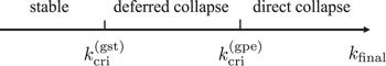
Figure 1. Schematic plot for the collapse types on the axis of DIP. |
4.1. Direct collapses
As an example of direct collapses, we perform simulations with the same set of control parameters as those used in the experiment [2], i.e., N(0) = 1.6 × 10⁴, ainit = 7aB, and afinal = −30aB. Correspondingly, the DIP kfinal = 8.32 is much larger than the critical interaction strength. Figures 2(a) and (b) plot the time dependence of the total atom number N and the peak condensate density npeak, respectively. Here the three-body loss coefficient is taken as γ3 = 3 × 10⁻²⁷cm6 s–1, a value obtained by fitting the atom number with experiment data [2] (dots in figure 2(a)). For comparison, we also present the results from the GPE simulation (dash-dotted lines). As can be seen, for atom number N(t), the results obtained via both approaches are in good agreement. However, for the peak density, a large discrepancy appears when t is roughly larger than 7 ms. In addition, our results are in qualitative agreement with the simulations presented in [5, 7].

Figure 2. (a) Time dependence of the total atom number computed via GST (solid line) and GPE (dash-dotted line). Filled circles (•) represent the experimental data [2]. The black dashed line shows the time dependence of NF (right y axis) obtained using GST. (b) Time dependence of the peak density computed via GST (solid line) and GPE (dash-dotted line). The black solid line shows the time dependence of the entropy per atom (right y axis). (c) Second-order correlation function g(2)(r, r) for t = 0 (dotted line), 3 (dashed line), 10 (dash-dotted line), and 30 ms (solid line). Other parameters are N(0) = 1.6 × 10⁴, ainit = 7aB, afinal = −30 aB, and γ3 = 3 × 10⁻²⁷cm6 s–1. |
For a typical direct collapse, after the scattering length is quenched, N roughly remains constant for some time and then experiences a sudden decay which signals a collapse of the condensate. The time of this collapse defines the collapse time tcoll. After tcoll, collapses occur intermittently such that N(t) decays stepwise. Associated with each collapse, there is a spike on the npeak–t curve, indicating that the condensate first implodes and then explodes. The underlying reason for the formation of the spikes was previously studied in [5, 7]. Specifically, during an implosion, the condensate shrinks and its peak density abruptly increases. Consequently, both the kinetic and the interaction energies increase. This process is also accompanied by the increase of the three-body loss which lowers npeak. When the atom loss rate becomes larger than the accumulation rate of the atoms, the peak density ceases to increase (see below for a detailed analysis). Now, because the kinetic and interaction energies are proportional to npeak and ${n}_{\mathrm{peak}}^{2}$ , respectively, the attractive interaction energy decreases faster than the kinetic energy. As a result, the attraction is insufficient to bound gas such that the condensate starts to explode and the peak density is quickly lowered.
This observation can be understood by a simple model described below. Within tcoll, the squeezed atoms in the condensate are negligible such that the condensate is solely described by φ(r). In addition, as the shape of the condensate is well maintained, φ can then be approximated by a Gaussian function
$\begin{eqnarray}\phi (r)={\left[\displaystyle \frac{N}{{\pi }^{3/2}\sigma {\left(t\right)}^{3}}\right]}^{1/2}{{\rm{e}}}^{-{r}^{2}/[2\sigma {\left(t\right)}^{2}]-{\rm{i}}{r}^{2}\beta (t)},\end{eqnarray}$
where σ is the width of the condensate and β(t) accounts for the dynamics due to the kinetic energy. It can be shown that σ satisfies the dynamics equation $\begin{eqnarray}m\displaystyle \frac{{{\rm{d}}}^{2}\sigma }{{{\rm{d}}{t}}^{2}}=-\displaystyle \frac{\partial {V}_{\mathrm{eff}}(\sigma )}{\partial \sigma },\end{eqnarray}$
where $\begin{eqnarray}{V}_{\mathrm{eff}}(\sigma )=\displaystyle \frac{1}{2}{\hslash }{\omega }_{\mathrm{ho}}\left(\displaystyle \frac{{\sigma }^{2}}{{a}_{\mathrm{ho}}^{2}}+\displaystyle \frac{{a}_{\mathrm{ho}}^{2}}{{\sigma }^{2}}-\displaystyle \frac{4{k}_{\mathrm{final}}}{3\sqrt{2\pi }}\displaystyle \frac{{a}_{\mathrm{ho}}^{3}}{{\sigma }^{3}}\right),\end{eqnarray}$
is the effective potential experienced by a particle with mass m. Clearly, Veff contains contributions from potential, kinetic, and interaction energies. Once σ(t) is obtained, β(t) can be evaluated according to $\begin{eqnarray}\beta (t)=\displaystyle \frac{m}{2{\hslash }\sigma }\displaystyle \frac{{\rm{d}}\sigma }{{\rm{d}}t}.\end{eqnarray}$
We now use this simple variational wave function to estimate the height of the first spikes on npeak–t curve. To this end, we first derive, from equation (8 ), a continuity equation${\boldsymbol{J}}=\tfrac{{\hslash }}{m}\mathrm{Im}({\phi }^{* }{\rm{\nabla }}\phi )$ . Making use of the ansatz (31 ), the continuity equation reduces to36 ), we obtain32 ) and (34 ) such that the condition (37 ) is satisfied. With the parameters used in figure 2, we find that tspike ≈ 4 ms and np(tspike) ≈ 1.0637 × 10²¹ m−3, which are in rough agreement with the full numerical simulation.
$\begin{eqnarray}{\partial }_{t}| \phi {| }^{2}=-{\rm{\nabla }}\cdot {\boldsymbol{J}}-{\hslash }{\gamma }_{3}| \phi {| }^{6},\end{eqnarray}$
where $\begin{eqnarray}\displaystyle \frac{{\rm{d}}}{{\rm{d}}t}{n}_{\mathrm{peak}}(t)=\displaystyle \frac{6{\hslash }\beta (t)}{m}{n}_{\mathrm{peak}}(t)-{\gamma }_{3}{n}_{\mathrm{peak}}^{3}(t),\end{eqnarray}$
where$\begin{eqnarray*}{n}_{\mathrm{peak}}(t)=\displaystyle \frac{{N}_{c}}{\pi \sqrt{\pi }\sigma {\left(t\right)}^{3}}\end{eqnarray*}$
is the peak density of the Gaussian density profile. The time for the first spike, i.e., tspike, can be determined using the condition that the peak density stops growing at t = tspike. Then from equation ( $\begin{eqnarray}\beta ({t}_{\mathrm{spike}})=\displaystyle \frac{m{\gamma }_{3}}{6{\hslash }}{n}_{\mathrm{peak}}^{2}({t}_{\mathrm{spike}}).\end{eqnarray}$
Now, to determine tspike, we numerically solve equations (Next, we compare the GST and the GPE descriptions of the collapse dynamics. To this end, we also plot, in figure 2(a), the number of the fluctuated atoms NF as a function of time t. Immediately after the collapse starts, NF quickly increases and then saturates at about 550 atoms after t ≈ 10 ms. In particular, NF/N can be as large as 30% at t = 30 ms, which suggests that the statistical property of the condensate might be dramatically modified. Moreover, as shown in figure 2(b), the entropy of the system monotonically increases and becomes nearly saturated at large t, indicating that the system significantly deviates from a pure state. To find more details, we present, in figure 2(c), the second-order correlation function g(2)(r, r) at various times. As expected, the second-order correlation function is unity for the initial state. Then for t = 3 ms, g(2)(r, r) begins to deviate from unity in the high-density region where the three-body loss is important. Finally, at later times, g(2)(r, r) significantly deviates from unity along the whole radial direction. These results suggest that the fluctuations should be taken into account for an accurate description of the collapse dynamics.
To gain further insight into the collapse dynamics, we explore how the collapse time depends on kfinal. In figure 3, we plot the numerically computed tcoll as a function of kfinal for N(0) = 6000, ainit = 10−4 aB, and γ3 = 3 × 10⁻²⁷cm6 s–1. Interestingly, unlike the computation of the ground state, we also find that collapses occur even when kfinal ≈ 0.52, in agreement with the result in [31]. However, there exists a systematical discrepancy between the numerical and the experimental results, originating from the distinct trap frequency used in the simulations. In fact, the collapse time is closely related to the trap frequency as, after the scattering length is quenched, all atoms accumulate at the trap center at roughly t = Tho/4 (Tho ≡ 2π/ωho) such that the highest density (where the collapse most likely occurs) is achieved [32]. For an anisotropic trap as that used in the experiment, this time is determined by the radial trap frequency (2π)17.5 Hz [1, 2] which is larger than the trap frequency along the axial direction. Therefore, to compare with the experiment, we rescale our numerical results by the factor 12.8/17.5, which, as shown in figure 3 by the dash-dotted line, leads to a better agreement.
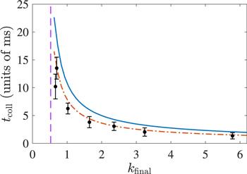
Figure 3. tcoll versus kfinal for N(0) = 6000, ainit = 10−4aB, and γ3 = 3 × 10⁻²⁷cm6 s–1. The filled circles (•) are the experimental data extracted from [2], the solid line represents the GST result, and the dash-dotted line is the GST result multiplied by a factor 12.8/17.5. The vertical dashed line marks kcri. |
4.2. Fluctuation assisted deferred collapses
In order to observe deferred collapses, we have to reduce the value of the three-body loss coefficient; otherwise, the atom number may decay too fast such that kfinal is significantly lowered and the collapse is suppressed. In figure 4, we plot the collapse time as a function of kfinal for N(0) = 6000, ainit = 10−4 aB, and γ3 = 10−28 and 10−29cm6 s–1. As can be seen, although ${k}_{\mathrm{cri}}^{(\mathrm{gpe})}\approx 0.52$ are roughly the same in both cases, ${k}_{\mathrm{cri}}^{(\mathrm{gst})}$ are now 0.505 and 0.495 for γ3 = 10−28 and 10−29cm6 s–1, respectively. In addition, it is seen that tcoll increases stepwise as kfinal gradually decreases. We point out that the three-body loss coefficient used here was also used in the earlier theoretical simulations [7] and is accessible in realistic experimental systems [4, 33].
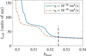
Figure 4. tcoll as a function of kfinal for γ3 = 10−28cm6 s–1 (solid line) and 10−28cm6 s–1 (dash-dotted line). Other parameters are N(0) = 6000 and ainit = 10−4 aB. The black dashed line marks the critical DIP obtained with GPE. |
To proceed further, we plot, in figure 5(a), N(t), NF(t), and NQ(t) for a typical deferred collapse with N(0) = 6000, ainit = 10−4 aB, afinal = −4.85 aB (kfinal = 0.5), and γ3 = 10−29cm6 s–1. Correspondingly, figure 5(b) plots the time dependence of the peak condensate density npeak and the entropy ${ \mathcal S }$ . As can be seen, once the collapse starts at around t ≈ 0.113 s, the dynamics behavior of the system becomes very similar to that of a direct collapse. Therefore, the feature that differs from a direct collapse lies in its dynamic behavior prior to the collapse. Particularly, as shown in figure 5(b), the peak density npeak oscillates for about 5/2 periods before the collapse. This oscillation corresponds to the breathing mode of the condensate and can be explained using the dynamical equation (32 ). In fact, for kfinal < 0.67, there exists a local minimum in the effective potential Veff. Thus after the scattering length is quenched, σ starts to oscillate around the equilibrium width. The oscillation frequency can be analytically obtained by linearizing equation (32 ), which gives rise to the period of the breathing mode38 ) yields Tbreathing ≈ 42 ms, which is in good agreement with numerical simulations. Following this analysis, because the density of the condensate attains the highest value at times that are odd multiples of Tbreathing/2, the tcoll–kfinal curve (figure 4) is naturally of the stepwise shape. Accompanying the density oscillation of the condensate, the number of fluctuated atoms also oscillates. In particular, at t ≈ 80 ms, NF can be as large as 1000 and it becomes even larger close to the tcoll. These fluctuated atoms originate from two mechanisms, i.e., the decay-induced decoherence and the attractive interaction-induced squeezing. Because, as shown in equation (11 ), the fluctuated atoms amplify the attractive interaction [23], collapse can then be induced when the number of atoms in the fluctuations becomes sufficiently large. As shown in figure 5(a), it should be noted that, among the fluctuated atoms, there are only a small fraction of atoms in the pure squeezed state (quantum depletion). Finally, once the collapse is initiated, the dynamical behavior of the gas, as shown in figures 5(b) and (c) for npeak, ${ \mathcal S }$ , and g(2)(r, r), is very similar to that of a strong collapse, which again suggests that fluctuations should be considered for the studying of the collapse dynamics.
$\begin{eqnarray}{T}_{\mathrm{breathing}}={T}_{\mathrm{ho}}{\left(\displaystyle \frac{1}{{a}_{\mathrm{ho}}^{2}}+\displaystyle \frac{3{a}_{\mathrm{ho}}^{2}}{{\sigma }_{0}^{4}}-8\displaystyle \frac{{k}_{\mathrm{final}}}{\sqrt{2\pi }}\displaystyle \frac{{a}_{\mathrm{ho}}^{2}}{{\sigma }_{0}^{5}}\right)}^{-1/2}.\end{eqnarray}$
For parameters used in figure 5, equation (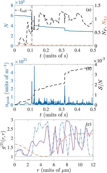
Figure 5. (a) N(t) (solid line), NF(t) (dashed line), and NS,1(t) (dash-dotted line). (b) Time dependence of the peak density (solid line) and the entropy per atom (dashed line). (c) The second-order correlation function g(2)(r, r) for t = 0 (dotted line), 0.1 (dashed line), 0.2 (dash-dotted line), 0.4 s (solid line). The parameters used here are N(0) = 6000, ainit = 10−4 aB, afinal = −4.85 aB, and γ3 = 10−29cm6 s–1. Correspondingly, the DIP is kfinal = 0.5. |
We would also like to point out that deferred collapse found here is stimulated by the fluctuations which are completely different from the delayed collapse previously predicted by Biasi et al [34]. Their study was based on the GPE with the atom decay mechanism being completely ignored. In addition, delayed collapses are induced by changing the shape of the initial condensates.
5. Conclusion and discussion
In conclusion, we have studied the collapse dynamics of a Bose–Einstein condensate using GST. Compared to the coherent-state-based GPE approach, fluctuations are properly treated at the mean-field level. It has been shown that the presence of the fluctuations leads to a critical interaction strength that is slightly smaller than that predicted by GPE. Moreover, the calculation of the fluctuated atoms, the entropy, and the second-order correlation function showed that the collapsed gas significantly deviated from a pure state. It is therefore inappropriate to treat the collapsed atom as a pure coherent state, although the calculation for atom number of the collapsed condensate does not appear to have much difference. In our future works, we shall revisit the d-wave collapse of dipolar condensates [35] and study the dynamical formation of quantum droplets in both dipolar and binary condensates [36, 37].