


1. Introduction
The most advanced models to describe atomic nuclei are those where all nucleons are active and where all inter-particle correlations are included. These methods are called ab initio, because only the form of the nuclear Hamiltonian is postulated at first so that nuclear many-body states are exact eigensolutions of the associated Schrödinger equation in principle. In practice, this means that many-body eigenstates can be calculated up to a margin that can be specified during the construction of the Hamiltonian. It has been possible to develop ab initio nuclear models because present theoretical interactions between nucleons are nowadays sufficiently accurate to reproduce the physical observables of few-body systems, where the three-body force can be included [1, 2]. Indeed, three-body forces are inherent of the nuclear interaction. They are responsible for the saturation of nuclear matter and they have been shown to exist at several orders of any effective field theory for nucleon.
However, despite the relatively direct and simple theoretical nature of ab initio nuclear models, their applications in numerical calculations are far from obvious. The most important problem is the hard core repulsion between nucleons, which prevents from using an independent-particle wave function as a starting point. A practical solution is to use equivalent low-energy inter-nucleon interactions, which remove the high-energy components of the nuclear Hamiltonian, while still reproducing the two-nucleon observables up to about 300 MeV [1, 2]. Nevertheless, model space dimensions grow very rapidly with the number of valence nucleons, as their increase is combinatorial. In fact, only nuclei bearing fewer than about 15 nucleons can be numerically treated with no-core–shell model (NCSM) [3].
Due to these theoretical and practical conundrums, it has then become clear that another route should be followed if one aims at considering heavier nuclei with ab initio shell model methods. A powerful idea is not to consider the initial Hamiltonian, but, on the contrary, to transform it so that a relatively small number of configurations is necessary to diagonalize it. One can cite for that matter the in-medium similarity renormalization group (IMSRG), which decouples particle-particle and hole-hole configurations so that a simple Hartree–Fock (HF) or Hartree–Fock–Bogoliubov ansatz can give a quasi-exact energy at a given flow parameter with the renormalized Hamiltonian [4–8]. Another method for transforming the initial Hamiltonian in order to be able to treat heavier nuclei is the many-body perturbation theory (MBPT), where an effective Hamiltonian is calculated perturbatively from the initial realistic Hamiltonian in small model spaces [9, 10].
Even though the latter numerical approaches allowed to greatly improve the number of nuclei that can be treated with ab initio methods, they still rely on the use of bases of square-integrable states, so that a precise calculation of halo and resonance nuclei is precluded. An alternative ab initio theoretical approach must then be implemented, which includes continuum coupling. Hence, one has generalized the Gamow shell model (GSM) [11] to ab initio frameworks, namely the no-core Gamow shell model (NCGSM) [12] and GSM with $\hat{\bar{Q}}$ -box method [13]. Indeed, GSM allows for the description of weakly bound and unbound states, because continuum coupling is included at basis level, while inter-nucleon correlations are present via configuration mixing [11].
Several calculations have been made in ab initio GSM and it is the object of this review to give a short description of its most important applications. For this, we will shortly present the basics of the one-body Berggren basis expansion in section 2 , as it is fundamental to formulate GSM. We will then focus on the numerical methods used to diagonalize the GSM matrix in section 3 , as the numerical problems met therein are different from those of the shell model using the harmonic oscillator basis. Then, we will quickly present the theory of NCGSM in section 4 , and its first applications afterward, i.e. the unbound nucleus 5He in section 5 , A = 3, 4 unbound nuclei in section 6 , and the oxygen and fluorine chains in section 7 , where the NCGSM Hamiltonian is transformed via MBPT to obtain GSM with $\hat{\bar{Q}}$ -box method. A conclusion will be made in section 8 .
2. Berggren basis and completeness relations
Many-body resonance wave functions are expanded on a basis of complex-energy independent-particle states in GSM. Thus, the completeness relation of complex-energy one-body eigenstates is fundamental and will be firstly depicted. For this, one has to consider the standard real-energy completeness relation generated by a one-body Hermitian Hamiltonian, i.e. the Newton completeness relation [14]:
$\begin{eqnarray}\sum _{n}{u}_{n}(r){u}_{n}(r^{\prime} )+{\int }_{0}^{+\infty }{u}_{k}(r){u}_{k}(r^{\prime} )\,{\rm{d}}k=\delta (r-r^{\prime} ),\end{eqnarray}$
where un(r) are the bound states and real-energy scattering states uk(r) run over the positive real-k axis.Let us now deform the integration contour of equation (1 ) into the complex k-plane in order for complex-energy states to explicitly appear, as shown in figure 1.
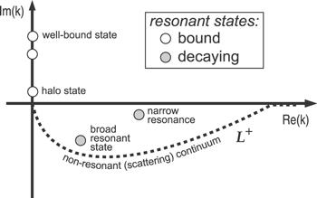
Figure 1. Representation of the complex k-plane, showing the positions of bound states, well bound or of halo character (empty disks) and resonances, narrow or broad (grey filled disks). L+ is the contour representing the non-resonant continuum. The Berggren completeness relation involves the bound states, resonance states lying between L+ and the real k-axis, and the scattering states on L+ (from [35]). |
Following the complex integration Cauchy theorem, one obtains:${u}_{k}(r){u}_{k}(r^{\prime} )$ lying between the real k-axis and the L+ complex contour. The Berggren completeness relation [15] follows immediately:
$\begin{eqnarray}\begin{array}{l}-{\displaystyle \int }_{0}^{+\infty }{u}_{k}(r){u}_{k}(r^{\prime} )\,{\rm{d}}k+{\displaystyle \int }_{{L}^{+}}{u}_{k}(r){u}_{k}(r^{\prime} )\,{\rm{d}}k\\ \quad =\,2{\rm{i}}\pi \sum _{{k}_{n}}\mathrm{Res}{\left({u}_{{k}_{n}}(r){u}_{{k}_{n}}(r^{\prime} )\right)}_{k={k}_{n}},\end{array}\end{eqnarray}$
where kn are the poles of $\begin{eqnarray}\sum _{n}{u}_{n}(r){u}_{n}(r^{\prime} )+{\int }_{{L}^{+}}{u}_{k}(r){u}_{k}(r^{\prime} )\,{\rm{d}}k=\delta (r-r^{\prime} ),\end{eqnarray}$
where un(r) are now the bound states and resonances present between the real k-axis and the L+ contour now consists of complex-energy scattering states uk(r) defined in the complex k-plane. All bound, resonance and scattering states un(r) and uk(r) are generated by the same basis potential.Equations (1 ), (3 ) are two completeness relations differing by way of their domain of definition. Indeed, equation (1 ) is similar to the Fourier transform as only bound states can expanded from the Newton completeness relation [14]. Conversely, equation (3 ) allows for the expansion of bound states and resonance states whose complex momentum is situated between the L+ contour and the real k-axis [15].
In order to be used in numerical calculations, equation (3 ) must be discretized, which is most efficiently performed with the Gaussian quadrature [11]:${u}_{{k}_{i}}(r)={u}_{n}(r)$ if it is a resonant state and ${u}_{{k}_{i}}(r)=\sqrt{{w}_{k}}{u}_{k}(r)$ if it is a discretized scattering state of momentum ki = k and Gaussian weight wk. The renormalization of discretized scattering states, depending on Gaussian weight, is necessary for one-body bound, resonance and scattering states to be treated on the same footing [11].
$\begin{eqnarray}\sum _{i=1}^{N}{u}_{{k}_{i}}(r){u}_{{k}_{i}}(r^{\prime} )\simeq \delta (r-r^{\prime} ),\end{eqnarray}$
where N is the total number of used resonant and discretized scattering states, Equation (4 ) is formally identical to the standard completeness relation in a discrete basis so that Slater determinants of the many-body Berggren basis are straightforward to generate. However, as the formalism of Gamow states is non-Hermitian, the obtained Hamiltonian matrix H is complex symmetric. New numerical methods then had to be devised to solve the eigenproblem specific to the GSM Hamiltonian matrix.
3. Numerical implementation of the Gamow shell model
3.1. Calculation of two-body matrix elements with the Berggren basis
Two-body matrix elements are straightforward to calculate with a basis of harmonic oscillator states. For this, one firstly evaluates nuclear matrix elements in relative coordinates with harmonic oscillator states, as the nuclear Hamiltonian is defined with the relative coordinates of the interacting nucleons. Then, one calculates the nuclear matrix elements in laboratory coordinates, which are necessary as Slater determinants are defined in the laboratory frame. This is conveniently done using the Talmi-Brody-Moshinsky transformation [16].
However, one cannot use the Talmi-Brody-Moshinsky transformation with the Berggren basis. In fact, a generalization of the Talmi-Brody-Moshinsky transformation to arbitrary bases exists and consists of the vector brackets method [17–19]. Unfortunately, it is of little practical use, as it leads to very time-consuming calculations. The reason for it is that the finite sums entering the Talmi-Brody-Moshinsky transformation become two-dimensional integrals with vector brackets [17–19]. Added to this difficulty, Dirac delta and Heaviside functions enter vector brackets, whose non-analytical character in the complex plane even complicates the extension of vector brackets to complex-energy states.
A new theoretical method clearly had to be devised for the numerical evaluation of nuclear matrix elements with the Berggren basis. For this, one has to rely on the fundamental property of the nuclear interaction in halo and resonance many-body states, which is its localized character in the vicinity of the considered nucleus. Indeed, it implies that an expansion of the nuclear interaction in a basis of harmonic oscillator states will converge rapidly, even though the many-body nuclear states of interest are either very extended in space (halos) or even diverge therein (resonances).
For simplicity, we will present the harmonic oscillator expansion method for a two-body interaction. Generalization to three-body, four-body,... interactions is straightforward. Let us represent the matrix elements of the two-body nuclear interaction $\hat{V}$ in the Berggren basis with a finite number of harmonic oscillator states [20]:${N}_{\max }$ is the number of used harmonic oscillator states and where greek (Latin) letters refer to harmonic oscillator (Berggren basis) states. As the action of the nuclear interaction is localized, one can indeed assume that $\hat{V}$ can be reliably reproduced with a fairly small value for ${N}_{\max }$ . The two-body matrix elements appearing on the right-hand side of equation (5 ) only involve harmonic oscillator states, so their evaluation is straightforward using the Talmi-Brody-Moshinsky transformation. Moreover, Berggren basis states only appear in overlaps of the form $\left\langle a| \alpha \right\rangle $ , i.e. in one-dimensional integrals of the products of Berggren basis and harmonic oscillator states. As harmonic oscillator states decrease like Gaussians when r → + ∞ and as Berggren basis states can at most increase exponentially in modulus therein, these overlaps are always well defined and converge rapidly when r → + ∞.
$\begin{eqnarray}\left\langle {ab}| \hat{V}| {cd}\right\rangle =\sum _{\alpha \beta \gamma \delta }^{{N}_{\max }}\left\langle \alpha \beta | \hat{V}| \gamma \delta \right\rangle \left\langle a| \alpha \right\rangle \left\langle b| \beta \right\rangle \left\langle c| \gamma \right\rangle \left\langle d| \delta \right\rangle ,\end{eqnarray}$
where As a demonstration of the effectiveness of the harmonic oscillator expansion method, we considered the 18O nucleus with an 16O core [20]. The 18O wave functions then consist of two valence nucleons, so that GSM calculations can be quickly effected. The used nuclear interaction consists of the N3LO realistic interaction, renormalized with the Vlow−k method using a cut-off momentum Λ = 1.9 fm−1 [20].
The convergence of the energies of the ground and excited states of 18O nucleus is depicted in table 1. Convergence occurs for the rather small value ${n}_{\max }\sim 10$ , and even for resonance states, where one can also see the fast convergence of the imaginary part of energies, proportional to widths.
Table 1. Convergence of the real and imaginary parts of energies (E) of the |
| | | | | | | ||
|---|---|---|---|---|---|---|---|
| | E | E | E | E | E | Re[E] | Im[E] |
| 4 | −12.225 | −8.438 | −12.1398 | −10.0488 | −11.0641 | −1.4373 | −0.8275 |
| 6 | −12.226 | −8.498 | −12.1465 | −10.0830 | −11.0907 | −1.4292 | −0.7600 |
| 8 | −12.228 | −8.499 | −12.1452 | −10.0853 | −11.0922 | −1.4380 | −0.7405 |
| 10 | −12.229 | −8.499 | −12.1450 | −10.0857 | −11.0921 | −1.4400 | −0.7390 |
| 12 | −12.228 | −8.499 | −12.1453 | −10.0858 | −11.0923 | −1.4393 | −0.7401 |
| 14 | −12.228 | −8.499 | −12.1453 | −10.0858 | −11.0923 | −1.4394 | −0.7401 |
| 16 | −12.228 | −8.499 | −12.1453 | −10.0858 | −11.0923 | −1.4394 | −0.7401 |
| 18 | −12.228 | −8.499 | −12.1453 | −10.0858 | −11.0923 | −1.4394 | −0.7401 |
| 20 | −12.228 | −8.499 | −12.1453 | −10.0858 | −11.0923 | −1.4394 | −0.7401 |
Apparently, the calculation of Coulomb two-body matrix elements with the Berggren basis still remains problematic. Indeed, the Coulomb interaction is of infinite range, so that equation (5 ) cannot be directly applied for that matter. The solution to this problem relies on the fact that the Coulomb interaction must behave as (Z − 1)/r at large distances. Thus, one can rewrite the Coulomb interaction ${\hat{V}}_{\mathrm{Coul}}$ as ${\hat{U}}_{\mathrm{Coul}}(Z-1)+({\hat{V}}_{\mathrm{Coul}}-{\hat{U}}_{\mathrm{Coul}}(Z-1))$ , where ${\hat{U}}_{\mathrm{Coul}}(Z-1)$ is a given Coulomb potential of charge Z − 1. The interest of this decomposition is that ${\hat{V}}_{\mathrm{Coul}}-{\hat{U}}_{\mathrm{Coul}}(Z-1)$ is of short-range character so that it can be expanded using equation (5 ). The one-body part ${\hat{U}}_{\mathrm{Coul}}(Z-1)$ poses no problem, as it is spherical and hence can be directly included in the generating potential of the Berggren basis.
As a consequence, the calculation of two-body matrix elements with the Berggren basis is affected by separating its finite-range and infinite-range parts and by introducing a harmonic oscillator expansion afterward (see equation (5 )). It only relies on the Talmi-Brody-Moshinsky transformation and quickly converging one-dimensional overlap integrals, so that it is convenient to use in practical applications.
3.2. Determination of eigenvalues in Gamow shell model: the overlap method.
In order to diagonalize the standard shell model matrices, the Lanczos method is widely employed, as it allows for the determination of low-energy nuclear states without having to fully diagonalize the Hamiltonian matrix [21]. However, even though the Lanczos method can be straightforwardly extended to complex symmetric matrices, it cannot be applied directly in GSM, because resonance A-body states are surrounded by many scattering A-body states. Indeed, the low-energy spectrum obtained in GSM with the Lanczos method consists of bound, resonance and scattering eigenstates, which cannot be separated out.
In fact, it is impossible to know whether a GSM eigenstate is a resonance or scattering state from the knowledge of its eigenenergy only. Only bound states can be identified unambiguously from their eigenenergies, which are always negative. Hence, one has to determine the resonant or scattering nature of eigenstates, even though one does not have access to their asymptotic properties. A solution to this problem could be devised with the overlap method [22], which is performed in two steps:
| • | The Hamiltonian matrix is diagonalized at pole approximation level, i.e. with a basis of Slater determinants where only resonant one-body states are occupied. One then obtains the |
| • | The full Hamiltonian matrix is diagonalized, i.e. with a basis of Slater determinants generated by the complete Berggren basis, with both resonant and scattering one-body states. The sought GSM eigenstate |
As the occupation of non-resonant basis Slater determinants is small compared to pole configuration components, this method works very well in practice. Note that the Jacobi-Davidson method [23] is used at this level instead of the Lanczos method for Hamiltonian diagonalization. Indeed, as resonance energies are interior eigenvalues, the Jacobi-Davidson method can efficiently provide associated eigenstates, in contrast to the Lanczos method, well suited for extremal eigenvalues [21, 24].
3.3. Natural orbitals
In order to diminish the size of Hamiltonian matrices, it is possible to use optimized one-body states. While the HF method provides by definition the best basis-generating potential [25], the obtained one-body basis states are not optimal because inter-nucleon correlations are neglected in the HF potential. In fact, the optimal one-body states are those with which nucleon occupation is maximized in the considered many-body eigenstate, which are called natural orbitals [26].
Natural orbitals are the eigenvectors of the scalar one-body density matrix [26], whose matrix elements read:$\left|{\rm{\Psi }}\right\rangle $ is the sought many-body state. As $\left|{\rm{\Psi }}\right\rangle $ is not known, one uses instead an approximate eigenstate $\left|{{\rm{\Psi }}}_{{app}}\right\rangle \simeq \left|{\rm{\Psi }}\right\rangle $ , calculated in a truncated model space generated by the Berggren basis, in which numerical calculations are tractable. Note that, contrary to well bound systems, natural orbitals in unbound many-body states are unbound as well. Added to that, they contain sizable scattering components, issued from the continuum coupling present in $\left|{{\rm{\Psi }}}_{{app}}\right\rangle $ . Consequently, the use of natural orbitals is not restricted to bound NCGSM eigenstates, but is also of practical interest for resonance NCGSM eigenstates.
$\begin{eqnarray}{\rho }_{{mn}}=\left\langle {\rm{\Psi }}| {\left[{a}_{m}^{\dagger }{\tilde{a}}_{n}\right]}_{0}^{0}| {\rm{\Psi }}\right\rangle ,\end{eqnarray}$
where m, n are the indices of the one-body states of the used Berggren basis and As natural orbitals are defined with respect to the sought many-body state, only a few natural orbitals are necessary to accurately represent a given partial wave. One has seen in practice that typically 5–7 natural orbitals per partial wave have to be used, which is to be compared to the 30–50 discretized scattering states necessary when using the Berggren basis [27]. Due to the quickly increasing matrix dimensions with the number of basis one-body states, the size of matrices can be decreased by several orders of magnitude when replacing Berggren basis states by natural orbitals. Consequently, calculations impossible to do with the Berggren basis can be performed without truncations with natural orbitals.
However, if the number of valence nucleons and/or valence states becomes too large, even the use of natural orbitals is not sufficient. In fact, it is necessary to resort to other diagonalization methods as the Jacobi-Davidson method [23] in this case. Hence, one has developed for that purpose the density matrix renormalization group method (DMRG), where the matrix-vector applications involving the full Hamiltonian matrix are avoided.
3.4. Diagonalization of very large Gamow shell model matrices with the density matrix renormalization group approach
DMRG is an iterative method that allows diagonalizing Hamiltonians without having to explicitly store their configuration interaction matrix. For this, Hamiltonians are instead represented by bases where particles are increasingly correlated through a renormalization process, so that matrix dimensions to consider remain small, while their eigenvectors converge to those of the initial Hamiltonians. In fact, DMRG has become a standard method to solve the many-body problem in matter physics [28]. DMRG has been tested a few years ago in nuclear physics with the harmonic oscillator shell model, where it only found little success, however (see [29–32]). Convergence was noticed to be rather slow, as a large part of the total shell model space was needed in order for eigenenergies to converge. The reason for this situation is the large nucleon–nucleon correlations present in atomic nuclei. Indeed, DMRG converges the fastest when correlations are weak, even if numerous, as is the case in spin chains, where DMRG was introduced [33, 34].
Similarly, the nuclear many-body states studied in GSM are very good candidates for DMRG. Indeed, contrary to well-bound nuclei, correlations involving the numerous non-resonant configurations are weak, while the strong nuclear interaction is mainly acting among a few pole configurations. Consequently, nuclear states in GSM can be expected to converge more rapidly than well-bound nuclei with DMRG. However, DMRG was initially implemented for Hermitian Hamiltonians, so it was necessary to extend it to the complex symmetric case.
For that matter, the GSM valence model space is separated into two spaces: the first one, the A reference space, is generated by the one-body resonant states of the Berggren basis, while the second one, the B space, is built in the DMRG process, by adding one after the other the remaining scattering states of the Berggren basis (see figure 2). When dimensions become too large in the non-resonant space in DMRG, the Hamiltonian matrix is diagonalized, so that it provides an approximate nuclear eigenstate by using the overlap method (see section 3.2 ). At this level, the reduced density matrix is calculated and diagonalized, as its eigenvectors have been shown to be the closest to exact Hamiltonian eigenvectors [33, 34]. A new optimal basis space is then calculated from the Nopt eigenvectors of the reduced density matrix bearing the largest eigenvalues. All sub-operators associated with the Hamiltonian must then be recalculated, which then forms a DMRG step. Several ‘sweeps', i.e. inclusions of the same one-body basis states by enumerating several times all scattering basis states, are necessary in order to recapture the inter-nucleon correlations neglected in the previous renormalization processes.
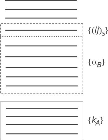
Figure 2. Simplified illustration of the DMRG method. The {kA} states come from the A reference space and the αB states belong to the B space. The shell (lj)s is added to the B space, which generates the new basis states {kA ⨂ {αB ⨂ (lj)s}}J (from [35]). |
The first application of DMRG in GSM was done in [35], where only valence neutrons were considered. The more general case of model spaces containing both valence protons and neutrons was introduced a few years later [36]. DMRG has been applied in light nuclei in the core+valence nucleon picture. The $3/{2}_{1}^{-}$ ground state and the $1/{2}_{1}^{-}$ first excited state of 7He were considered in [35], and the ground states of the 7Li and 8Li nuclei were studied afterwards in [36]. The fast convergence of DMRG in GSM is depicted in figure 3 for the 7He nucleus.
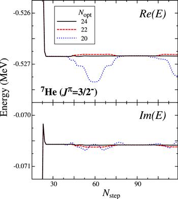
Figure 3. Convergence of the real and imaginary parts of the energy of |
4. No-core Gamow shell model
4.1. Hamiltonian and interaction
In ab initio approaches, and hence in NCGSM, the aim is to solve the A-body Schrödinger equation, where H is the intrinsic nuclear Hamiltonian:${\hat{V}}^{{NN}}$ , ${\hat{V}}^{{NNN}}$ , ... are realistic two-nucleon, three-nucleon ,... interactions. As is usually the case, the Hamiltonian $\hat{H}$ is restricted to the use of two and three-body interactions. Many-body interactions arise due to the rotation of the Hilbert space induced by IMSRG or MBPT transformations, for example. Only two-body interactions will be considered in the next applications.
$\begin{eqnarray}\hat{H}=\sum _{i=1}^{A}\displaystyle \frac{{{\boldsymbol{p}}}_{i}^{2}}{2m}-\displaystyle \frac{{{\boldsymbol{P}}}^{2}}{2{mA}}+\sum _{i\lt j}^{A}{\hat{V}}_{{ij}}^{{NN}}+\sum _{i\lt j\lt k}^{A}{\hat{V}}_{{ijk}}^{{NNN}}+\,...,\end{eqnarray}$
where In NCGSM, local or non-local interactions can be included, contrary to the Green's Function Monte Carlo approach, for example, where non-local potentials cannot be handled as Green's Function Monte Carlo are solved in coordinate space. Thus, a local interaction such as the Argonne ν18 potential [1], or a non-local interaction such as the CD-Bonn 2000 [2], as well as various chiral interactions, can be considered.
Softening techniques such as Vlow−k [37], similarity renormalization group [38, 39], or G-matrix approaches [9, 40], must usually be applied in order to be able to use bare nuclear interactions in small model spaces. This will be the case in the examples discussed in the next sections, where one uses the nuclear chiral interactions [41], renormalized with the Vlow−k technique, using a sharp momentum cutoff Λ ∼ 2 fm−1 in order to decouple the degrees of freedom of low and high momenta [42]. Note that, in principle, the microscopic potential and chiral interactions derived from effective field theory are different mathematical objects. However, as we do not deal with the nuclear interaction itself, but only with its application in GSM, we will not insist on this point.
4.2. Center of mass treatment
As in the harmonic oscillator shell model, a spurious center of mass excitations can appear in NCGSM. This arises because the number of physical degrees of freedom of the nucleus is 3A − 3, whereas the many-body wave function depends on A nucleons, and hence on 3A space coordinates. Thus, spurious center-of-mass motion arises due to the three redundant degrees of freedom.
The solution to this problem in the harmonic oscillator shell model has been known for a long time and consists of the application of the Lawson method [43]. For this, by using shell model spaces defined in full Nℏω space, the total wave function factorizes into $\left|{\psi }_{\mathrm{rel}}\right\rangle \otimes \left|{\psi }_{\mathrm{CM}}\right\rangle $ , where $\left|{\psi }_{\mathrm{CM}}\right\rangle $ is an eigenstate of the harmonic oscillator center of mass Hamiltonian [43]. However, the Lawson method cannot be extended in general to the NCGSM. Indeed, as $\left|{\psi }_{\mathrm{CM}}\right\rangle $ is localized in space, the former decomposition of the total wave function in relative and center of mass parts only applies to well-bound many-body states. In fact, an exact separation in relative and center of mass parts of NCGSM eigenstates cannot occur except in infinite model spaces.
Fortunately, it is not necessary for the NCGSM ground state wave function to be separated in relative and center of mass parts to reliably represent the exact many-body wave function in infinite space, which is due to the generalized variational principle [44, 45]. Indeed, similarly to the variational principle governing bound states, one can show that the eigenenergy of NCGSM ground states is stationary with respect to small changes of NCGSM space [44]. Thus, due to the intrinsic character of the Hamiltonian, eigenenergies converge to their exact value in infinite space when NCGSM model spaces are becoming larger, even in the absence of an exact separation in relative and center of mass parts. The difference between NCGSM eigenstates in truncated and infinite space can similarly be assumed to be small if the model space used is sufficiently large. The fundamental advantage of this method is that it can be applied to many-body unbound states. This will be the method used for the next applications, dedicated to the study of the resonance ground states of 5He and 3,4n.
Note, however, that the generalized variational principle does not apply to excited states, as we have no guarantee that an obtained excited state is not a repetition of the ground state with a different center of mass motion. In fact, how to correct in the general case for center-of-mass motion in NCGSM is still an open question.
5. Ab initio description of the 5He resonance nucleus
5.1. 5He resonance properties
Due to the well-unbound character of both its ground and first excited states, the ab initio description of 5He is a difficult task. Its resonance properties had been evaluated along with those of other resonance many-body states with the variational Monte-Carlo method in [46]. The associated nucleon-alpha scattering reaction had also been studied with the quantum Monte-Carlo method in [47]. As both halo and resonance many-body states can be calculated in NCGSM, the study of 5He is well-suited in the frame of NCGSM.
For that matter, as the width of 5He mainly comes from the neutron p3/2 partial wave, one will use the Berggren basis to expand this partial wave, where 0p3/2 is a one-body resonance state, of energy 1.193 MeV and width 1.267 MeV. The neutron s1/2 and p1/2 partial waves are chosen to be real, where the p1/2 partial wave consists of a real-energy contour only, while the s1/2 contour must be complemented by the well-bound 0s1/2 pole state, of energy equal to –24 MeV. As other partial waves add binding energy to the 5He system without changing its asymptotic behavior, they are represented with harmonic oscillator basis states.
Due to the very large dimensions occurring in the NCGSM description of 5He, one has used DMRG to diagonalize the NCGSM Hamiltonian (see section 3.4 ). Note that the dimension of the DMRG Hamiltonian matrix to diagonalize is 105, which is much smaller than the NCGSM Hamiltonian matrix in a basis of Slater determinant, which is close to 3 × 10⁹.
Results are shown in the upper part of figure 4, for which one has used Λ = 1.9 fm−1. The obtained energy for the ground state of 5He is ${\mathfrak{R}}(E)=-26.31\,\mathrm{MeV}$ , hence one MeV too high with respect to experimental data [48]. From the NCGSM energies of the ground states of 4He and 5He, one can determine the 5He resonance to be at neutron separation energy 1.17 MeV, which is less than 500 keV away from the experimental energy of 0.735 MeV. Presumably, the binding energy lacking in 4He and 5He could be attributed to the missing three-nucleon forces. The chiral interaction used might also play a role. This would explain the better reproduction of the neutron separation energy of 5He compared to its total binding energy.
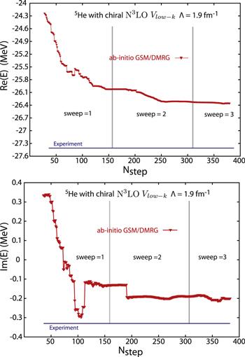
Figure 4. Convergence of the real and imaginary parts (upper and lower parts, respectively) of 5He ground state energy, calculated with the density matrix renormalization group, is shown as a function of the number of iterations, also called sweeps. Experimental data are also provided [48] (from [12]). |
Resonance properties are extracted differently according to the model used [49–51]. One can either use the Lane and Thomas prescription to determine the energy and width of resonance from the conventional R-matrix approach on the real axis [52], or use the extended R-matrix approach [50, 51], where the complex poles of the S-matrix provide the energy and width of the resonance from their real and imaginary parts. As NCGSM is a numerical method where many-body S-matrix poles are calculated, the definition of resonances of the extended R-matrix approach is closest to that of NCGSM. The latter extraction method approach determines the position of the 3/2− ground state of 5He at an energy 0.798 MeV above the neutron threshold, while its width Γ is equal to 648 keV. The width of the ground state of 5He is provided by the imaginary part of the 5He ground state energy (see the lower part of figure 4). The obtained imaginary part of the energy of the ground state of 5He is ${\mathfrak{I}}(E)=-0.2\,\mathrm{MeV}$ , i.e. Γ = 400 keV. As for total binding energy, but to a lesser extent, the difference between the widths arising from NCGSM and experimental data might be due to missing many-body forces, or to the chiral interaction itself.
In order to verify these assumptions, the 3/2− ground state of 5He has been recalculated in NCGSM using slightly different Hamiltonian parameters. For this, one has used two different Vlow−k renormalizing momenta, which are Λ = 1.9 fm−1 and 2.1 fm−1. For this comparative study, a smaller model space has been utilized, where only the neutron p3/2 partial wave is represented by Berggren basis states, other one-body basis states being harmonic oscillator states. Added to that, one truncated the NCGSM space so that a maximum of four nucleons in the non-resonant continuum is accepted in the basis of Slater determinants. The NCGSM is then sufficiently small to be able to use the Jacobi-Davidson diagonalization method [11, 23].
With Λ = 1.9 fm−1, the obtained energy for 4He is equal to −27.386 MeV, while that of 5He is E = −25.825 MeV, with a width Γ = 370 keV. These results are close to the DMRG results and hence justify a posteriori the use of truncated model spaces. When the Λ momentum has the value 2.1 fm−1, one obtains instead −26.06 MeV for the binding energy of 4He, whereas the total binding energy and width of 5He are E = −23.90 MeV and Γ = 591 keV, respectively. Thus, the neutron separation of the 5He ground state is 2.15 MeV above the α + n decay threshold. Hence, clearly, the resonance properties of the ground state of 5He largely depend on the interaction used, which explains the discrepancies encountered with respect to experimental data.
The position of the energy of the 5He resonance ground state and its associated width, obtained from R-matrix theory, are listed in table 2. One can see that the values obtained are rather different from each other, which reflects the broad character of the 5He resonance ground state.
Table 2. The DMRG results for the energy and width of the 5He ground state obtained in NCGSM are compared to experimental data, determined from several R-matrix procedures. Shown energies are provided with respect to the α + n decay threshold (adapted from [12]). |
5.2. Radial overlap integral and asymptotic normalization coefficient
The reproduction of the energy and width of a many-body resonance state is not sufficient to assess the quality of the many-body wave function. The asymptotic behavior of a many-body resonance state can be quantitatively studied by considering the overlap function and the associated asymptotic normalization coefficient (ANC) (see [53] for definition and details). The overlap function is a radial function providing information about nuclear structure in a many-body state [46, 54]. As we are considering the ab initio description of 5He, we will show the overlap function in the context of the reaction 4He${}_{{0}^{+}}$ + n → 5He${}_{3/{2}^{-}}$ :${a}_{i,{\ell }=1,j=3/2}^{\dagger }$ creates a neutron state in a p3/2 one-body state of the Berggren basis and ui,ℓ=1,j=3/2(r) is the p3/2 radial basis wave function. As the ground state of 5He decays almost uniquely through the neutron p3/2 channel, it is sufficient to consider the radial overlap integral of equation (8 ) to determine the asymptotic behavior of the ground state of 5He. The precision of the overlap function of equation (8 ) depends on two factors: the completeness of the neutron p3/2 partial wave, which is represented by the Berggren basis, on the one hand, and the accurate reproduction of the one-neutron separation energy S1n, on the other hand.
$\begin{eqnarray}\begin{array}{l}{{\rm{I}}}_{{\ell }=1,j=3/2}(r)=\displaystyle \frac{1}{2}\\ \quad \times \,\displaystyle \sum _{i}\left\langle \widetilde{{}^{5}{\mathrm{He}}_{3/{2}^{-}}}\parallel {a}_{i,{\ell }=1,j=3/2}^{\dagger }{\parallel }^{4}{\mathrm{He}}_{{0}^{+}}{u}_{i,{\ell }=1,j=3/2}(r)\right\rangle ,\end{array}\end{eqnarray}$
where The radial overlap integral for 4He${}_{{0}^{+}}$ + n →5He${}_{3/{2}^{-}}$ is shown in figure 5, where the NCGSM calculation is performed using the chiral N3LO interaction [41] with Λ = 1.9 fm−1. One can determine the value of the ANC (denoted by C in the following) by fitting the radial overlap integral in the asymptotic region by a Hankel function (see figure 5). Indeed, the ANC is the multiplicative coefficient of the fitting Hankel function and has been found equal to C = 0.197 fm−1/2.
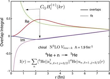
Figure 5. The radial overlap integral for 4He |
Note that results heavily depend on the cutoff parameter Λ, because S1n = −1.56 MeV and S1n = −2.15 MeV for Λ = 1.9 fm−1 and 2.1 fm−1, respectively (see table 3). Indeed, associated ANCs are respectively equal to 0.197 fm−1/2 and 0.255 fm−1/2 in the latter cases.
Table 3. NCGSM results calculations of the one-neutron separation energy S1n and spectroscopic amplitude |
| Λ fm−1 | S1n (MeV) | |
|---|---|---|
| 2.1 | −2.15 | 0.812 |
| 1.9 | −1.56 | 0.787 |
| 1.5 | −1.38 | 0.774 |
A convenient test of the accuracy of the ANC is the relation existing between the ANC and the resonance width Γ (see [46, 53, 55] and references cited therein):$\left(k=\sqrt{2{{mS}}_{1{\rm{n}}}/{{\hslash }}^{2}}\right)$ of the one-neutron separation energy S1n. Note that, even though k is a complex number in general, its imaginary part can be neglected if Γ ≪ ∣S1n∣.
$\begin{eqnarray}C=\sqrt{\displaystyle \frac{{\rm{\Gamma }}\mu }{{{\hslash }}^{2}{\mathfrak{R}}(k)}},\end{eqnarray}$
where μ is the effective mass and k is the linear momentum Using equation (9 ), one obtains ΓANC = 311 keV and ΓANC = 570 keV for Λ = 1.9 fm−1 and 2.1 fm−1, respectively. These values for the widths are consistent with those obtained from the imaginary part of energies in NCGSM (see section 5 ), as the 10%–15% difference between NCGSM widths and ΓANC can be traced back to the rather broad character of the ground state width of 5He, implying that equation (9 ) is only approximate therein.
The spectroscopic factor is the norm of the square of the radial overlap integral ${{\rm{I}}}_{{\ell }j}{\left(r\right)}^{2}$ :
$\begin{eqnarray}{S}_{{\ell }j}={\int }_{0}^{+\infty }{{\rm{I}}}_{{\ell }j}{\left(r\right)}^{2}\,{\rm{d}}r,\end{eqnarray}$
While Sℓj is not an observable [56], its value nevertheless provides important information about nuclear structure (see [54, 57–61] for spectroscopic factor calculations in various situations). Indeed, a large value for the spectroscopic factor indicates that the nuclear many-body function has a single-particle character, whereas a small value, in this case, would depict a highly correlated structure.An interesting tendency of spectroscopic factors as a function of the momentum cut-off Λ has been found in 4He/5He pairs calculated in NCGSM (see table 3). Indeed, by decreasing the momentum cut-off Λ, or, equivalently, by softening the interaction, one can see that ${S}_{{p}_{3/2}}^{1/2}$ departs more and more from unity. This shows that one cannot infer a priori any single-particle character of the ground state of 5He, i.e. of one neutron occupying a 0p3/2 resonance state in the mean field potential generated by the 4He core. On the contrary, the 5He wave function content heavily depends on the Λ value used in the Hamiltonian.
6. A = 3,4 unbound nuclei
6.1. Trineutron and tetraneutron in the auxiliary potential method
The trineutron and tetraneutron systems are not well known despite their small number of nucleons (see [62] and references therein). The study of multi-neutron systems, which are broad resonances, is difficult with standard ab initio methods, as the latter are tailored for well-bound atomic nuclei [63, 64].
Hence, NCGSM is the tool of choice to study multi-neutron systems, as continuum coupling and inter-nucleon correlations can be both included in this framework. This has been done firstly in [65] for tetraneutron, where, unfortunately, calculations were still incomplete, as they could be performed only in truncated model spaces or with overbinding interactions so that one could not make any definite conclusion. Consequently, multi-neutron systems have been reconsidered in [62] in the context of NCGSM, where converged results could be obtained in physical situations, albeit in truncated spaces.
The main issue to solve in the first place is the identification of the resonance states of multi-neutron systems. Indeed, multi-neutron systems are so dilute that the overlap method presented in section 3.2 is no longer sufficient to extract resonances from the many-body spectrum made almost exclusively of scattering states of complex energy. As a consequence, we introduced auxiliary potentials to confine neutrons in an external trap. This method was initially introduced in the quantum Monte-Carlo framework [64, 66]. For this, one adds to the ab initio Hamiltonian of equation (7 ) an auxiliary Woods–Saxon potential of potential depth Vaux, which will vary from a finite negative value to zero. As multi-neutron systems become well bound for sufficiently large negative values of Vaux, the calculation of Hamiltonian eigenstates is stable therein when applying the overlap method (see section 3.2 ). From this starting point, one can follow Hamiltonian eigenstates adiabatically when Vaux → 0. It has been checked that this method provides nearly exact results for the dineutron system [67].
The ground states of the trineutron and tetraneutron will be calculated using the auxiliary potential method. The interaction used is the chiral two-body interaction N3LO [68] renormalized with Λ = 2.1 fm−1. The single-particle Berggren basis, possessing bound, resonance and scattering states, is generated by a standard Woods–Saxon potential [68]. One imposes either 3p-3h and 4p-4h truncations in NCGSM model spaces, i.e. only three or four neutrons can occupy non-resonant basis states in Slater determinants, respectively.
One also uses the so-called ‘large' model space, where basis Slater determinants are generated from s1/2, p3/2 Berggren basis states, as well as p1/2, f5/2, f7/2, g9/2 harmonic oscillator states. Alternatively, in the so-called ‘small' model space, Slater determinants are built using the same partial waves as in the ‘large' model space, but with the p1/2, d3/2, d5/2 and f5/2, f7/2, g9/2 partial waves represented by only two and one harmonic shells, respectively. Eigenenergies have been checked to vary smoothly vary when Vaux → 0, i.e. that no multi-neutron channel opens when Vaux decreases. Results for both the trineutron and tetraneutron in various model spaces are shown in figure 6.
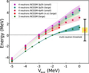
Figure 6. Energies and widths of the trineutron and tetraneutron systems as a function of the depth of the auxiliary Woods–Saxon potential. For tetraneutron calculations, NCGSM spaces with three particles at most in the non-resonant continuum, and without model space truncation, have been considered. Berggren or natural orbital (n.o.) bases have been used, while ‘small' or ‘large' denotes a model space where the number of basis shells has been reduced or not (see text for details). Tetraneutron width was decreased by a factor 3 for readability. Trineutron results are always obtained without model space truncation. The experimental data for tetraneutron (see [62]) are also shown (adapted from [68]). |
However, despite the progress made compared to [65], tetraneutron energies could not be reached in the ‘large' model space beyond the value of Vaux = −1.5 MeV. In fact, the physical region could be attained either in NCGSM truncated spaces, in ‘small' model spaces, denoted as 'small' in figure 6, or using 3p-3h truncations. Therefore, it is still necessary to rely on extrapolations to have an estimate of the energy and width of tetraneutron with realistic interactions.
The auxiliary potential method, used with the Jacobi-Davidson diagonalization technique (see figure 6) [23], and DMRG (see section 3.4 ) [62], both predict similar tetraneutron energy, which is close to 2.6 MeV. This energy lies within the range provided by experimental errors [62]. The width is estimated to be equal to 2.38 MeV from the extrapolation of the results obtained in the ‘large' model space with Vaux < − 1.5 MeV. Conversely, it was possible to obtain the trineutron ground state without model space truncation in the physical region. One obtained therein E3n = 1.29 and Γ3n = 0.91 MeV. One should recall, nevertheless, that these results are tentative, and hence not definitive and still subject to debate. For example, the results obtained with Faddeev–Yakubovsky techniques in [69] indicate that no n4 resonance can be produced from realistic nuclear interactions unless they are unphysically modified.
Interestingly, the energy and width of the trineutron are smaller than that of the tetraneutron (see figure 6), its energy still being larger than that of the dineutron. Consequently, it might be that the trineutron resonance might not be as broad as tetraneutron, which should be confirmed experimentally if it is the case.
6.2. A = 4 unbound isospin multiplet
Nuclei bearing four nucleons possess resonance states in their spectrum. Hence, they form good laboratories to test realistic nuclear interactions in nuclei far from stability with NCGSM. Of particular interest is the A = 4 T = 1 isospin multiplet formed by the first 2− states of 4H, 4He and 4Li. This isospin multiplet has unique features, because continuum coupling is maximal in unbound states, so that one can assess the influence of the Coulomb force in broad resonances and then quantitatively measure isospin symmetry breaking in this case.
The isospin symmetry in the considered A = 4 T = 1 multiplet states is indeed expected to be well broken. This is especially due to the Coulomb force [70–72], which acts very differently in 4H, 4He and 4Li. Indeed, both proton–proton and Coulomb forces are absent in 4H, whereas 4Li has no neutron-neutron interaction. Consequently, we studied the unbound spectrum formed by the first 2− states of the spectrum of 4H, 4He and 4Li with NCGSM in [45].
Results are shown in figure 7, where one presents many-body states in A = 3, 4 nuclei, along with the isospin triplet states calculated with NCGSM using the realistic interaction N3LO-SRG2.0, where SRG stands for similarity renormalization group. Both the ground states of 4H and 4Li are unbound and bear large particle-emission widths. The eigenstates of A = 3, 4 nuclei can be seen to be well described in figure 7. The broad character of the T = 1 isospin triplet states of A = 4 nuclei is reproduced [70]. In particular, the calculated energy of the T = 1 Jπ = 2− excited state in 4He is close to that arising from an R-matrix analysis [71]. Indeed, the 4He 2− excited state is found to be 22.03 MeV above the 4He ground state. This result agrees with the experimental value of [70], which is equal to 22.5 ± 0.3 MeV. Nevertheless, the width of the 4He 2− excited state obtained in the R-matrix analysis is about three times larger than in our calculation.
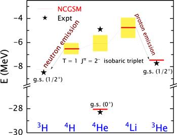
Figure 7. Unbound 2− states of T = 1 isospin multiplet of the A = 4 nuclei, calculated using NCGSM and the N3LO-SRG2.0 interaction. Experimental data come from [71, 90]. Dotted lines connect the T = 1 isobaric triplet states of A = 4 nuclei to guide the eye, while the obtained energies for A = 3 are also given for comparison. The experimental energy of the T = 1 Jπ = 2− state in 4He is deduced from the R-matrix analysis in [71] (from [45]). |
The calculations illustrated in figure 7 allow us to exhibit the isospin symmetry breaking occurring in the T = 1 isospin triplet states of A = 4 nuclei. One can see that the 2− state of 4H, which is also its ground state, is the lowest state in energy. The 4H isotope is more bound by about 0.5 and 1.7 MeV when it is compared to the 2− states of the same multiplet in 4He and 4Li, respectively. As could be expected, the width of the 2− excited state in 4He, equal to about 1.5 MeV, has a value in between those of 4H and 4Li.
In order to have a well-defined estimate of isospin symmetry breaking in the T = 1 triplet states, the isospin expectation value of their 2− analog states has been calculated. While the value of isospin in the ground states of 4Li and 4H ground states is equal to 1, that for the 2− excited state of 4He is equal to about 0.71. This suggests that isospin symmetry breaking is large in this state. Note that the isospin mixing occurring in the 2− excited state of 4He is consistent with experimental data [73, 74].
The presented NCGSM calculations of the A = 4 T = 1 isospin multiplet have clearly exhibited isospin symmetry breaking. While it originates from the Coulomb interaction and continuum coupling, it is difficult to disentangle both these effects, however.
7. Renormalization of realistic interactions in a finite model space using $\hat{\bar{Q}}$ -box method
In order to consider heavier systems than in NCGSM, while still dealing with realistic Hamiltonians, it would be useful to extend IMSRG [4–8] or MBPT [9, 10] to GSM, as one would reduce model space dimensions. Therefore, the extension of the $\hat{\bar{Q}}$ -box method has been implemented within the GSM framework, similarly to the harmonic oscillator shell model [75].
However, the generalization of the IMSRG and MBPT methods to GSM is not straightforward. Indeed, a caveat appears with the optimization of the single-particle basis, which does not exist in the harmonic oscillator shell model. It had been noticed that the many-body perturbation expansion entering the $\hat{\bar{Q}}$ -box method poorly converges with a Berggren basis arising from a Woods–Saxon potential [75]. The solution to this problem relies on the use of the HF potential of the Hamiltonian instead of a Woods–Saxon potential to generate the one-body basis. As many diagrams present in MBPT cancel out when a HF basis potential is utilized, the convergence of the $\hat{\bar{Q}}$ -box method is much faster, so that IMSRG and MBPT can be efficiently applied in GSM.
The $\hat{\bar{Q}}$ -box method is based on the separation of the many-body Hamiltonian of equation (7 ) into two parts, the one-body part ${\hat{H}}_{0}$ , which is then the Hamiltonian seen at zeroth-order, and a residual part $\hat{V}$ :${\hat{H}}_{0}$ is exactly represented by the HF potential of the Hamiltonian. A $\hat{\bar{Q}}$ -box folded-diagram calculation can then be performed in the basis generated by the same HF potential.
$\begin{eqnarray}\hat{H}={\hat{H}}_{0}+(\hat{H}-{\hat{H}}_{0})={\hat{H}}_{0}+\hat{V}.\end{eqnarray}$
Consequently, MBPT is based on the extended Kuo-Krenciglowa (EKK) method, which provides a quickly converging series of Hamiltonian powers [76]. However, it is derived with degenerate basis states, so it can hardly be used with the Berggren basis, as its one-body basis states all have different energies. Consequently, it is more convenient to use the EKK method generalized to nondegenerate basis states in order to obtain the effective Hamiltonian ${\hat{H}}_{\mathrm{eff}}$ [10, 77, 78].
The $\hat{\bar{Q}}$ -box method was initially applied in GSM calculations in [13]. We will then concentrate on its main results, i.e. the calculation of the spectra of isotopes of oxygen and fluorine with effective Hamiltonians ${\hat{H}}_{\mathrm{eff}}$ . For this, one uses the optimized chiral interaction NNLOopt in the nuclear Hamiltonian, as it can describe many observables of nuclear structure without having to recur to three-body forces [79].
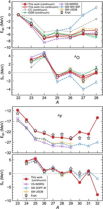
The GSM ground-state and single-neutron separation energies, denoted as Egs and Sn, respectively, are illustrated in figure 8 and compared to experimental data and theoretical calculations issued from other models. One can see that the neutron dripline is reproduced for oxygen isotopes in shell model calculations when three-nucleon forces are included [80] (labeled ‘SM NN+3NF' in figure 8). However, the quality of results strongly depends on the model used beyond the neutron dripline. This happens to be the case because the coupling to the decay channels must be included for the neutron dripline to be correctly predicted [81, 82]. Open decay channels and particle continuum are indeed not included in the shell model with two-nucleon and three-nucleon forces [80], shell model USDB [83] and valence-space IMSRG calculations [84] (see respectively curves labeled ‘SM NN+3NF', ‘SM USDB' and ‘VM-IMSRG' in figure 8). Conversely, GSM utilized with MBPT and two-body interactions (labeled ‘This work (continuum)' in figure 8) correctly provides the location of the neutron dripline for oxygen isotopes. As a consequence, one can obtain a good description of the 25,26O isotopes with GSM, even though they are situated beyond the neutron dripline (see the upper panel in figure 8). However, the effects arising from three-nucleon forces and couplings to the scattering continuum cannot be disentangled.
Figure 8. Ground-state and one-neutron separation energies of oxygen isotopes (upper panel) and fluorine isotopes (lower panel) compared with experimental data [90] (The extrapolated values issued from AME2016 are used for 27,28O and 30,31F). For other calculations, one also depicts results obtained with the coupled-cluster approach with continuum (CC) [85], GSM (GSM) [91], valence-space IMSRG (VM-IMSRG) [84], shell model with two-nucleon forces and three-nucleon forces (SM NN+3NF) [80], shell model with the USDB interaction (SM USDB) [83] and shell model with the SDPF-M interaction (SM SDPF-M) [92] (from [13]). |
In figure 8, we also presented results obtained with the coupled-cluster model using the Berggren basis and a schematic three-nucleon force (labeled ‘CC (continuum)' in figure 8) [85]. Even though the neutron dripline is reproduced in this approach, results depart from experimental data as a whole. The last theoretical calculation shown in figure 8 is that of GSM (see curves labeled ‘GSM (continuum)' in figure 8), where a two-body interaction fitted to the bound and resonance states of 23−26O is utilized with a 22O core. Energies are well described, with the 28O ground state predicted as very weakly bound or unbound. The 28O ground state is also more bound than 27O and slightly more unbound than 26O.
All 25−28O isotopes are unbound, as can be seen from their one-neutron separation energies (see figure 8). In fact, a possible tetraneutron decay in 28O might occur if S4n is negative and Sn, S2n and S3n are all positive [86]. However, that decay channel is excluded in GSM using $\hat{\bar{Q}}$ -box interactions as S2n < 0 therein. Nevertheless, a sequential emission of two dineutrons cannot be ruled out.
The ground state wave function of 28O is unbound and dominated by the ${\left(\nu 1{s}_{1/2}\right)}^{2}{\left(\nu 0{d}_{3/2}\right)}^{4}$ configuration. Hence, the four neutrons occupying the single-particle resonance ν0d3/2 play a major role in the width value of the 28O ground state, which is about several tens of keV. In order to assess coupling to the continuum at the end of the oxygen chain, we did calculations in the presence and absence of d3/2 scattering contour (see figure 8). The influence of non-resonant basis states is not negligible as the gain in binding energy is close to 0.5 MeV for 26O and 1 MeV for 28O.
Let us now consider the results obtained for fluorine isotopes using GSM with the NNLOopt interaction (see the lower part of figure 8). As for the oxygen chain, we use a 22O core and energies are given with respect to the 22O ground state. A good description of ground state energies is obtained for the 23−28F isotopes. Nevertheless, GSM provides the energy of 31F to be lower than that of 30F, even though 31F is located at the neutron dripline experimentally [87, 88]. The imposed model space truncations, which are necessary as Hamiltonian matrix dimensions quickly increase with the number of valence nucleons, might be at the origin of this discrepancy. To give an idea of dimensions in untruncated spaces, the 29F Hamiltonian matrix has a dimension close to 2 × 10¹⁰ using an sdpf7/2 valence space. As one cannot diagonalize matrices that large in GSM at present, 2p-2h truncations had to be considered in the non-resonant continuum, i.e. only two neutrons can occupy scattering basis states in Slater determinants.
The analysis of effective single-particle energies can partially explain the different positions of driplines obtained for oxygen and fluorine isotopes. While the neutron 0d3/2 effective single-particle state is found to be unbound in the oxygen isotopes, it is, on the contrary, bound in fluorine isotopes, as close to 1 MeV of binding energy is obtained from the proton-neutron interaction.
The previous treatment of ab initio Gamow shell model framework has then been seen to be very powerful, as one could consider the oxygen and fluorine chains with realistic interactions, without having to solve the full NCGSM problem. In fact, it has become clear that the use of IMSRG and MBPT in GSM must be generalized to other systems as very light nuclei, as NCGSM can only be applied to the latter. The main problem to tackle will be to generate effective interactions for spectra involving several unbound many-body states. An interesting example for that matter is the mirror nuclei 16N and 16F, as the spectrum of 16F is unbound and has sizeable widths, whereas 16N is well bound. The first calculations done for these nuclei are encouraging [89].
8. Conclusion
The description of atomic nuclei from ab initio frameworks is one of the most advanced nuclear methods, as it takes, in principle, all nuclear degrees of freedom into account. However, its numerical application is difficult in no-core approaches, firstly from a theoretical point of view, because of the presence of a hard core in the bare nuclear interaction, and from a practical point of view, because of the quickly increasing model space dimensions with the number of nucleons. While NCSM cannot be applied for nuclei bearing more than about 15 nucleons, NCGSM can hardly be utilized for nuclei with A ≥ 6, 7 due to the inclusion of continuum coupling.
NCGSM has been firstly presented in the context of 5He. This nucleus is well suited for an NCGSM study, as it is unbound at ground state level and bears only a few nucleons. It could be successfully described within NCGSM, where it was also shown that its supposed single-particle character depends, in fact, on the Hamiltonian used and is not a general feature of its wave functions with various realistic interactions.
Then, we presented calculations related to A = 3, 4 unbound nuclear states. These nuclei are interesting because they are not well known theoretically and experimentally and are broad resonances. Due to their small number of nucleons, they can also be considered in an NCGSM approach. Obtained results are consistent with available experimental data. However, even though tetraneutron can be assumed to have a width slightly larger than 2 MeV, results are still non-conclusive, because this estimate still relies on extrapolations. We could also see that trineutron has a surprisingly small width in NCGSM calculations, of about 1 MeV. It would then be interesting to confirm this value experimentally. The large isospin symmetry breaking in the isospin multiplet of T = 1 A = 4 unbound nuclear states could also be unambiguously exhibited from NCGSM calculations, which might be of interest for future experiments in this region.
The oxygen and fluorine isotopic chains at neutron dripline have also been calculated in the frame of GSM using realistic interactions within the $\hat{\bar{Q}}$ -box method based on MBPT. These chains are interesting because they contain part of the heaviest nuclei with which the neutron dripline can be attained experimentally. A full NCGSM calculation of these isotopes is out of reach so a renormalization scheme such as the $\hat{\bar{Q}}$ -box method is necessary to study such nuclei with ab initio formalisms. Results reproduce experimental data satisfactorily, where one could show that both a realistic Hamiltonian and the presence of continuum coupling are necessary for that matter.
Thus, GSM has been shown to be a reliable tool to study dripline nuclei with realistic Hamiltonians. While nuclei bearing only 3–5 nucleons can be treated almost exactly with NCGSM, nuclei with more than a few nucleons have to be considered with transformed Hamiltonians via IMSRG or MBPT, for example, with which very precise eigenenergies can be obtained. The halo and resonance nuclei at driplines can then be studied with realistic interactions within the same level of accuracy as well bound nuclei.
It is then considered to study a larger number of nuclei with GSM extended to ab initio frameworks. For example, the two-nucleon halo nucleus 6He is currently being studied in this context but is at the limit of the computational capabilities of NCGSM. Conversely, possibilities are more numerous when using ab initio GSM with a core. An interesting study concerns the depiction of the charge-symmetry breaking features of the nuclear interaction. Indeed, as their effects on nuclear energy spectra depend on the different asymptotes present in mirror pairs of nuclei, GSM is very well suited for this type of quantitative study. Other calculations in the same context involve medium drip-line nuclei, as both proton and neutron drip-line can be attained up to A ∼ 40. As deformation becomes prominent in this zone of the nuclear chart, ab initio GSM can provide useful information about the interplay of continuum and deformation degrees of freedom when coupled by a realistic interaction.