


1. Introduction
The theory of linear oscillations has been successfully applied by many authors for modeling and analyzing the oscillatory devices. However, nonlinear behavior appears in a lot of real world phenomena [1–7]. As a result, researchers from various fields are exploring nonlinear systems and trying to model these systems and come up with explanations and solutions to some problems, whether in the manufacture of large small machines, as well as electronic chips. Accordingly, the nonlinear oscillation is one of the most popular and interesting topics among researchers because it has many different applications in sensing, automobiles, liquid and solid interaction, micro and nanoscale, space, bioengineering, and nonlinear oscillations in plasma. The complex pendulum is a model in the study of nonlinear oscillations and many other nonlinear phenomena in engineering, physics, and nonlinear dynamics [8–10]. The nonlinear oscillators can arise in several branches of science including the oscillations of a high-amplitude physical pendulum, nonlinear electrical circuits, image processing, open states of DNA, the movement of satellites, Bose–Einstein condensates, oscillations in different plasma models, and many others phenomena [11–15]. Moreover, the simple pendulum has been used as a physical model to solve several natural problems related to bifurcations, oscillations, and chaos such as nonlinear plasma oscillations [16–19], and many other oscillations in different fields of science [20–37].
There are few attempts are devoted to analyze one of the equations of motion to the nonlinear damped pendulum taking the friction forces into consideration [38]. However, in addition to the friction force, there are many other physical forces that can affect on the pendulum oscillations, e.g. the perturbed and periodic forces. For example, the following damped parametric pendulum oscillator (PPO) has been investigated only numerically via implicit discrete mappings [39]1 ) numerically. Due to the high-accuracy of the fourth-order Runge–Kutta (RK4), which is characterized by an error of the fourth-order, thus, we will take this method as a benchmark to measure the accuracy of the approximate solutions that we will obtain.
$\begin{eqnarray}{\mathbb{R}}\equiv \ddot{\varphi }+2\beta \dot{\varphi }+\phi (t)\sin \varphi =0,\end{eqnarray}$
where $\phi (t)={\omega }_{0}^{2}-{Q}_{0}\cos (\gamma t)$, ${\omega }_{0}=\sqrt{g/l}$ gives the eigenfrequency of the system, $\beta =\mu /\left(2{ml}\right)$ represents the coefficient of the damping term, Q0 = ϵω2 is the excitation amplitude, ω2 = γ2/l. Here, A simple mathematical parametric pendulum system is modeled by a point mass m, hanging at the end of a massless wire with length l and fixed to a supporting point ‘O', swinging to and from in a vertical plane. Motivated by the potential applications of the nonlinear oscillator model, thus, in the present study, the parametric pendulum equation (PPE) will be solved and investigated using some new analytical and numerical approaches. A new formula for the approximate analytical solution will be obtained in the form of Mathieu function. In addition, the hybrid Padé-finite difference method (Padé-FDM) is employed for anatomy equation (In this investigation, some approximations to the (un)forced (un)damped PPO using different approaches are obtained. In the first approach, an effective and high-accuracy approximation to the unforced damped PPO is obtained using the ansatz method in the form of Mathieu function. In the second approach, some approximations to (un)forced damped PPO are obtained in the form of trigonometric functions using the ansatz method. In the third approach, He's frequency-amplitude principle (He's-FAP) is devoted for deriving some approximations to the (un)damped PPO. In the forth approach, He's homotopy technique (He's-HT) is carried out for analyzing the forced (un)damped PPO. In the fifth approach, the p-solution Method which is constructed based on Krylov–Bogoliúbov Mitropolsky method is implemented for getting an approximation to the forced damped PPO. In the final approach, the hybrid Padé-FDM is performed for analyzing the damped PPO.
2. First approach for analyzing the damped PPO
Let us find an approximation to the i.v.p.
$\begin{eqnarray}\left\{\begin{array}{l}{\mathbb{R}}\approx \ddot{\varphi }+2\beta \dot{\varphi }+\phi (t)\left(\varphi -\sum _{{i}=3}^{\infty }{\lambda }_{{i}}{\varphi }^{{i}}\right)=0,\\ \varphi (0)={\varphi }_{0}\,\mathrm{and}\,{\varphi }^{{\prime} }(0)={\dot{\varphi }}_{0},\end{array}\right.\end{eqnarray}$
where i = 3, 5, ⋯ , i.e. only odd numbers. Note that the values of λi can be estimated from the Chebyshev polynomial approximation [40].Here, we try to find an analytical approximation to the i.v.p. (2 ) in the ansatz form4 ) reads5 ) is easy to obtain using DSolve command in MATHEMATICA software.
$\begin{eqnarray}\varphi =\theta (g(t)),\end{eqnarray}$
where g(t) is an undetermined time-dependent function which can be obtained later using the initial conditions (ICs) g(0) = 0 while θ ≡ θ(t) indicates the exact solution to the following i.v.p. for small θ $\left(\sin (\theta )\approx \theta ,\right)$ $\begin{eqnarray}\left\{\begin{array}{l}\ddot{\theta }+2\beta \,\dot{\theta }+\phi (t)\theta =0,\\ \theta (0)={\varphi }_{0}\,\mathrm{and}\,{\theta }^{{\prime} }(0)={\dot{\varphi }}_{0}.\end{array}\right.\end{eqnarray}$
The exact solution to the i.v.p. ( $\begin{eqnarray}\begin{array}{l}\theta (t)={{\rm{e}}}^{-\beta t}\left(\displaystyle \frac{2\left(\beta {\varphi }_{0}+c\right)\mathrm{MathieuS}\left[{Z}_{1},{Z}_{2},\tfrac{\gamma }{2}t\right]}{\gamma \mathrm{MathieuSPrime}\left[{Z}_{1},{Z}_{2},0\right]}\right.\\ \quad \left.+\displaystyle \frac{{\varphi }_{0}\mathrm{MathieuC}\left[{Z}_{1},{Z}_{2},\tfrac{\gamma }{2}t\right]}{\mathrm{MathieuC}\left[{Z}_{1},{Z}_{2},0\right]}\right),\end{array}\end{eqnarray}$
with $\begin{eqnarray}{Z}_{1}=-\displaystyle \frac{4\left({\beta }^{2}-{\omega }_{0}^{2}\right)}{{\gamma }^{2}},{Z}_{2}=\displaystyle \frac{2{Q}_{0}}{{\gamma }^{2}}.\end{eqnarray}$
Note that solution (For determining the function g(t), we replace θ(t) by $\theta (g\left(t\right))$ in solution (5 ) to be 2 )), we get8 ) using the IC g(0) = 0, we have9 )) into solution (7 ), then the solution of the i.v.p. (2 ) is obtained10 ), the following choice is considered9 ) and Z1 given in equation (6 ) have the following new forms2 ) reads
$\begin{eqnarray}\begin{array}{l}\theta (g\left(t\right))={{\rm{e}}}^{-\beta f(t)}\left(\displaystyle \frac{2\left(\beta {\varphi }_{0}+{\dot{\varphi }}_{0}\right)\mathrm{MathieuS}\left[{Z}_{1},{Z}_{2},\tfrac{\gamma }{2}g(t)\right]}{\gamma \mathrm{MathieuSPrime}\left[{Z}_{1},{Z}_{2},0\right]}\right.\\ \quad \left.+\displaystyle \frac{{\varphi }_{0}\mathrm{MathieuC}\left[{Z}_{1},{Z}_{2},\tfrac{\gamma }{2}g(t)\right]}{\mathrm{MathieuC}\left[{Z}_{1},{Z}_{2},0\right]}\right),\end{array}\end{eqnarray}$
and inserting the obtained result in ${\mathbb{R}}$ (given in equation ( $\begin{eqnarray}-2\beta {g}^{{\prime} }(t)+2\beta {g}^{{\prime} }{\left(t\right)}^{2}-\beta {g}^{{\prime\prime} }(t)=0.\end{eqnarray}$
By solving the ode ( $\begin{eqnarray}g\left(t\right)=\displaystyle \frac{1}{2\beta }\left(2t\beta +\mathrm{log}\left[1+{{\rm{e}}}^{\rho }\right]-\mathrm{log}\left[1+{{\rm{e}}}^{\rho +2t\beta }\right]\right),\end{eqnarray}$
here, ρ denotes the free integration constant. Observe that $g\left(t\right)$ does not depend on the coefficient λ give in ${{\mathbb{R}}}_{1}$. Thus, the obtained approximation does not depend on the coefficient λ. Consequently, our analytical approximation is considered an effective and gives high-accuracy. By substituting the value of $g\left(t\right)$ (given in equation ( $\begin{eqnarray}\begin{array}{l}\varphi {| }_{\mathrm{Approx}(1)}=\theta (g\left(t\right))=\displaystyle \frac{\sqrt{1+{{\rm{e}}}^{\rho +2t\beta }}}{\sqrt{1+{{\rm{e}}}^{\rho }}}{{\rm{e}}}^{-t\beta }\\ \quad \times \left(\displaystyle \frac{2\left(\beta {\varphi }_{0}+{\dot{\varphi }}_{0}\right)\mathrm{MathieuS}\left[{Z}_{1},{Z}_{2},\tfrac{\gamma }{2}g(t)\right]}{\gamma \mathrm{MathieuSPrime}\left[{Z}_{1},{Z}_{2},0\right]}\right.\\ \quad \left.+\displaystyle \frac{{\varphi }_{0}\mathrm{MathieuC}\left[{Z}_{1},{Z}_{2},\tfrac{\gamma }{2}g(t)\right]}{\mathrm{MathieuC}\left[{Z}_{1},{Z}_{2},0\right]}\right),\end{array}\end{eqnarray}$
For optimizing solution ( $\begin{eqnarray}\left\{\begin{array}{l}{\dot{\varphi }}_{0}\to \left(1+{{\rm{e}}}^{\rho }\right){\dot{\varphi }}_{0},\\ \beta \to { \mathcal F }\beta ,\end{array}\right.\end{eqnarray}$
where both $\left(\rho ,{ \mathcal F }\right)$ give the free parameters of optimization. In this case the values of $g\left(t\right)$ given in equation ( $\begin{eqnarray}\begin{array}{rcl}\tilde{g}\left(t\right) & = & \displaystyle \frac{1}{2{ \mathcal F }\beta }\left(2t{ \mathcal F }\beta +\mathrm{log}\left[1+{{\rm{e}}}^{\rho }\right]\right.\\ & & \left.-\mathrm{log}\left[1+{{\rm{e}}}^{\rho +2t{ \mathcal F }\beta }\right]\right),\\ {\tilde{Z}}_{1} & = & -\displaystyle \frac{4\left({{ \mathcal F }}^{2}{\beta }^{2}-{\omega }_{0}^{2}\right)}{{\gamma }^{2}}.\end{array}\end{eqnarray}$
Then the optimal analytical approximation to the i.v.p. ( $\begin{eqnarray}\begin{array}{l}\varphi {| }_{\mathrm{Approx}(2)}=\theta \left(\tilde{g}\left(t\right)\right)=\displaystyle \frac{\sqrt{1+{{\rm{e}}}^{\rho +2{ \mathcal F }\beta t}}}{\sqrt{1+{{\rm{e}}}^{\rho }}}{{\rm{e}}}^{-{ \mathcal F }\beta t}\\ \quad \times \left(\displaystyle \frac{2\left({ \mathcal F }\beta {\varphi }_{0}+\left(1+{{\rm{e}}}^{\rho }\right){\dot{\varphi }}_{0}\right)\mathrm{MathieuS}\left[{\tilde{Z}}_{1},{Z}_{2},\tfrac{\gamma }{2}\tilde{g}\left(t\right)\right]}{\gamma \mathrm{MathieuSPrime}\left[{\tilde{Z}}_{1},{Z}_{2},0\right]}\right.\\ \quad \left.+\displaystyle \frac{{\varphi }_{0}\mathrm{MathieuC}\left[{\tilde{Z}}_{1},{Z}_{2},\tfrac{\gamma }{2}\tilde{g}\left(t\right)\right]}{\mathrm{MathieuC}\left[{\tilde{Z}}_{1},{Z}_{2},0\right]}\right).\end{array}\end{eqnarray}$
We can choose the default values of $\left(\rho ,{ \mathcal F }\right)=\left(-T,1\right)$ where T represents the maximum value of t.Both approximations (10 ) and (13 ) are, respectively, presented in figure 1 for $\left(\beta ,{\omega }_{0},{Q}_{0},\gamma ,{\dot{\varphi }}_{0}\right)=\left(0.1,1,0.1,1,0.2\right)$ and with different values to φ0. Also, these approximations give excellent results compared to the RK4 numerical approximation as shown in figure 1. Also, the global maximum residual distance error (GMRDE) Ld according to the following relation:13 ). In this case, the accuracy of the second approximation (13 ) becomes better than the first one (10 ).
$\begin{eqnarray*}{L}_{{\rm{d}}}=\mathop{\max }\limits_{0\leqslant t\leqslant T}\left|\mathrm{Approximation}-\mathrm{RK}4\right|,\end{eqnarray*}$
is estimated for the two approximations as follows $\begin{eqnarray*}\begin{array}{rcl}{L}_{{\rm{d}}}{| }_{{\varphi }_{0}=\tfrac{\pi }{6}} & = & \mathop{\max }\limits_{0\leqslant t\leqslant 30}\left|\mathrm{Approxi}.(10)-\mathrm{RK}4\right|\\ & = & 0.0285408,\\ {L}_{{\rm{d}}}{| }_{\left({\varphi }_{0},{ \mathcal F }\right)=\left(\tfrac{\pi }{6},1.06\right)} & = & \mathop{\max }\limits_{0\leqslant t\leqslant 30}\left|\mathrm{Approxi}.(13)-\mathrm{RK}4\right|\\ & = & 0.0270288,\end{array}\end{eqnarray*}$
and $\begin{eqnarray*}\begin{array}{l}{L}_{{\rm{d}}}{| }_{{\varphi }_{0}=\tfrac{\pi }{3}}=\mathop{\max }\limits_{0\leqslant t\leqslant 30}\left|\mathrm{Approxi}.\,(10)\right.\\ \left.-\mathrm{RK}4\right|=0.177002,\\ {L}_{{\rm{d}}}{| }_{\left({\varphi }_{0},{ \mathcal F }\right)=\left(\tfrac{\pi }{3},1.3\right)}=\mathop{\max }\limits_{0\leqslant t\leqslant 30}\left|\mathrm{Approxi}.\,(13)\right.\\ \left.-\mathrm{RK}4\right|=0.156497.\end{array}\end{eqnarray*}$
It is clear that the second optimal parameter ${ \mathcal F }$ plays a vital role in the improving the accuracy of the second approximation (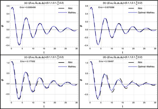
Figure 1. The profile of two-analytical approximations ( |
3. Second approach for analyzing the (un)forced damped PPO
Let us consider the i.v.p.14 ) is assumed to have the following ansatz form18 ) into (17 ), we have
$\begin{eqnarray}\left\{\begin{array}{l}\ddot{\varphi }+2\beta \dot{\varphi }+\phi (t)\sin \varphi =0,\\ \varphi (0)={\varphi }_{0}\,\mathrm{and}\,{\varphi }^{{\prime} }(0)={\dot{\varphi }}_{0}.\end{array}\right.\end{eqnarray}$
The solution to i.v.p. ( $\begin{eqnarray}\varphi (t)=2{\tan }^{-1}u(t).\end{eqnarray}$
Then $\begin{eqnarray}{\mathbb{R}}=\displaystyle \frac{2}{{\left(u{\left(t\right)}^{2}+1\right)}^{2}}{{\mathbb{R}}}_{u},\end{eqnarray}$
with $\begin{eqnarray}{{\mathbb{R}}}_{u}=\left(\begin{array}{c}-2{u}^{{\prime} }{\left(t\right)}^{2}u(t)+2\beta {u}^{{\prime} }(t)u{\left(t\right)}^{2}+{u}^{{\prime\prime} }(t)u{\left(t\right)}^{2}\\ +u{\left(t\right)}^{3}\phi (t)+u(t)\phi (t)+2\beta {u}^{{\prime} }(t)+{u}^{{\prime\prime} }(t)\end{array}\right).\end{eqnarray}$
Now, let the value of u(t) is given by $\begin{eqnarray}u(t)=\exp (-\beta t)({c}_{1}\cos w(t)+{c}_{2}\sin w(t)).\end{eqnarray}$
By substituting equations ( $\begin{eqnarray}{{\mathbb{R}}}_{u}={S}_{1}\cos w(t)+{S}_{2}\sin w(t)+{\rm{h}}.{\rm{o}}.{\rm{t}}.,\end{eqnarray}$
with $\begin{eqnarray*}\begin{array}{rcl}{S}_{1} & = & \left\{\begin{array}{c}{{\rm{e}}}^{-\beta t}\left[{c}_{2}{w}^{{\prime\prime} }(t)-{c}_{1}\left({\beta }^{2}-\phi (t)+{w}^{{\prime} }{\left(t\right)}^{2}\right)\right]\\ -\tfrac{1}{4}\left({c}_{1}^{2}+{c}_{2}^{2}\right){{\rm{e}}}^{-3\beta t}\left[{c}_{1}\left(9{\beta }^{2}-3\phi (t)+5{w}^{{\prime} }{\left(t\right)}^{2}\right)-{c}_{2}(4\beta {w}^{{\prime} }(t)+{w}^{{\prime\prime} }(t))\right]\end{array}\right\},\\ {S}_{2} & = & \left\{\begin{array}{c}-\tfrac{1}{4}\left({c}_{1}^{2}+{c}_{2}^{2}\right){{\rm{e}}}^{-3\beta t}\left[{c}_{2}\left(9{\beta }^{2}-3\phi (t)+5{w}^{{\prime} }{\left(t\right)}^{2}\right)+{c}_{1}(4\beta {w}^{{\prime} }(t)+{w}^{{\prime\prime} }(t))\right]\\ -{{\rm{e}}}^{-\beta t}\left[{c}_{2}\left({\beta }^{2}-\phi (t)+{w}^{{\prime} }{\left(t\right)}^{2}\right)+{c}_{1}{w}^{{\prime\prime} }(t)\right]\end{array}\right\},\end{array}\end{eqnarray*}$
where ‘h.o.t.' indicates the higher-order terms.Equating both S1 and S2 to zero and then eliminating w″(t) from the resulting system to obtain an ode for w(t). Solving the obtained ode gives the value of the frequency-amplitude formulation as follows
$\begin{eqnarray}\begin{array}{l}w(t)={\int }_{0}^{t} \times \sqrt{\displaystyle \frac{4{{\rm{e}}}^{2\beta \tau }\left(\phi (\tau )-{\beta }^{2}\right)+3\left({c}_{1}^{2}+{c}_{2}^{2}\right)\left(\phi (\tau )-3{\beta }^{2}\right)}{4{{\rm{e}}}^{2\beta \tau }+5\left({c}_{1}^{2}+{c}_{2}^{2}\right)}}\, \text{d} \tau ,\end{array}\end{eqnarray}$
where the constants c1 and c2 are found from the ICs: ${c}_{1}=\tan ({\varphi }_{0}/2)$ and c2 is a solution to the following quartic equation $\begin{eqnarray}{W}_{0}+{W}_{1}{c}_{2}^{2}+{W}_{2}{c}_{2}^{4}=0,\end{eqnarray}$
with $\begin{eqnarray*}\begin{array}{l}{W}_{0}=\tfrac{1}{2}\left(9-\cos \left({\varphi }_{0}\right)\right){\sec }^{6}\left(\tfrac{{\varphi }_{0}}{2}\right)\left(\beta \sin \left({\varphi }_{0}\right)+{\dot{\varphi }}_{0}\right){}^{2},\\ {W}_{1}={\sec }^{4}\left(\tfrac{{\varphi }_{0}}{2}\right)\\ \times \ \left[\begin{array}{l}{\beta }^{2}\left(13+8\cos \left({\varphi }_{0}\right)-5\cos \left(2{\varphi }_{0}\right)\right)-\\ 2{\cos }^{2}\left(\tfrac{{\varphi }_{0}}{2}\right)\left(7+\cos \left({\varphi }_{0}\right)\right){\phi }_{0}+5{\dot{\varphi }}_{0}\left(2\beta \sin \left({\varphi }_{0}\right)+{\dot{\varphi }}_{0}\right)\end{array}\right],\\ {W}_{2}=\left(36{\beta }^{2}-12{\phi }_{0}\right){c}_{2}^{4}=0,\end{array}\end{eqnarray*}$
where φ0 = φ(0).For investigating the accuracy of the obtained solution, we analyze this solution numerically using the following data: $\left(\beta ,{\omega }_{0},{Q}_{0},\gamma \right)=\left(0.1,2,0.1,1\right)$ with the ICs: φ0 = 0 and ${\dot{\varphi }}_{0}=0.1$ which lead to15 ) to the i.v.p. (22 ) is compared with RK4 numerical approximation as illustrated in figure 2. Also, the GMRDE Ld is estimated for $\left(\beta ,{\omega }_{0},{Q}_{0},\gamma ,{\varphi }_{0},{\dot{\varphi }}_{0}\right)=\left(0.1,2,0.1,1,0,0.1\right)$ and $\left(\beta ,{\omega }_{0},{Q}_{0},\gamma ,{\varphi }_{0},{\dot{\varphi }}_{0}\right)=\left(0.1,2,0.1,1,\tfrac{\pi }{6},0.1\right)$, respectively
$\begin{eqnarray}\left\{\begin{array}{l}{\varphi }^{{\prime\prime} }+0.2{\varphi }^{{\prime} }+(2-0.1\cos (t))\sin (\varphi )=0,\\ {\varphi }_{0}=0\,\mathrm{and}\,{\dot{\varphi }}_{0}=0.1.\end{array}\right.\end{eqnarray}$
Solution ( $\begin{eqnarray*}{\left.{L}_{{d}}\right|}_{{\varphi }_{0}=0}=\mathop{\max }\limits_{0\leqslant t\leqslant 30}\left|\mathrm{Approx}.\,(15)-\mathrm{RK}4\right|\,=\,0.000427262.\end{eqnarray*}$
and $\begin{eqnarray*}{\left.{L}_{{d}}\right|}_{{\varphi }_{0}=\tfrac{\pi }{6}}=\mathop{\max }\limits_{0\leqslant t\leqslant 30}\left|\mathrm{Approx}.\,(15)-\mathrm{RK}4\right|\,=\,0.00638336.\end{eqnarray*}$
Now, let us consider the forced parametric pendulum $\begin{eqnarray}\left\{\begin{array}{l}{\mathbb{N}}\equiv \ddot{\varphi }+2\beta \dot{\varphi }+\phi (t)\sin \varphi -F\left(t\right)=0,\\ \varphi (0)={\varphi }_{0}\,\mathrm{and}\,{\varphi }^{{\prime} }(0)={\dot{\varphi }}_{0},\end{array}\right.\end{eqnarray}$
where $F\left(t\right)={F}_{0}\cos (\omega t)$.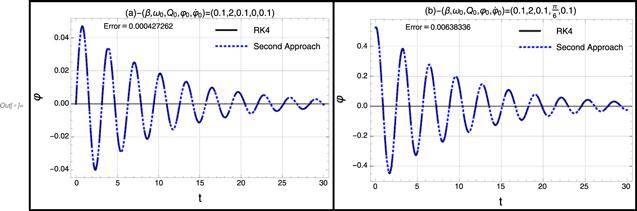
Figure 2. The profile of the approximation ( |
The solution to i.v.p. (23 ) is assumed to have the following ansatz form27 ).
$\begin{eqnarray}\varphi (t)=\theta +{{d}}_{1}\cos \omega t+{{d}}_{2}\sin \omega t,\end{eqnarray}$
where the function θ ≡ θ(t) is a solution to the following unforced pendulum $\begin{eqnarray}\left\{\begin{array}{l}\ddot{\theta }+2\beta \dot{\theta }+\phi (t)\sin \theta =0,\\ \theta (0)={\varphi }_{0}-{{d}}_{1}\,\mathrm{and}\,{\theta }^{{\prime} }(0)={\dot{\varphi }}_{0}-{{d}}_{2}\omega .\end{array}\right.\end{eqnarray}$
For $\sin \varphi \approx \varphi -\tfrac{1}{6}{\varphi }^{3}$, we have $\begin{eqnarray}\begin{array}{rcl}{\mathbb{N}} & \approx & \ddot{\varphi }+2\beta \dot{\varphi }+\left({\omega }_{0}^{2}-{Q}_{0}\cos (\gamma t)\right)\,\left(\varphi -\displaystyle \frac{1}{6}{\varphi }^{3}\right)-F\left(t\right)\\ & = & {X}_{1}\cos (\omega t)+{X}_{2}\sin (\omega t)+{\rm{h}}.{\rm{o}}.{\rm{t}}.\end{array}\end{eqnarray}$
with $\begin{eqnarray*}\begin{array}{rcl}{X}_{1} & = & 2\beta \omega {{d}}_{2}-{F}_{0}-\displaystyle \frac{1}{8}{{d}}_{1}^{3}{\omega }_{0}^{2}+{{d}}_{1}\left(-{\omega }^{2}+{\omega }_{0}^{2}-\displaystyle \frac{1}{8}{{d}}_{2}^{2}{\omega }_{0}^{2}\right)\\ & & +\displaystyle \frac{1}{8}{{d}}_{1}\left(-8+{{d}}_{1}^{2}+{{d}}_{2}^{2}\right){Q}_{0}\cos (\gamma t)\\ & & -\displaystyle \frac{1}{2}{{d}}_{1}\left({\omega }_{0}^{2}-{Q}_{0}\cos (\gamma t)\right)\theta {\left(t\right)}^{2},\end{array}\end{eqnarray*}$
and $\begin{eqnarray*}\begin{array}{rcl}{X}_{2} & = & -2\beta \omega {{d}}_{1}-{\omega }^{2}{{d}}_{2}+{\omega }_{0}^{2}{{d}}_{2}-\displaystyle \frac{1}{8}{\omega }_{0}^{2}{{d}}_{1}^{2}{{d}}_{2}\\ & & -\displaystyle \frac{1}{8}{\omega }_{0}^{2}{{d}}_{2}^{3}+\displaystyle \frac{1}{8}{{d}}_{2}\left({{d}}_{1}^{2}+{{d}}_{2}^{2}-8\right){Q}_{0}\cos (\gamma t)\\ & & -\displaystyle \frac{1}{2}{{d}}_{2}\left({\omega }_{0}^{2}-{Q}_{0}\cos (\gamma t)\right)\theta {\left(t\right)}^{2}.\end{array}\end{eqnarray*}$
We will choose the values of d1 and d2 so that $\begin{eqnarray}\left\{\begin{array}{l}2\beta \omega {{d}}_{2}-{F}_{0}-\displaystyle \frac{1}{8}{{d}}_{1}^{3}{\omega }_{0}^{2}+{{d}}_{1}\left(-{\omega }^{2}+{\omega }_{0}^{2}-\displaystyle \frac{1}{8}{{d}}_{2}^{2}{\omega }_{0}^{2}\right)=0,\\ -2\beta \omega {{d}}_{1}-{\omega }^{2}{{d}}_{2}+{\omega }_{0}^{2}{{d}}_{2}-\displaystyle \frac{1}{8}{\omega }_{0}^{2}{{d}}_{1}^{2}{{d}}_{2}-\displaystyle \frac{1}{8}{\omega }_{0}^{2}{{d}}_{2}^{3}=0.\end{array}\right.\end{eqnarray}$
We choose the least in magnitude real roots to the system (Solution (24 ) for $\left(\beta ,{\omega }_{0},{Q}_{0},\gamma ,{F}_{0},\omega \right)=\left(0.1,2,0.1,1,0.1,0.1\right)$ and different values to $\left({\varphi }_{0},{\dot{\varphi }}_{0}\right)\ $ is introduced in figure 3. Also, the GMRDE Ld is estimated as follows24 ) and the RK4 numerical approximation was observed, as shown in figure 3. Moreover, the obtained approximation (24 ) is characterized by high-accuracy, as is evident from the GMRDE Ld.
$\begin{eqnarray*}{\left.{L}_{{d}}\right|}_{{\varphi }_{0}=0}=\mathop{\max }\limits_{0\leqslant t\leqslant 30}\left|\mathrm{Approx}.\,(24)-\mathrm{RK}4\right|\,=\,0.00135514.\end{eqnarray*}$
and $\begin{eqnarray*}{\left.{L}_{{d}}\right|}_{{\varphi }_{0}=\tfrac{\pi }{6}}=\mathop{\max }\limits_{0\leqslant t\leqslant 30}\left|\mathrm{Approx}.\,(24)-\mathrm{RK}4\right|\,=\,0.014404.\end{eqnarray*}$
The exact match between the obtained approximation (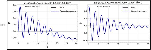
Figure 3. The profile of the approximation ( |
4. He's-FAP for analyzing the (un)damped pendulum oscillator
Let us consider the i.v.p.28 ) reduces to31 ) so that if φ = φ(t) is a solution, then we have33 ) yields
$\begin{eqnarray}\left\{\begin{array}{l}\ddot{\varphi }+2\beta \dot{\varphi }+\phi (t)\sin \varphi =0,\\ \varphi (0)={\varphi }_{0}\,\mathrm{and}\,{\varphi }^{{\prime} }(0)={\dot{\varphi }}_{0}.\end{array}\right.\end{eqnarray}$
For β = 0 and $\sin \varphi \approx \varphi -\tfrac{1}{6}{\varphi }^{3}+\tfrac{1}{120}{\varphi }^{5},$ the i.v.p. ( $\begin{eqnarray}\left\{\begin{array}{l}\ddot{\varphi }+f\left(\varphi \right)=0,\\ \varphi (0)={\varphi }_{0}\,\mathrm{and}\,{\varphi }^{{\prime} }(0)={\dot{\varphi }}_{0},\end{array}\right.\end{eqnarray}$
with $\begin{eqnarray}f\left(\varphi \right)=\phi (t)\left(\varphi -\displaystyle \frac{1}{6}{\varphi }^{3}+\displaystyle \frac{1}{120}{\varphi }^{5}\right).\end{eqnarray}$
He's principle states that [41–46] $\begin{eqnarray}{\omega }^{2}={w}^{{\prime} }{\left(t\right)}^{2}={\left.\displaystyle \frac{f\left(\varphi \right)}{\varphi }\right|}_{\varphi =\tfrac{\sqrt{3}}{2}A}=\phi (t)\left(1-\displaystyle \frac{{A}^{2}}{8}+\displaystyle \frac{3{A}^{4}}{640}\right).\end{eqnarray}$
For the damped case, we can replace A with $A\exp (-\beta t)$ in relation ( $\begin{eqnarray}\varphi (t)=A\exp (-\beta t)\cos (w(t)+B),\end{eqnarray}$
with $\begin{eqnarray}{w}^{{\prime} }{\left(t\right)}^{2}=\phi (t)\left(1-\displaystyle \frac{{A}^{2}}{8}\exp (-2\beta t)+\displaystyle \frac{3{A}^{4}}{640}\exp (-4\beta t)\right),\end{eqnarray}$
and the integration of relation ( $\begin{eqnarray}\begin{array}{l}w(t)={\int }_{0}^{t} \times \ \sqrt{\phi (\tau )\left(1-\displaystyle \frac{{A}^{2}}{8}\exp (-2\beta \tau )+\displaystyle \frac{3{A}^{4}}{640}\exp (-4\beta \tau )\right)} \times \ \text{d} \tau +B.\end{array}\end{eqnarray}$
The constants A and B are found from the ICs.The approximation (32 ) for $\left(\beta ,{\omega }_{0},{Q}_{0},\gamma \right)=\left(0.1,2,0.1,1\right)$ and $\left({\varphi }_{0},{\dot{\varphi }}_{0}\right)=\left(\tfrac{\pi }{6},0.1\right)$, is presented in figure 4. Also, the GMRDE Ld for the approximation (32 ) is estimated as follows
$\begin{eqnarray*}{L}_{{\rm{d}}}=\mathop{\max }\limits_{0\leqslant t\leqslant 30}\left|\mathrm{Approx}.\,(32)-\mathrm{RK}4\right|=0.00631863.\end{eqnarray*}$
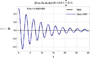
Figure 4. The profile of the approximation ( |
5. He's-HT for analyzing the forced (un)damped PPO
In the beginning, let us consider the forced undamped oscillator
$\begin{eqnarray}\left\{\begin{array}{l}\ddot{\varphi }+\phi \left(t\right)\sin \varphi =F\left(t\right),\\ \varphi (0)={\varphi }_{0}\,\mathrm{and}\,{\varphi }^{{\prime} }(0)={\dot{\varphi }}_{0},\end{array}\right.\end{eqnarray}$
where $F\left(t\right)={F}_{0}\cos ({wt})$.We will replace the i.v.p. (35 ) with the i.v.p.
$\begin{eqnarray}\left\{\begin{array}{l}\ddot{\varphi }+\left({\omega }_{0}^{2}-{Q}_{0}\cos (\gamma t)\right)\left(\varphi -\displaystyle \frac{1}{6}{\varphi }^{3}+\displaystyle \frac{1}{120}{\varphi }^{5}\right)=F\left(t\right),\\ \varphi (0)={\varphi }_{0}\,\mathrm{and}\,{\varphi }^{{\prime} }(0)={\dot{\varphi }}_{0}.\end{array}\right.\end{eqnarray}$
The following homotopy is considered [46–49] $\begin{eqnarray}\begin{array}{l}H(\rho )=\ddot{\varphi }+{\omega }_{0}^{2}\varphi +\rho \left(-{Q}_{0}\cos (\gamma t)\varphi -\displaystyle \frac{1}{6}\phi \left(t\right){\varphi }^{3}\right.\\ \quad \left.+\displaystyle \frac{1}{120}\phi \left(t\right){\varphi }^{5}-F\left(t\right)\right).\end{array}\end{eqnarray}$
Assuming the solution is given by the following ansatz form $\begin{eqnarray}\varphi (t)=A\cos \omega t+\rho u+{\rho }^{2}\,v+\cdots ,\end{eqnarray}$
with $\begin{eqnarray}\omega =\sqrt{{\omega }_{0}^{2}+\rho {\omega }_{1}+{\rho }^{2}{\omega }_{2}\,+\,\cdots },\end{eqnarray}$
where u ≡ u(ωt) and v ≡ v(ωt).Inserting both equations (38 ) and (39 ) into equation (37 ), we final get
$\begin{eqnarray}H(\rho )=\rho {Y}_{1}+{\rho }^{2}{Y}_{2}\,+\cdots ,\end{eqnarray}$
where Y1 and Y2 are defined in appendix (I). Equating to zero the coefficients ${Y}_{{i}}\left({i}=1,2,3,\cdots \right)$ and then solving the resulting ode system, we have $\begin{eqnarray}{\omega }_{1}=\displaystyle \frac{1}{192}{A}^{4}{\omega }_{0}^{2}-\displaystyle \frac{1}{8}{A}^{2}{\omega }_{0}^{2},\end{eqnarray}$
and $\begin{eqnarray}u(\tau )=\displaystyle \frac{1}{{Z}_{9}}\sum _{{i}=1}^{8}{Z}_{{i}},\end{eqnarray}$
where the values of ${Z}_{{i}}\left({i}=1,2,\cdots 9\right)$ are defined in appendix (II).By substituting equation (41 ) into equation (39 ), the following frequency-amplitude formula is obtained38 ) and in frequency-amplitude formula (39 ) or (43 ).
$\begin{eqnarray}\omega ={\omega }_{0}\sqrt{1-\displaystyle \frac{1}{8}{A}^{2}+\displaystyle \frac{1}{192}{A}^{4}}.\end{eqnarray}$
For the damped case, we can replace A with $A\exp (-\beta t)$ solution (The approximation (38 ) for both unforced (F0 = 0) and forced (F0 = 0.1 & w = 0.1) damped PPO is introduced in figure 5 for $\left(\beta ,{\omega }_{0},{Q}_{0},\gamma \right)=\left(0.1,2,0.1,1\right)$ and with different values to $\left({\varphi }_{0},{\dot{\varphi }}_{0}\right)$. Also, the GMRDE Ld for both unforced (F0 = 0) and forced (F0 = 0.1 & w = 0.1) are estimated as follow
$\begin{eqnarray*}\begin{array}{rcl}{\left.{L}_{{\rm{d}}}\right|}_{\left({\varphi }_{0},{F}_{0}\right)=\left(0,0\right)} & = & \mathop{\max }\limits_{0\leqslant t\leqslant 30}\left|\mathrm{Approx}.\,(38)-\mathrm{RK}4\right|\\ & = & 0.00171708,\\ {\left.{L}_{{\rm{d}}}\right|}_{\left({\varphi }_{0},{F}_{0}\right)=\left(0,0.1\right)} & = & \mathop{\max }\limits_{0\leqslant t\leqslant 30}\left|\mathrm{Approx}.\,(38)-\mathrm{RK}4\right|\\ & = & 0.00249545\end{array}\end{eqnarray*}$
and $\begin{eqnarray*}\begin{array}{rcl}{\left.{L}_{{\rm{d}}}\right|}_{\left({\varphi }_{0},{F}_{0}\right)=\left(\tfrac{\pi }{6},0\right)} & = & \mathop{\max }\limits_{0\leqslant t\leqslant 30}\left|\mathrm{Approx}.\,(38)-\mathrm{RK}4\right|\\ & = & 0.0236368,\\ {\left.{L}_{{\rm{d}}}\right|}_{\left({\varphi }_{0},{F}_{0}\right)=\left(\tfrac{\pi }{6},0.1\right)} & = & \mathop{\max }\limits_{0\leqslant t\leqslant 30}\left|\mathrm{Approx}.\,(38)-\mathrm{RK}4\right|\\ & = & 0.022029\end{array}\end{eqnarray*}$
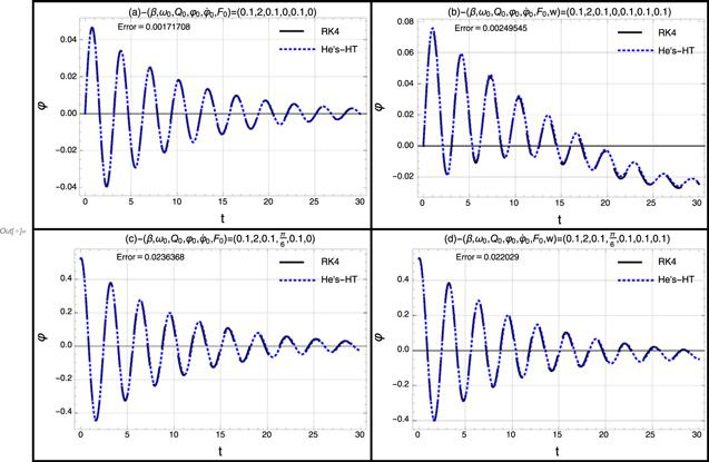
Figure 5. The profile of the approximation ( |
6. The p-solution Method
Now, we proceed for analyzing the following the forced damped i.v.p.44 ) in the form of p- problem is considered45 ) is assumed to be
$\begin{eqnarray}\left\{\begin{array}{l}\ddot{\varphi }+2\beta \dot{\varphi }+\phi (t)\sin \varphi =F\left(t\right),\\ \varphi (0)={\varphi }_{0}\,\mathrm{and}\,{\varphi }^{{\prime} }(0)={\dot{\varphi }}_{0},\end{array}\right.\end{eqnarray}$
for $\sin \varphi \approx \varphi -\tfrac{1}{6}{\varphi }^{3}+\tfrac{1}{120}{\varphi }^{5}$ and $F\left(t\right)={F}_{0}\cos ({wt})$, using the p-solution Method. To do that, the forced damped i.v.p. ( $\begin{eqnarray}\left\{\begin{array}{l}\ddot{\varphi }+{\omega }_{0}^{2}\varphi +p\left(2\beta \dot{\varphi }-{Q}_{0}\cos (\gamma t)\varphi -\displaystyle \frac{1}{6}\phi (t){\varphi }^{3}+\displaystyle \frac{1}{120}\phi (t){\varphi }^{5}-F\left(t\right)\right)=0,\\ \varphi (0)={\varphi }_{0}\,\mathrm{and}\,{\varphi }^{{\prime} }(0)={\dot{\varphi }}_{0}.\end{array}\right.\end{eqnarray}$
The solution of equation ( $\begin{eqnarray}{\varphi }_{p}={\varphi }_{p}(t)=a\cos \left(\psi \right)+\sum _{n=1}^{N}{p}^{n}{u}_{n}(a,\psi )+O({p}^{N+1}),\end{eqnarray}$
where each un ≡ un(a, ψ) is a periodic function of ψ, and the functions $\left(a,\psi \right)\equiv \left(a\left(t\right),\psi \left(t\right)\right)$ are given by $\begin{eqnarray}\displaystyle \frac{{\rm{d}}{a}}{{\rm{d}}{t}}\equiv \dot{a}=\sum _{n=1}^{N}{p}^{n}{A}_{n}(a)+O({p}^{N+1}),\end{eqnarray}$
$\begin{eqnarray}\displaystyle \frac{{\rm{d}}\psi }{{\rm{d}}{t}}\equiv \dot{\psi }={\omega }_{0}+\sum _{n=1}^{N}{p}^{n}{\psi }_{n}(a)+O({p}^{N+1}).\end{eqnarray}$
Based on this technique, the solution of equation (45 ) until p2, reads
$\begin{eqnarray}\varphi (t)=a\cos (\psi )+{{pu}}_{1}(a,\psi )+{p}^{2}{u}_{2}(a,\psi )\,+\,\cdots ,\end{eqnarray}$
where the values of u1(a, ψ) and u2(a, ψ) are defined in appendix (II). The odes for determining the functions $\left(a,\psi \right)$ read $\begin{eqnarray}\dot{a}=-\beta a(t)p+\displaystyle \frac{\beta \phi (t)}{16{\omega }_{0}^{2}}a{\left(t\right)}^{3}\left[\displaystyle \frac{1}{12}a{\left(t\right)}^{2}-1\right]{p}^{2},\end{eqnarray}$
and $\begin{eqnarray}\dot{\psi }={\omega }_{0}+p{\psi }_{1}+{p}^{2}{\psi }_{2},\end{eqnarray}$
with $\begin{eqnarray*}\begin{array}{rcl}{\psi }_{1} & = & \displaystyle \frac{a{\left(t\right)}^{4}\phi (t)\left((5p-8){\omega }_{0}^{2}-9{{pQ}}_{0}\cos (\gamma t)\right)}{3072{\omega }_{0}^{3}}\\ & & -\displaystyle \frac{a{\left(t\right)}^{2}\phi (t)\left({{pQ}}_{0}\cos (\gamma t)+2{\omega }_{0}^{2}\right)}{32{\omega }_{0}^{3}}-\displaystyle \frac{{Q}_{0}\cos (\gamma t)}{2{\omega }_{0}},\end{array}\end{eqnarray*}$
and $\begin{eqnarray*}\begin{array}{rcl}{\psi }_{2} & = & -\displaystyle \frac{{\beta }^{2}}{2{\omega }_{0}}-\displaystyle \frac{{Q}_{0}^{2}{\cos }^{2}(\gamma t)}{8{\omega }_{0}^{3}}+\displaystyle \frac{\phi (t){}^{2}}{9216{\omega }_{0}^{3}}a{\left(t\right)}^{6}\\ & & -\displaystyle \frac{11a{\left(t\right)}^{8}\phi (t){}^{2}}{8847360{\omega }_{0}^{3}}.\end{array}\end{eqnarray*}$
Observe that this method can be applied for any oscillator, conservative, autonomous or not. The results are different from that obtained using He's-HT. On the other hand, He's-HT is hard to apply for a nonconservative oscillators. Even if the application is possible, the results are too large and cumbersome, as we saw in the previous section. Moreover, the solutions obtained using the p-method are simpler. The solution to the original problem is obtained for p = 1.The approximation (49 ) for both unforced (F0 = 0) and forced (F0 = 0 & w = 3) damped PPO is introduced in figure 6 for $\left(\beta ,{\omega }_{0},{Q}_{0},\gamma ,{\dot{\varphi }}_{0}\right)=\left(0.1,2,0.1,1,0.1\right)$ and with different values to $\left({\varphi }_{0},{F}_{0}\right)$. Also, the GMRDE Ld for both unforced (F0 = 0) and forced (F0 = 0.1 & w = 0.1) are estimated as follow
$\begin{eqnarray*}\begin{array}{rcl}{\left.{L}_{{\rm{d}}}\right|}_{\left({\varphi }_{0},{F}_{0}\right)=\left(0,0\right)} & = & \mathop{\max }\limits_{0\leqslant t\leqslant 30}\left|\mathrm{Approx}.\,(49)-\mathrm{RK}4\right|\\ & = & 0.000522143,\\ {\left.{L}_{{\rm{d}}}\right|}_{\left({\varphi }_{0},{F}_{0}\right)=\left(0,0.1\right)} & = & \mathop{\max }\limits_{0\leqslant t\leqslant 30}\left|\mathrm{Approx}.\,(49)-\mathrm{RK}4\right|\\ & = & 0.000780554,\end{array}\end{eqnarray*}$
and $\begin{eqnarray*}\begin{array}{rcl}{\left.{L}_{{\rm{d}}}\right|}_{\left({\varphi }_{0},{F}_{0}\right)=\left(\tfrac{\pi }{6},0\right)} & = & \mathop{\max }\limits_{0\leqslant t\leqslant 30}\left|\mathrm{Approx}.\,(49)-\mathrm{RK}4\right|\\ & = & 0.0059618,\\ {\left.{L}_{{\rm{d}}}\right|}_{\left({\varphi }_{0},{F}_{0}\right)=\left(\tfrac{\pi }{6},0.1\right)} & = & \mathop{\max }\limits_{0\leqslant t\leqslant 30}\left|\mathrm{Approx}.\,(49)-\mathrm{RK}4\right|\\ & = & 0.00629445.\end{array}\end{eqnarray*}$
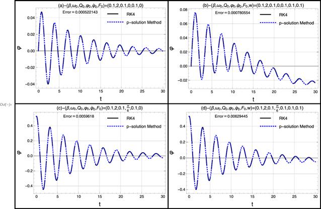
Figure 6. The profile of the approximation ( |
7. Finite different method for analyzing the damped PPO
Suppose we are given the following i.v.p.
$\begin{eqnarray}\left\{\begin{array}{l}\ddot{x}+F(x,\dot{x},t)=0,\\ x(0)={x}_{0}\,\mathrm{and}\,{x}^{{\prime} }(0)={\dot{x}}_{0}.\end{array}\right.\end{eqnarray}$
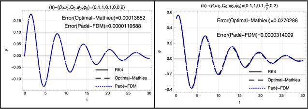
Note here, for simplicity only we put $x\left(t\right)=\varphi (t)\ $ and $F(\varphi ,\dot{\varphi },t)=2\beta \dot{\varphi }+\phi \left(t\right)\sin \left(\varphi \right)$.According to the FDM, we make use the following backward finite difference formulas for the first- and second-derivatives2 ) reads13 ) and both Padé-FDM and RK4 numerical approximations is displayed in figure 7. It is found that the numerical approximation using the Padé-FDM is better than the analytical approximation (13 ). However, in general, both analytical and numerical approximations give highly-accurate and acceptable results. Moreover, the comparison between all proposed techniques at $\left(\beta ,{\omega }_{0},{Q}_{0},\gamma ,{\varphi }_{0},{\dot{\varphi }}_{0}\right)=\left(0.1,1,0.1,1,\pi /6,0.2\right)$ is carried out as follows
$\begin{eqnarray}\begin{array}{rcl}{x}^{{\prime} }\left({t}_{k}\right) & = & \displaystyle \frac{-2{x}_{k-3}+9{x}_{k-2}-18{x}_{k-1}+11{x}_{k}}{6{\rm{\Delta }}t},\\ {x}^{{\prime\prime} }\left({t}_{k}\right) & = & \displaystyle \frac{-{x}_{k-3}+4{x}_{k-2}-5{x}_{k-1}+2{x}_{k}}{{\rm{\Delta }}{t}^{2}}.\end{array}\end{eqnarray}$
In order to obtain suitable values to x1, x2, and x3, we make use the Padé-approximate near t = 0 as follows $\begin{eqnarray}\begin{array}{l}\mathrm{Pad}\acute{{\rm{e}}}(t)={x}_{0}+t\\ \quad \times \left({\dot{x}}_{0}-\displaystyle \frac{3{tF}\left({x}_{0},{\dot{x}}_{0},0\right){}^{2}}{\begin{array}{c}2F\left({x}_{0},{\dot{x}}_{0},0\right)\left({F}^{(\mathrm{0,1,0})}\left({x}_{0},{\dot{x}}_{0},0\right)t+3\right)\\ -2t\left({F}^{(\mathrm{0,0,1})}\left({x}_{0},{\dot{x}}_{0},0\right)+{\dot{x}}_{0}{F}^{(\mathrm{1,0,0})}\left({x}_{0},{\dot{x}}_{0},0\right)\right)\end{array}}\right).\end{array}\end{eqnarray}$
Accordingly, we get $\begin{eqnarray}\left\{\begin{array}{l}{x}_{1}=\mathrm{Pad}\acute{{\rm{e}}}({t}_{1}),\\ {x}_{2}=\mathrm{Pad}\acute{{\rm{e}}}({t}_{2}),\\ {x}_{3}=\mathrm{Pad}\acute{{\rm{e}}}({t}_{3}).\end{array}\right.\end{eqnarray}$
Now, for k = 4, 5, ⋯ , we have $\begin{eqnarray}\begin{array}{l}F\left(z,\displaystyle \frac{-2{x}_{k-3}+9{x}_{k-2}-18{x}_{k-1}+11z}{6{dt}},{t}_{k}\right)\\ \quad +\displaystyle \frac{-{x}_{k-3}+4{x}_{k-2}-5{x}_{k-1}+2z}{{{dt}}^{2}}=0.\end{array}\end{eqnarray}$
This is a transcendental equation for z = xk. We may solve this equation using the Newton–Raphson or other suitable method, taking z = xk−1 as initial value. This way, the FDM gives us the advantage of solving the ode recursively. Thus, the discretization form to the i.v.p. ( $\begin{eqnarray}\begin{array}{l}\displaystyle \frac{-{\varphi }_{k-3}+4{\varphi }_{k-2}-5{\varphi }_{k-1}+2z}{{{d}{t}}^{2}}\\ \quad +2\beta \displaystyle \frac{-2{\varphi }_{k-3}+9{\varphi }_{k-2}-18{\varphi }_{k-1}+11z}{6{d}{t}}\\ \quad +({\omega }_{0}^{2}-{Q}_{0}\cos (\gamma k{\rm{\Delta }}t))\sin \left(z\right)=0,\\ \quad {x}_{0}={\varphi }_{0},{\varphi }_{1}=\mathrm{Pad}\acute{{\rm{e}}}({t}_{1}),{\varphi }_{2}=\mathrm{Pad}\acute{{\rm{e}}}({t}_{2}),\\ \quad \,\mathrm{and}\,{\varphi }_{3}=\mathrm{Pad}\acute{{\rm{e}}}({t}_{3}),z={\varphi }_{k},\\ \quad {t}_{k}=k{\rm{\Delta }}t\,\mathrm{for}\,k=4,5,6,\cdots .\end{array}\end{eqnarray}$
At $\left(\beta ,{\omega }_{0},{Q}_{0},\gamma ,{\dot{\varphi }}_{0}\right)=\left(0.1,1,0.1,1,0.2\right)$ and for different values to φ0 (here φ0 = 0 and φ0 = π/6), the comparison between the analytical approximation ( $\begin{eqnarray*}\begin{array}{rcl}{L}_{{\rm{d}}} & = & \mathop{\max }\limits_{0\leqslant t\leqslant 30}\left|\mathrm{Approxi}.\,(10)-\mathrm{RK}4\right|=0.0285408,\\ {L}_{{\rm{d}}} & = & \mathop{\max }\limits_{0\leqslant t\leqslant 30}\left|\mathrm{Approxi}.\,(13)-\mathrm{RK}4\right|=0.0270288,\\ {L}_{{\rm{d}}} & = & \mathop{\max }\limits_{0\leqslant t\leqslant 30}\left|\mathrm{Approxi}.\,(15)-\mathrm{RK}4\right|=0.0257492,\\ {L}_{{\rm{d}}} & = & \mathop{\max }\limits_{0\leqslant t\leqslant 30}\left|\mathrm{Approxi}.\,(32)-\mathrm{RK}4\right|=0.0293165,\\ {L}_{{\rm{d}}} & = & \mathop{\max }\limits_{0\leqslant t\leqslant 30}\left|\mathrm{Approx}.\,(38)-\mathrm{RK}4\right|=0.0244667,\\ {L}_{{\rm{d}}} & = & \mathop{\max }\limits_{0\leqslant t\leqslant 30}\left|\mathrm{Approx}.\,(49)-\mathrm{RK}4\right|=0.0279174,\\ {L}_{{\rm{d}}} & = & \mathop{\max }\limits_{0\leqslant t\leqslant 30}\left|\mathrm{Pad}\acute{{\rm{e}}}-\mathrm{FDM}-\mathrm{RK}4\right|=0.0000314009.\end{array}\end{eqnarray*}$
Figure 7. The profile of the numerical solutions using both Padé-FDM and RK4 method and the optimal analytical approximation ( |
8. Conclusions
The (un)forced (un)damped PPE have been investigated analytical and numerical using some different approaches. The ansatz method was devoted for deriving some analytical approximations to the damped PPE in the form angular Mathieu functions. Using some suitable assumptions, the obtained analytical approximation has been improved based on two-optimal parameters. In the second approach, the ansatz method was applied for deriving some approximations to the (un)forced damped PPE in the form of trigonometric functions using the ansatz method. In the third approach, He's-FAP was implemented for getting some approximations to the (un)damped PPE. In the forth approach, He's-HT was employed for analyzing the forced (un)damped PPE. In the fifth approach, the p-solution Method was implemented for deriving an approximation to the forced damped PPE. In the final approach, the hybrid Padé-FDM was performed for analyzing the damped PPE. During the numerical simulation, some different cases for small and large angle with the vertical pivot have been discussed. It was found that the accuracy of both first and second formulas for the analytical approximations become identical for small angle, but for large angle the accuracy of second formula becomes better. Furthermore, both analytical and numerical approximations were compared with each other and it turned out that the numerical approximation using Padé-FDM is more accurate than the other approaches. The analytical and numerical techniques that were used in this study can be extended to investigate many nonlinear oscillators.
Acknowledgments
The authors express their gratitude to Princess Nourah bint Abdulrahman University Researchers Supporting Project (Grant No. PNURSP2022R17), Princess Nourah bint Abdulrahman University, Riyadh, Saudi Arabia. Taif University Researchers supporting project number (TURSP-2020/275), Taif University, Taif, Saudi Arabia.
Conflicts of interest
The authors declare that they have no conflicts of interest.
Author contributions
All authors contributed equally and approved the final manuscript.
Appendix
Appendix (I): the coefficients of equation (40 )
$\begin{eqnarray*}{Y}_{1}=\left[\begin{array}{c}-\displaystyle \frac{1}{120}{A}^{5}{Q}_{0}{\cos }^{5}(\tau )\cos \left(\displaystyle \frac{\gamma \tau }{{\omega }_{0}}\right)+\displaystyle \frac{1}{6}{A}^{3}{Q}_{0}{\cos }^{3}(\tau )\cos \left(\displaystyle \frac{\gamma \tau }{{\omega }_{0}}\right)\\ +{\omega }_{0}^{2}\left(\displaystyle \frac{1}{120}{A}^{5}{\cos }^{5}(\tau )-\displaystyle \frac{1}{6}{A}^{3}{\cos }^{3}(\tau )+{u}^{{\prime\prime} }(\tau )+u(\tau )\right)\\ -{{AQ}}_{0}\cos (\tau )\cos \left(\displaystyle \frac{\gamma \tau }{{\omega }_{0}}\right)-A{\omega }_{1}\cos (\tau )-{F}_{0}\cos \left(\displaystyle \frac{\tau w}{{\omega }_{0}}\right)\end{array}\right],\end{eqnarray*}$
and $\begin{eqnarray*}{Y}_{2}=\displaystyle \frac{1}{48{\omega }_{0}^{2}}\left[\begin{array}{c}2{\omega }_{0}^{2}\left(\begin{array}{c}\left(\begin{array}{c}{A}^{2}{\omega }_{0}^{2}{\cos }^{2}(\tau )\left({A}^{2}{\cos }^{2}(\tau )-12\right)-\\ {Q}_{0}\left({A}^{4}{\cos }^{4}(\tau )-12{A}^{2}{\cos }^{2}(\tau )+24\right)\cos \left(\displaystyle \frac{\gamma \tau }{{\omega }_{0}}\right)\end{array}\right)u(\tau )\\ -24A{\omega }_{2}\cos (\tau )+24{\omega }_{0}^{2}\left({v}^{{\prime\prime} }(\tau )+v(\tau )\right)\end{array}\right)\\ +{\omega }_{1}\left(\begin{array}{c}{\omega }_{0}^{2}\left(\begin{array}{c}{A}^{5}(-\tau )\sin (\tau ){\cos }^{4}(\tau )+12{A}^{3}\tau \sin (\tau ){\cos }^{2}(\tau )\\ +24\tau {u}^{(3)}(\tau )+48{u}^{{\prime\prime} }(\tau )+24\tau {u}^{{\prime} }(\tau )\end{array}\right)+\\ {{AQ}}_{0}\tau \sin (\tau )\left({A}^{4}{\cos }^{4}(\tau )-12{A}^{2}{\cos }^{2}(\tau )+24\right)\cos \left(\displaystyle \frac{\gamma \tau }{{\omega }_{0}}\right)\end{array}\right)\\ +24A\tau {\omega }_{1}^{2}\sin (\tau )\end{array}\right],\end{eqnarray*}$
where ω0t = τ.Appendix (II): The values of ${Z}_{{i}}\left({i}=1,2,\cdots ,9\right)$
$\begin{eqnarray*}\begin{array}{rcl}{Z}_{1} & = & 1200Q{{\rm{\Omega }}}^{2}{\cos }^{4}(\tau )\sin (\tau )\\ & & \times \,\sin \left(\displaystyle \frac{{\rm{\Omega }}\tau }{{\omega }_{0}}\right){\omega }_{0}\left({{\rm{\Omega }}}^{2}-4{\omega }_{0}^{2}\right)\left({\omega }_{0}^{2}-{w}^{2}\right){A}^{5},\\ {Z}_{2} & = & {\rm{\Omega }}{\cos }^{5}(\tau )\left({{\rm{\Omega }}}^{2}-4{\omega }_{0}^{2}\right)\left({w}^{2}-{\omega }_{0}^{2}\right)\\ & & \times \left[{{\rm{\Omega }}}^{4}-52{\omega }_{0}^{2}{{\rm{\Omega }}}^{2}+576{\omega }_{0}^{4}-24Q\right.\\ & & \left.\times \,\cos \left(\displaystyle \frac{{\rm{\Omega }}\tau }{{\omega }_{0}}\right)\left({{\rm{\Omega }}}^{2}+24{\omega }_{0}^{2}\right)\right]{A}^{5},\end{array}\end{eqnarray*}$
$\begin{eqnarray*}\begin{array}{rcl}{Z}_{3} & = & 240Q{{\rm{\Omega }}}^{2}{\cos }^{2}(\tau )\sin (\tau )\sin \left(\displaystyle \frac{{\rm{\Omega }}\tau }{{\omega }_{0}}\right){\omega }_{0}\left({w}^{2}-{\omega }_{0}^{2}\right)\\ & & \times \left[\begin{array}{c}-9\left({A}^{2}-16\right){{\rm{\Omega }}}^{2}\\ +16\left(19{A}^{2}-324\right){\omega }_{0}^{2}+20{A}^{2}\cos (2\tau ){\omega }_{0}^{2}\end{array}\right]{A}^{3},\end{array}\end{eqnarray*}$
$\begin{eqnarray*}\begin{array}{rcl}{Z}_{4} & = & 15\left({A}^{2}-16\right){\rm{\Omega }}\cos (3\tau )\left({w}^{2}-{\omega }_{0}^{2}\right)\\ & & \times \left({{\rm{\Omega }}}^{6}-56{\omega }_{0}^{2}{{\rm{\Omega }}}^{4}+784{\omega }_{0}^{4}{{\rm{\Omega }}}^{2}-2304{\omega }_{0}^{6}\right){A}^{3},\end{array}\end{eqnarray*}$
$\begin{eqnarray*}\begin{array}{rcl}{Z}_{5} & = & 5{\rm{\Omega }}{\cos }^{3}(\tau )\left({w}^{2}-{\omega }_{0}^{2}\right)\\ & & \times \left[\begin{array}{c}-{A}^{2}{{\rm{\Omega }}}^{6}+{A}^{2}\cos (2\tau ){{\rm{\Omega }}}^{6}\\ -24Q\cos \left(\displaystyle \frac{{\rm{\Omega }}\tau }{{\omega }_{0}}\right)\left(\begin{array}{c}{A}^{2}\cos (2\tau )\left({{\rm{\Omega }}}^{4}+20{\omega }_{0}^{2}{{\rm{\Omega }}}^{2}-96{\omega }_{0}^{4}\right)\\ -16\left({{\rm{\Omega }}}^{4}+\left(3{A}^{2}-28\right){\omega }_{0}^{2}{{\rm{\Omega }}}^{2}+12\left({A}^{2}-24\right){\omega }_{0}^{4}\right)\end{array}\right)\end{array}\right]{A}^{3},\end{array}\end{eqnarray*}$
$\begin{eqnarray*}\begin{array}{rcl}{Z}_{6} & = & -10\sin (\tau ){\omega }_{0}\left({\omega }_{0}^{2}-{w}^{2}\right)\\ & & \times \left[\begin{array}{c}8{A}^{4}{\rm{\Omega }}{\cos }^{3}(\tau )\sin (\tau ){\omega }_{0}\left(7{{\rm{\Omega }}}^{4}-98{\omega }_{0}^{2}{{\rm{\Omega }}}^{2}+288{\omega }_{0}^{4}\right)\\ -3Q\sin \left(\displaystyle \frac{{\rm{\Omega }}\tau }{{\omega }_{0}}\right)\left(\begin{array}{c}-3{{\rm{\Omega }}}^{4}{A}^{4}+9216{\omega }_{0}^{4}{A}^{4}-412{{\rm{\Omega }}}^{2}{\omega }_{0}^{2}{A}^{4}\\ +{{\rm{\Omega }}}^{2}\cos (4\tau )\left(11{{\rm{\Omega }}}^{2}-4{\omega }_{0}^{2}\right){A}^{4}-192{{\rm{\Omega }}}^{4}{A}^{2}\\ -221184{\omega }_{0}^{4}{A}^{2}+13056{{\rm{\Omega }}}^{2}{\omega }_{0}^{2}{A}^{2}\\ +8{{\rm{\Omega }}}^{2}\cos (2\tau )\left(\left({A}^{2}-24\right){{\rm{\Omega }}}^{2}+4\left(216-13{A}^{2}\right){\omega }_{0}^{2}\right){A}^{2}\\ +3072{{\rm{\Omega }}}^{4}+1769472{\omega }_{0}^{4}-159744{{\rm{\Omega }}}^{2}{\omega }_{0}^{2}\end{array}\right)\end{array}\right]A,\end{array}\end{eqnarray*}$
$\begin{eqnarray*}\begin{array}{l}{Z}_{7}=-\displaystyle \frac{5}{8}{\rm{\Omega }}\cos (\tau )\left({w}^{2}-{\omega }_{0}^{2}\right)\\ \quad \times \left[\begin{array}{c}4\cos (2\tau )\left({{\rm{\Omega }}}^{6}-56{\omega }_{0}^{2}{{\rm{\Omega }}}^{4}+784{\omega }_{0}^{4}{{\rm{\Omega }}}^{2}-2304{\omega }_{0}^{6}\right){A}^{4}\\ -\cos (4\tau )\left({{\rm{\Omega }}}^{6}-56{\omega }_{0}^{2}{{\rm{\Omega }}}^{4}+784{\omega }_{0}^{4}{{\rm{\Omega }}}^{2}-2304{\omega }_{0}^{6}\right){A}^{4}\\ -3\left(\begin{array}{c}{A}^{4}{{\rm{\Omega }}}^{6}-56{A}^{4}{\omega }_{0}^{2}{{\rm{\Omega }}}^{4}-4{A}^{4}Q\cos \left(\tau \left(\displaystyle \frac{{\rm{\Omega }}}{{\omega }_{0}}+4\right)\right){{\rm{\Omega }}}^{4}\\ -32{A}^{4}Q\cos \left(\tau \left(\displaystyle \frac{{\rm{\Omega }}}{{\omega }_{0}}+2\right)\right){{\rm{\Omega }}}^{4}+768{A}^{2}Q\cos \left(\tau \left(\displaystyle \frac{{\rm{\Omega }}}{{\omega }_{0}}+2\right)\right){{\rm{\Omega }}}^{4}\\ -56{A}^{4}Q\cos \left(\displaystyle \frac{{\rm{\Omega }}\tau }{{\omega }_{0}}\right){{\rm{\Omega }}}^{4}+1536{A}^{2}Q\cos \left(\displaystyle \frac{{\rm{\Omega }}\tau }{{\omega }_{0}}\right){{\rm{\Omega }}}^{4}\\ -24576Q\cos \left(\displaystyle \frac{{\rm{\Omega }}\tau }{{\omega }_{0}}\right){{\rm{\Omega }}}^{4}+784{A}^{4}{\omega }_{0}^{4}{{\rm{\Omega }}}^{2}\\ +1664{A}^{4}Q\cos \left(\tau \left(\displaystyle \frac{{\rm{\Omega }}}{{\omega }_{0}}+2\right)\right){\omega }_{0}^{2}{{\rm{\Omega }}}^{2}-21504{A}^{2}Q\cos \left(\tau \left(\displaystyle \frac{{\rm{\Omega }}}{{\omega }_{0}}+2\right)\right){\omega }_{0}^{2}{{\rm{\Omega }}}^{2}\\ -80{A}^{4}Q\cos \left(\tau \left(\displaystyle \frac{{\rm{\Omega }}}{{\omega }_{0}}+4\right)\right){\omega }_{0}^{2}{{\rm{\Omega }}}^{2}+384{A}^{4}Q\cos \left(\tau \left(\displaystyle \frac{{\rm{\Omega }}}{{\omega }_{0}}+4\right)\right){\omega }_{0}^{4}\\ +3488{A}^{4}Q\cos \left(\displaystyle \frac{{\rm{\Omega }}\tau }{{\omega }_{0}}\right){\omega }_{0}^{2}{{\rm{\Omega }}}^{2}-116736{A}^{2}Q\cos \left(\displaystyle \frac{{\rm{\Omega }}\tau }{{\omega }_{0}}\right){\omega }_{0}^{2}{{\rm{\Omega }}}^{2}\\ +1277952Q\cos \left(\displaystyle \frac{{\rm{\Omega }}\tau }{{\omega }_{0}}\right){\omega }_{0}^{2}{{\rm{\Omega }}}^{2}-2304{A}^{4}{\omega }_{0}^{6}\\ +12288{A}^{4}Q\cos \left(\tau \left(\displaystyle \frac{{\rm{\Omega }}}{{\omega }_{0}}+2\right)\right){\omega }_{0}^{4}-221184{A}^{2}Q\cos \left(\tau \left(\displaystyle \frac{{\rm{\Omega }}}{{\omega }_{0}}+2\right)\right){\omega }_{0}^{4}\\ -99072{A}^{4}Q\cos \left(\displaystyle \frac{{\rm{\Omega }}\tau }{{\omega }_{0}}\right){\omega }_{0}^{4}+2211840{A}^{2}Q\cos \left(\displaystyle \frac{{\rm{\Omega }}\tau }{{\omega }_{0}}\right){\omega }_{0}^{4}-14155776Q\cos \left(\displaystyle \frac{{\rm{\Omega }}\tau }{{\omega }_{0}}\right){\omega }_{0}^{4}\\ -4{A}^{4}Q\cos \left(\tau \left(4-\displaystyle \frac{{\rm{\Omega }}}{{\omega }_{0}}\right)\right)\left({{\rm{\Omega }}}^{4}+20{\omega }_{0}^{2}{{\rm{\Omega }}}^{2}-96{\omega }_{0}^{4}\right)\\ -32{A}^{2}Q\cos \left(\tau \left(2-\displaystyle \frac{{\rm{\Omega }}}{{\omega }_{0}}\right)\right)\left(\left({A}^{2}-24\right){{\rm{\Omega }}}^{4}+4\left(168-13{A}^{2}\right){\omega }_{0}^{2}{{\rm{\Omega }}}^{2}-384\left({A}^{2}-18\right){\omega }_{0}^{4}\right)\end{array}\right)\end{array}\right]A\end{array}\end{eqnarray*}$
$\begin{eqnarray*}\begin{array}{rcl}{Z}_{8} & = & -46080\gamma {\rm{\Omega }}\cos \left(\displaystyle \frac{w\tau }{{\omega }_{0}}\right)\left({{\rm{\Omega }}}^{6}-56{\omega }_{0}^{2}{{\rm{\Omega }}}^{4}\right.\\ & & \left.+784{\omega }_{0}^{4}{{\rm{\Omega }}}^{2}-2304{\omega }_{0}^{6}\right),\end{array}\end{eqnarray*}$
$\begin{eqnarray*}\begin{array}{rcl}{Z}_{9} & = & 46080{\rm{\Omega }}\left({w}^{2}-{\omega }_{0}^{2}\right)\left({{\rm{\Omega }}}^{6}-56{\omega }_{0}^{2}{{\rm{\Omega }}}^{4}\right.\\ & & \left.+784{\omega }_{0}^{4}{{\rm{\Omega }}}^{2}-2304{\omega }_{0}^{6}\right).\end{array}\end{eqnarray*}$
Appendix (II): The values of both u1(a, ψ) and u2(a, ψ):
$\begin{eqnarray*}\begin{array}{l}{u}_{1}(a,\psi )=\displaystyle \frac{1}{23040{\omega }_{0}^{2}}\left[{a}^{3}\phi (t)\cos (\psi )\left({a}^{2}(14\cos (2\psi )\right.\right.\\ \quad \left.\left.+\cos (4\psi )-7)-240\cos (2\psi )+120\right)\right]+\displaystyle \frac{F\left(t\right)}{{\omega }_{0}^{2}},\end{array}\end{eqnarray*}$
and $\begin{eqnarray*}\begin{array}{l}{u}_{2}(a,\psi )=\displaystyle \frac{1}{4246732800{\omega }_{0}^{4}}\\ \quad \times \left[\begin{array}{c}{a}^{9}\phi {\left(t\right)}^{2}\left(-5280\cos (3\psi )+160\cos (5\psi )+95\cos (7\psi )+3\cos (9\psi )\right)\\ -1440{a}^{7}\phi {\left(t\right)}^{2}\left(-164\cos (3\psi )+4\cos (5\psi )+\cos (7\psi )\right)\\ +7680{a}^{5}\phi (t)\left[\begin{array}{c}5{\omega }_{0}\left(\begin{array}{c}4\beta (27\sin (3\psi )+\sin (5\psi ))\\ -63{\omega }_{0}\cos (3\psi )+3{\omega }_{0}\cos (5\psi )\end{array}\right)\\ -3{Q}_{0}\cos (\gamma t)\left(\cos (5\psi )-165\cos (3\psi )\right)\end{array}\right]\\ +1474560{a}^{4}\phi (t)F\left(t\right)\left(20\cos (2\psi )+\cos (4\psi )-45\right)\\ -11059200{a}^{3}\phi (t)\left(3\varepsilon {\omega }_{0}\sin (3\psi )+2{Q}_{0}\cos (\gamma t)\cos (3\psi )\right)\\ -353894400{a}^{2}\phi (t)F\left(t\right)\left(\cos (2\psi )-3\right)+4246732800F\left(t\right){Q}_{0}\cos (\gamma t)\end{array}\right].\end{array}\end{eqnarray*}$