


1. Introduction
In the preceding few decades, non-integer order differential equations became an area of interest for researchers owing to their accuracy and applicability in various fields of physics, science, and technology. Many physical, dynamical, biological, and chemical phenomena are represented in a highly effective style by using differential equations having a non-integer rather than integer-order. Being a more accurate approach is the major reason for attracting the attention of researchers. Differential equations having fractional order are suitable for mathematicians, engineers, and physicists. The fractional-order differential equations have a large number of applications in several fields of science and technology, for example, porous media, rheology, optics, electromagnetism, electrochemistry, bio-science, bioengineering, medicine, geology, probability, statistics, etc. The fractional-order differential equations are also applicable in control theory, control of power electrons, tomography, polymer physics, polymer science, and neural networks. Furthermore, it has various applications in the modeling of other phenomena, such as the absorption of drugs in the bloodstream, seepage flow, traffic modeling of fluid dynamics, porous media, image processing, mathematical biology, genetic properties, and nonlinear oscillations resulting from earthquakes. These equations are also used for the calculations of genetically and chemically acquired properties of different materials and phenomena, (see for details [1–7]).
Several physical phenomena are modeled using systems of nonlinear fractional differential equations, which are more accurate for practical applications. Several real phenomena emerging in engineering and science fields can be successfully modeled by developing models which are more accurate than the integer ones [8–10]. The essential quality of fractional-order differential equations is that it yields accurate and stable results. Some of these equations are time-fractional heat equations, time-fractional heat-like equations, time-fractional wave equations, time-fractional telegraphic equations, fractional-order oscillators such as the Van der Pol equation, and so on. These physical equations are performed as linear or nonlinear formulations; and since they have several employments in the field of applied engineering and science, then the analysis of solving such equations is very important. As these equations are generally strenuous to solve, many alternative and powerful methods have been expanded over the last few years. The main advantage of fractional order differential equations is that they produce accurate and stable results. Therefore, these equations represent a significant class of differential equations [11–18].
Fractional calculus (FC) represents a field of mathematics that discusses the non-integer order differentiation and integration and their implications on different physical systems. Generally, the physical situation might predicate its present state and its historical status, which can be confidently modeled by using the technology of FC tools [19, 20]. Accordingly, many analytic methods are derived to deduce exact, explicit, and numerical techniques for nonlinear fractional partial differential equations [21–25]. A lot of fractional-order definitions; while Grunwald–Letnikov, Riemann–Liouville, and Caputo definitions are the majority used in FC research [26].
Schot [27] presented the definition of a jerk as referring to the rate of variation of acceleration. A jerk equation has vast applications in physics and daily life. It has been set to have numerous applications in various areas of science, such as laser physics electrical circuits, acoustics, dynamical processes, and mechanics [28–32]. Jerk is also organized to be governed the flow of a thin-film viscous fluid with a free surface where the surface tension effects play a role typically leading to a third-order equation governing the form of the free surface of the fluid. Jerk also plays a mighty role in the physiological balancing of the human body.
Over the last two decades, there was significant progress in the area of fractional differential equations. Many efforts have been done to the existence of solutions to fractional differential equations [35]. Since the fractional nonlinear operators have a vital role in differential equations, the investigation to find a simple approach alternative to the mathematical hard work is urgent use. One of the several significant operators used to simplify the procedure of nonlinear differential equations is the equivalent linearized method which leads to obtaining the solution easily. A considerable number of valuable research articles can be obtained in the literature regarding this topic, (see for detail [36–38]).
The fractional Van der Pol–Duffing jerk vibration is investigated to give a more perfect description and shed more light on the dynamics of the suggested oscillator. Although the suggested oscillator is simple, it improves complex and noticeable phenomena such as symmetry-breaking bifurcation, bistability, reverses period-doubling, symmetry-restoring crisis, and coexisting attractors [39]. In the present proposal, the linearized equivalent method has been derived or developed to be consistent with solving the fractional jerk oscillator. Afterward, the proposed method is applied to obtain an analytical solution to different cases of the fractional Van der Pol–Duffing jerk oscillator. The technique consists of obtaining the equivalent linearized form with an integer order employing the principle of minimum mean-square error. Then the solution will be available.
2. The methodology
The present section describes the purpose of the fractional jerk oscillator and explains how to find the solution most simply. The simple effective approach is adopted herein utilizing the equivalent linearization technique to solve the fractional Duffing jerk oscillation of the form
$\begin{eqnarray}\dddot{y}(t)=J\left(y,{D}^{\alpha }y,{D}^{\alpha +1}y\right),\,0\lt \alpha \lt 1,\end{eqnarray}$
where ${D}^{\alpha }$ denotes the Riemann–Liouville derivative (in time) of order $\alpha $ and ${\rm{J}}$ stands for a nonlinear polynomial involving the function $y$ and its several fractional-order derivatives. Consider that the above jerk has initial conditions in the form: $\begin{eqnarray}y(0)=A,\,\dot{y}(0)=0,\,\ddot{y}(0)=0.\end{eqnarray}$
The Van der Pol–Duffing jerk oscillator with an integer order is described in the form5 ) or equation (6 ), the result is reduced to equation (3 ). On the other side, when $\varepsilon \to 0$ into equation (5 ), the fractional Duffing jerk oscillator will come. The following second-order Van der Pol–Duffing oscillator is obtained as a limit case of $\alpha \to 0$ into equation (6 ):
$\begin{eqnarray}\dddot{y}+\left(1-\varepsilon {y}^{2}\right)\left(\eta \ddot{y}+\mu \dot{y}\right)+{\omega }_{0}^{3}y+Q{y}^{3}=0,\end{eqnarray}$
where $y,\,\dot{y},\,\ddot{y}$ and $\dddot{y}$ represent a dynamical variable, first-, second-and third-order time derivative, respectively, $\varepsilon $ is a parameter which is used to distinguish the contributions between the model of the Van der Pol–Duffing jerk ($\varepsilon =1$) and the model of the Duffing jerk oscillator. The classical Duffing jerk oscillator can be obtained when $\varepsilon \to 0;$ it becomes $\begin{eqnarray}\dddot{y}+\eta \ddot{y}+\mu \dot{y}+{\omega }_{0}^{3}y+Q{y}^{3}=0.\end{eqnarray}$
The Van der Pol–Duffing jerk oscillator with fractional damped forces is described in the form $\begin{eqnarray}\begin{array}{l}\dddot{y}+\left(1-\varepsilon {y}^{2}\right)\left(\eta {D}^{\alpha +1}y+\mu {D}^{\alpha }y\right)+{\omega }_{0}^{3}y\\ \,+Q{y}^{3}=0;\,0\lt \alpha \lt 1.\end{array}\end{eqnarray}$
The full fractional order of the Van der Pol–Duffing jerk oscillator is assumed to be $\begin{eqnarray}\begin{array}{l}{D}^{\alpha +2}y+\left(1-\varepsilon {y}^{2}\right)\left(\eta {D}^{\alpha +1}y+\mu {D}^{\alpha }y\right)+{\omega }_{0}^{3}y\\ \,+Q{y}^{3}=0;\,0\lt \alpha \lt 1,\end{array}\end{eqnarray}$
where $\eta ,\,\mu ,\,{\omega }_{0}$ and $Q$ are constants. When the order $\alpha $ has been replaced by the unity value in equation ( $\begin{eqnarray}\ddot{y}+\eta \left(1-\varepsilon {y}^{2}\right)\dot{y}+\left({\omega }_{0}^{3}+\mu \right)y+\left(Q-\varepsilon \mu \right){y}^{3}=0.\end{eqnarray}$
The aim is to transform the fractional derivative ${D}^{\alpha }y,\,{D}^{\alpha +1}y$ to the integer derivative $\dot{{\rm{y}}},\ddot{{\rm{y}}},$ respectively, and so on. This aim can be accomplished via the equivalent linearized approach [38]. It is expected that the term ${D}^{\alpha }y$ contributes both to damping and stiffness and the term ${D}^{\alpha +1}y$ is act as the acceleration and the velocity contributions and so on, then there is no loss of generality by replacing the fractional derivatives ${D}^{\alpha }y,\,{D}^{\alpha +1}y$ and ${D}^{\alpha +2}y$ into equation (1 ) by
$\begin{eqnarray}{D}^{\alpha }y\to \left(\displaystyle \frac{{D}^{\alpha }y}{\dot{y}}\right)\dot{y}+\left(\displaystyle \frac{{D}^{\alpha }y}{y}\right)y,\end{eqnarray}$
$\begin{eqnarray}{D}^{\alpha +1}y\to \left(\displaystyle \frac{{D}^{\alpha +1}y}{\ddot{y}}\right)\ddot{y}+\left(\displaystyle \frac{{D}^{\alpha +1}y}{\dot{y}}\right)\dot{y},\end{eqnarray}$
$\begin{eqnarray}{D}^{\alpha +2}y\to \left(\displaystyle \frac{{D}^{\alpha +2}y}{\dddot{y}}\right)\dddot{y}+\left(\displaystyle \frac{{D}^{\alpha +2}y}{\ddot{y}}\right)\ddot{y}.\end{eqnarray}$
It is noted that $\mathop{\mathrm{Lim}\,}\limits_{\alpha \to 1}\,{D}^{\alpha }y=Dy=\dot{y}$ and $\mathop{\mathrm{Lim}\,}\limits_{\alpha \to 0}\,{D}^{\alpha }y=y,$ therefore, when $0\lt \alpha \lt 1$ the fractional derivative can be approximately written as a combination of the damping force and the stiffness force as given by (8). The same reason is done for the case of ${D}^{\alpha +1}y$ and ${{\rm{D}}}^{\alpha +{\rm{2}}}{\rm{y}}.$ These results are due to the application of the equivalent linearized technology.To establish the required formulas for the above relations, the trial displacement function, which should satisfy the initial conditions, is assumed in the following form:1 ), $A$ is the amplitude of the oscillation. Since the trial solution (11) is not exact, then there will be a residual or error remaining. Based on the principle of minimum mean-square error [35], the located displacement point, the velocity point, and the located acceleration point are estimated as given below:
$\begin{eqnarray}\begin{array}{l}{y}_{0}(t)=A\,\cos \,{\rm{\Omega }}t,\,{\dot{y}}_{0}(t)=-A{\rm{\Omega }}\,\sin \,{\rm{\Omega }}t,\\ {\ddot{y}}_{0}(t)=-A{{\rm{\Omega }}}^{2}\,\cos \,{\rm{\Omega }}t,\end{array}\end{eqnarray}$
where ${\rm{\Omega }}$ is assumed to represent the total frequency that controls the fractional nonlinear oscillator equation ( $\begin{eqnarray}{\bar{y}}^{2}=\frac{1}{4T}{\int }_{0}^{T}{y}_{0}^{2}(t){\rm{d}}t=\frac{1}{8}{A}^{2};\,T=\frac{2\pi }{{\rm{\Omega }}},\end{eqnarray}$
$\begin{eqnarray}{\bar{\dot{y}}}^{2}=\frac{1}{4T}{\int }_{0}^{T}{\dot{y}}_{0}^{2}(t){\rm{d}}t=\frac{1}{8}{{\rm{\Omega }}}^{2}{A}^{2},\end{eqnarray}$
$\begin{eqnarray}{\bar{\ddot{y}}}^{2}=\frac{1}{4T}{\int }_{0}^{T}{\ddot{y}}_{0}^{2}(t){\rm{d}}t=\frac{1}{8}{{\rm{\Omega }}}^{4}{A}^{2}.\end{eqnarray}$
Based on the located points mentioned above, Galerkin's formula for the fractional operators will lead to the following equivalents: $\begin{eqnarray}\begin{array}{l}{a}_{eq}\left({\rm{\Omega }}\right)=\frac{1}{\sqrt{2}\,{\rm{\Omega }}T}{\int }_{0}^{T}{\partial }_{A}{\dot{y}}_{0}(t)\,\left(\frac{{D}^{\alpha }{y}_{0}(t)}{\bar{\dot{y}}}\right)\,{\rm{d}}t\\ \,=\,{{\rm{\Omega }}}^{\alpha -1}\,\sin \left(\frac{1}{2}\pi \alpha \right);\,T=\frac{2\pi }{{\rm{\Omega }}},\end{array}\end{eqnarray}$
$\begin{eqnarray}\begin{array}{l}{a}_{eq}\left({\rm{\Omega }}\right)=\frac{1}{\sqrt{2}\,{{\rm{\Omega }}}^{2}T}{\int }_{0}^{T}{\partial }_{A}{\ddot{y}}_{0}(t)\,\left(\frac{{D}^{\alpha +1}{y}_{0}(t)}{\bar{\ddot{y}}}\right)\,{\rm{d}}t\\ \,=\,{{\rm{\Omega }}}^{\alpha -1}\,\sin \left(\frac{1}{2}\pi \alpha \right),\end{array}\end{eqnarray}$
$\begin{eqnarray}\begin{array}{l}{a}_{eq}\left({\rm{\Omega }}\right)=\frac{1}{\sqrt{2}\,{{\rm{\Omega }}}^{3}T}{\int }_{0}^{T}{\partial }_{A}{\dddot{y}}_{0}(t)\,\left(\frac{{D}^{\alpha +2}{y}_{0}(t)}{\bar{\dddot{y}}}\right)\,{\rm{d}}t\\ \,=\,{{\rm{\Omega }}}^{\alpha -1}\,\sin \left(\frac{1}{2}\pi \alpha \right),\end{array}\end{eqnarray}$
$\begin{eqnarray}\begin{array}{l}{b}_{eq}\left({\rm{\Omega }}\right)=\frac{1}{\sqrt{2}\,T}{\int }_{0}^{T}{\partial }_{A}{y}_{0}(t)\,\left(\frac{{D}^{\alpha }{y}_{0}(t)}{\bar{y}}\right)\,{\rm{d}}t\\ \,=\,{{\rm{\Omega }}}^{\alpha }\,\cos \left(\frac{1}{2}\pi \alpha \right),\end{array}\end{eqnarray}$
$\begin{eqnarray}\begin{array}{l}{b}_{eq}\left({\rm{\Omega }}\right)=\frac{1}{\sqrt{2}\,{\rm{\Omega }}T}{\int }_{0}^{T}{\partial }_{A}{\dot{y}}_{0}(t)\,\left(\frac{{D}^{\alpha +1}{y}_{0}(t)}{\bar{\dot{y}}}\right)\,{\rm{d}}t\\ \,=\,{{\rm{\Omega }}}^{\alpha }\,\cos \left(\frac{1}{2}\pi \alpha \right),\end{array}\end{eqnarray}$
$\begin{eqnarray}\begin{array}{l}{b}_{eq}\left({\rm{\Omega }}\right)=\frac{1}{\sqrt{2}\,{{\rm{\Omega }}}^{2}T}{\int }_{0}^{T}{\partial }_{A}{\ddot{y}}_{0}(t)\,\left(\frac{{D}^{\alpha +2}{y}_{0}(t)}{\bar{\ddot{y}}}\right)\,{\rm{d}}t\\ \,=\,{{\rm{\Omega }}}^{\alpha }\,\cos \left(\frac{1}{2}\pi \alpha \right),\end{array}\end{eqnarray}$
where ${\partial }_{A}{\dot{y}}_{0}(t),\,\,{\partial }_{A}{\ddot{y}}_{0}(t)$ and ${\partial }_{A}{\dddot{y}}_{0}(t)$ are the weight residual first, second, and third-order function $\dot{W}(t),$ $\ddot{W}(t)$ and $\dddot{W}(t),$ respectively. The weight function is equal to the function that is used to approximate the solution.According, to the results of (15)–(20) the equivalent to the expansions (8)–(10) becomes1 ) becomes the following linear jerk oscillator:
$\begin{eqnarray}{D}^{\alpha }y={a}_{eq}\left({\rm{\Omega }}\right)\dot{y}+{b}_{eq}\left({\rm{\Omega }}\right)y,\end{eqnarray}$
$\begin{eqnarray}{D}^{\alpha +1}y={a}_{eq}\left({\rm{\Omega }}\right)\ddot{y}+{b}_{eq}\left({\rm{\Omega }}\right)\dot{y},\end{eqnarray}$
$\begin{eqnarray}{D}^{\alpha +2}y={a}_{eq}\left({\rm{\Omega }}\right)\dddot{y}+{b}_{eq}\left({\rm{\Omega }}\right)\ddot{y}.\end{eqnarray}$
Following the recent work [38, 40], the equivalent form of the fractional equation ( $\begin{eqnarray}\dddot{y}(t)=g\left(\ddot{y},\dot{y},y\right),\end{eqnarray}$
where ${\rm{g}}$ refers to a polynomial function with integer derivatives.Firstly, the fractional Duffing jerk oscillator of equation (5 ), where $\varepsilon \to 0,$ will be discussed in the following section:
3. The case of the Duffing jerk oscillator with the fractional damping forces
This section is devoted to the nonlinear Duffing jerk oscillator with fractional damping forces, which is given in the form4 ). Let us postulate that this oscillator is controlled by a total frequency ${\rm{\Omega }}.$ Employing the expressions (21)–(23) into the above equation the equivalent linearized equation corresponding to equation (25 ) may be written in the following approximate form:26 ) is explained in detail in [38, 46–48] and has the form
$\begin{eqnarray}\dddot{y}+\eta {D}^{\alpha +1}y+\mu {D}^{\alpha }y+{\omega }_{0}^{3}y+Q{y}^{3}=0;\,0\lt \alpha \lt 1.\end{eqnarray}$
For the traditional integer order, the above equation is reduced to equation ( $\begin{eqnarray}\begin{array}{l}\dddot{y}+\eta {a}_{eq}({\rm{\Omega }})\ddot{y}+\left(\mu {a}_{eq}({\rm{\Omega }})+\eta {b}_{eq}({\rm{\Omega }})\right)\dot{y}\\ \,+\left({\omega }^{3}+\mu {b}_{eq}({\rm{\Omega }})\right)y=0,\end{array}\end{eqnarray}$
where ${\omega }^{3}$ is the He's frequency formula [41–45] which represents the natural frequency for the equivalent form (19) and which is estimated in [38] to be $\begin{eqnarray}{\omega }^{3}={\left.\frac{{\rm{d}}f(y)}{{\rm{d}}y}\right|}_{y=\frac{1}{2\sqrt{2}}A}={\omega }_{0}^{3}+\frac{3}{8}{A}^{2}Q,\end{eqnarray}$
where $f(y)={\omega }_{0}^{3}y+Q{y}^{3}.$ The exact analytical solution for the linear equation ( $\begin{eqnarray}\begin{array}{l}y(t)=\frac{A}{{\phi }^{2}-2\phi {\rm{\Omega }}+2{{\rm{\Omega }}}^{2}}\left[\left({\phi }^{2}-\phi {\rm{\Omega }}+{{\rm{\Omega }}}^{2}\right){{\rm{e}}}^{-{\rm{\Omega }}t}\right.\\ \,+\left.{\rm{\Omega }}{{\rm{e}}}^{-\phi t}\left(({\rm{\Omega }}-\phi )\cos \,{\rm{\Omega }}t+{\rm{\Omega }}\,\sin \,{\rm{\Omega }}t\right)\right],\end{array}\end{eqnarray}$
where the frequency ${\rm{\Omega }}$ and the parameter $\phi $ are given by $\begin{eqnarray}{{\rm{\Omega }}}^{3}-{\omega }^{3}+\left(\eta {\rm{\Omega }}-\mu \right){\rm{\Omega }}{a}_{eq}-\left(\eta {\rm{\Omega }}+\mu \right){b}_{eq}=0,\end{eqnarray}$
$\begin{eqnarray}\phi =\displaystyle \frac{1}{2{{\rm{\Omega }}}^{2}}\left(\eta {a}_{eq}\,{{\rm{\Omega }}}^{2}-{\omega }^{3}-\mu {b}_{eq}\right).\end{eqnarray}$
Employing the values of ${a}_{eq}$ and ${b}_{eq}$ into (29) and (30) yields $\begin{eqnarray}\begin{array}{l}{{\rm{\Omega }}}^{3}-{\omega }^{3}+{{\rm{\Omega }}}^{\alpha }\left[\left(\eta {\rm{\Omega }}-\mu \right)\sin \left(\displaystyle \frac{1}{2}\pi \alpha \right)\right.\\ \,-\left.\left(\eta {\rm{\Omega }}+\mu \right)\cos \left(\displaystyle \frac{1}{2}\pi \alpha \right)\right]=0,\end{array}\end{eqnarray}$
$\begin{eqnarray}\begin{array}{l}\phi =-\displaystyle \frac{1}{2}{\rm{\Omega }}+\displaystyle \frac{1}{2}{{\rm{\Omega }}}^{\alpha -2}\left[\mu \,\sin \left(\displaystyle \frac{1}{2}\pi \alpha \right)\right.\\ \,+\left.\eta {\rm{\Omega }}\,\cos \left(\displaystyle \frac{1}{2}\pi \alpha \right)\right].\end{array}\end{eqnarray}$
3.1. Solution utilizing the modified HPM coupling with He's frequency formula
To solve the linear fractional jerk oscillator (25) by homotopy perturbation method, the total frequency ${\rm{\Omega }}$ may be introduced into equation (25 ) gives33 ) is written in the form36 ) gives:
$\begin{eqnarray}\left({D}^{3}+{{\rm{\Omega }}}^{3}\right)y=\left({{\rm{\Omega }}}^{3}-{\omega }^{3}\right)y-\eta {D}^{\alpha +1}y-\mu {D}^{\alpha }y,\end{eqnarray}$
where the notation $D$ refers to the ordinary derivative concerned with the variable $t.$ This equation is rearranged in the form $\begin{eqnarray}\begin{array}{l}\left({D}^{2}+{{\rm{\Omega }}}^{2}\right)U={\rm{\Omega }}\dot{U}+{\left(D+{\rm{\Omega }}\right)}^{-1}\left[\left({{\rm{\Omega }}}^{3}-{\omega }^{3}\right)U\right.\\ \,-\left.\eta {D}^{\alpha +1}U-\mu {D}^{\alpha }U\right],\end{array}\end{eqnarray}$
where the following transformation is used: $\begin{eqnarray}\left(D+{\rm{\Omega }}\right)y(t)=U(t).\end{eqnarray}$
The homotopy equation corresponding to equation ( $\begin{eqnarray}\begin{array}{l}\left({D}^{2}+{{\rm{\Omega }}}^{2}\right)U=\rho \left\{{\rm{\Omega }}\dot{U}+{\left(D+{\rm{\Omega }}\right)}^{-1}\right.\\ \times \,\left.\left[\left({{\rm{\Omega }}}^{3}-{\omega }^{3}\right)U-\eta {D}^{\alpha +1}U-\mu {D}^{\alpha }U\right]\right\},\rho \in \left[0,1\right].\end{array}\end{eqnarray}$
Applying the following modified expansion to equation ( $\begin{eqnarray}U(t)={{\rm{e}}}^{-\rho \psi t}\left({U}_{0}(t)+\rho {U}_{1}(t)+\mathrm{...}\right),\end{eqnarray}$
where $\psi $ denotes the total damping factor which is determined through the analysis. Employing (37) into (36), the analysis leads to the following achievements: $\begin{eqnarray}{U}_{0}(t)=A{\rm{\Omega }}\,\cos \,{\rm{\Omega }}t.\end{eqnarray}$
But the function ${U}_{1}(t)$ becomes zero under the following conditions: $\begin{eqnarray}\begin{array}{l}{{\rm{\Omega }}}^{3}-{\omega }^{3}+{{\rm{\Omega }}}^{\alpha }\left[-\left(\eta {\rm{\Omega }}+\mu \right)\cos \left(\tfrac{1}{2}\pi \alpha \right)\right.\\ \left.\,+\,\left(\eta {\rm{\Omega }}-\mu \right)\sin \left(\tfrac{1}{2}\pi \alpha \right)\right]=0,\end{array}\end{eqnarray}$
$\begin{eqnarray}\psi =-\tfrac{1}{2}{\rm{\Omega }}+\tfrac{1}{2}{{\rm{\Omega }}}^{\alpha -2}\left(\eta {\rm{\Omega }}\,\cos \left(\tfrac{1}{2}\pi \alpha \right)+\mu \,\sin \left(\tfrac{1}{2}\pi \alpha \right)\right).\end{eqnarray}$
The comparison between the results formulated by the equivalent linearized method (31) and (32) with the results obtained by homotopy perturbation (39) and (40) shows that there are identical results.According to the above conditions, because of (37) and (38), the analytical solution to equation (34 ) becomes25 ) by the perturbation approach employing (34) into (35) yields39 ), consequently, the approximate solution of the frequency equation can be estimated through the perturbation technique. Therefore, let us postulate that the perturbed form of the frequency equation has the form43 ) is given by
$\begin{eqnarray}U(t)=A{\rm{\Omega }}{{\rm{e}}}^{-\psi t}\,\cos \,{\rm{\Omega }}t.\end{eqnarray}$
To perform the total solution for equation ( $\begin{eqnarray}\begin{array}{l}y(t)=\frac{A}{{\psi }^{2}-2\psi {\rm{\Omega }}+2{{\rm{\Omega }}}^{2}}\left[\left({\psi }^{2}-\psi {\rm{\Omega }}+{{\rm{\Omega }}}^{2}\right){{\rm{e}}}^{-{\rm{\Omega }}t}\right.\\ \,+\left.{\rm{\Omega }}{{\rm{e}}}^{-\psi t}\left(({\rm{\Omega }}-\psi )\cos \,{\rm{\Omega }}t+{\rm{\Omega }}\,\sin \,{\rm{\Omega }}t\right)\right].\end{array}\end{eqnarray}$
It is worthwhile to observe that the fractional power ${\rm{\Omega }}$ is involved in equation ( $\begin{eqnarray}\begin{array}{l}{{\rm{\Omega }}}^{3}-{\omega }^{3}+\delta {{\rm{\Omega }}}^{\alpha }\left[\left(\eta {\rm{\Omega }}-\mu \right)\sin \left(\tfrac{1}{2}\pi \alpha \right)\right.\\ \,-\left.\left(\eta {\rm{\Omega }}+\mu \right)\cos \left(\tfrac{1}{2}\pi \alpha \right)\right]=0,\end{array}\end{eqnarray}$
where $\delta $ is a small parameter represents the perturbation parameter. The approximate solution of equation ( $\begin{eqnarray}{\rm{\Omega }}={{\rm{\Omega }}}_{0}+\delta {{\rm{\Omega }}}_{1},\end{eqnarray}$
where $\begin{eqnarray}{{\rm{\Omega }}}_{0}=\omega ,\end{eqnarray}$
$\begin{eqnarray}\begin{array}{l}{{\rm{\Omega }}}_{1}=-\displaystyle \frac{{{\rm{\Omega }}}_{0}^{\alpha }}{3{{\rm{\Omega }}}_{0}^{2}}\left[\left(\eta {{\rm{\Omega }}}_{0}-\mu \right)\sin \left(\displaystyle \frac{1}{2}\pi \alpha \right)\right.\\ \,-\left.\left(\eta {{\rm{\Omega }}}_{0}+\mu \right)\cos \left(\displaystyle \frac{1}{2}\pi \alpha \right)\right].\end{array}\end{eqnarray}$
Employing (45) and (46) into (44) and letting $\delta \to 1,$ yields the approximate frequency in the form $\begin{eqnarray}\begin{array}{l}{\rm{\Omega }}=\omega -\displaystyle \frac{1}{3}{\omega }^{\alpha -2}\left[\left(\eta \omega -\mu \right)\sin \left(\displaystyle \frac{1}{2}\pi \alpha \right)\right.\\ \,-\left.\left(\eta \omega +\mu \right)\cos \left(\displaystyle \frac{1}{2}\pi \alpha \right)\right].\end{array}\end{eqnarray}$
Secondly, the general case of equation (5 ), where $\varepsilon \gt 0,$ is studied in the next section.
4. The case of the Van der Pol–Duffing jerk oscillator in its fractional-order form
This section deals with the solution of equation (5 ). According to the approach mentioned in the previous section, the equivalent form of equation (5 ) becomes48 ) is the same procedure solution of equation (26 ) as given by (28)–(30). Therefore, the frequency ${\rm{\Omega }}$ and the exponential $\varphi $ will be
$\begin{eqnarray}\dddot{y}+{\eta }_{eq}\ddot{y}+{\mu }_{eq}\dot{y}+{\omega }_{eq}^{3}y=0,\end{eqnarray}$
where the equivalent coefficients ${\eta }_{eq}$ and ${\mu }_{eq}$ are given below: $\begin{eqnarray}\begin{array}{l}{\eta }_{eq}=\mathop{\mathrm{lim}}\limits_{y=\displaystyle \frac{1}{2\sqrt{2}}A}\eta \left(1-\varepsilon {y}^{2}\right){a}_{eq}\left({\rm{\Omega }}\right)\\ \,=\,\eta \left(1-\displaystyle \frac{1}{8}\varepsilon {A}^{2}\right){a}_{eq}\left({\rm{\Omega }}\right),\end{array}\end{eqnarray}$
$\begin{eqnarray}\begin{array}{l}{\mu }_{eq}=\mathop{\mathrm{lim}}\limits_{y=\displaystyle \frac{1}{2\sqrt{2}}A}\left(1-\varepsilon {y}^{2}\right)\left(\mu {a}_{eq}\left({\rm{\Omega }}\right)+\eta {b}_{eq}\left({\rm{\Omega }}\right)\right)\\ \,=\,\left(1-\displaystyle \frac{1}{8}\varepsilon {A}^{2}\right)\left(\mu {a}_{eq}\left({\rm{\Omega }}\right)+\eta {b}_{eq}\left({\rm{\Omega }}\right)\right),\end{array}\end{eqnarray}$
$\begin{eqnarray}\begin{array}{l}{\omega }_{eq}^{3}=\mathop{\mathrm{lim}}\limits_{y=\displaystyle \frac{1}{2\sqrt{2}}A}\displaystyle \frac{\partial }{\partial y}\left({\omega }_{0}^{3}y+Q{y}^{3}+\mu \left(1-\varepsilon {y}^{2}\right){b}_{eq}\left({\rm{\Omega }}\right)y\right)\\ \,=\,{\omega }^{3}+\mu \left(1-\displaystyle \frac{3}{8}\varepsilon {A}^{2}\right){b}_{eq}\left({\rm{\Omega }}\right).\end{array}\end{eqnarray}$
As seen, the procedure of the solution of equation ( $\begin{eqnarray}{{\rm{\Omega }}}^{3}+{\eta }_{eq}{{\rm{\Omega }}}^{2}-{\mu }_{eq}{\rm{\Omega }}-{\omega }_{eq}^{3}=0,\end{eqnarray}$
$\begin{eqnarray}\phi =\displaystyle \frac{1}{2{{\rm{\Omega }}}^{2}}\left({\eta }_{eq}{{\rm{\Omega }}}^{2}-{\omega }_{eq}^{3}\right).\end{eqnarray}$
Employing (49)–(51) into (52) and (53) using (15)–(20) yields $\begin{eqnarray}\begin{array}{l}{{\rm{\Omega }}}^{3}={\omega }^{3}+{{\rm{\Omega }}}^{\alpha }\left[\left(\mu -\eta {\rm{\Omega }}\right)\left(1-\tfrac{1}{8}\varepsilon {A}^{2}\right)\sin \left(\tfrac{1}{2}\pi \alpha \right)\right.\\ \,+\left.\left[\eta {\rm{\Omega }}\left(1-\tfrac{1}{8}\varepsilon {A}^{2}\right)+\mu \left(1-\tfrac{3}{8}\varepsilon {A}^{2}\right)\right]\cos \left(\tfrac{1}{2}\pi \alpha \right)\right],\end{array}\end{eqnarray}$
$\begin{eqnarray}\begin{array}{l}\phi =-\tfrac{1}{2}{\rm{\Omega }}+\tfrac{1}{2}{{\rm{\Omega }}}^{\alpha -2}\left(1-\tfrac{1}{8}\varepsilon {A}^{2}\right)\left[\mu \,\sin \left(\tfrac{1}{2}\pi \alpha \right)\right.\\ \,+\,\left.\eta {\rm{\Omega }}\,\cos \left(\tfrac{1}{2}\pi \alpha \right)\right].\end{array}\end{eqnarray}$
It is noted that as $\varepsilon \to 0$ into (54) and (55) the results reduce to those obtained before in (31) and (32).Thirdly, the case of the full fractional orders form is discussed in the next section:
5. Van der Pol–Duffing jerk in full fractional order
In this section, an important cause of the nonlinear jerk oscillation with the full fractional order is considered in the form60 ) is the fractional frequency-amplitude formula of the full fractional Duffing jerk oscillator.
$\begin{eqnarray}\begin{array}{l}{D}^{\alpha +2}y+\left(1-\varepsilon {y}^{2}\right)\left(\eta {D}^{\alpha +1}y+\mu {D}^{\alpha }y\right)\\ \,+{\omega }_{0}^{3}y+Q{y}^{3}=0;\,0\lt \alpha \lt 1.\end{array}\end{eqnarray}$
Because of the approximate relations (21)–(23) and by utilizing He's frequency formula, the above equation can be sought in the equivalent linearized form as $\begin{eqnarray}{a}_{eq}\dddot{y}+\left({\eta }_{eq}+{b}_{eq}\right)\ddot{y}+{\mu }_{eq}\dot{y}+{\omega }_{eq}^{3}y=0.\end{eqnarray}$
The solution of the linear jerk oscillator (57) is still given by the solution (28) except that the frequency ${\rm{\Omega }}$ and the parameter $\varphi $ have been replaced by $\begin{eqnarray}{{\rm{\Omega }}}^{3}+\left(\displaystyle \frac{{\eta }_{eq}+{b}_{eq}}{{a}_{eq}}\right){{\rm{\Omega }}}^{2}-\displaystyle \frac{{\mu }_{eq}}{{a}_{eq}}{\rm{\Omega }}-\displaystyle \frac{{\omega }_{eq}^{3}}{{a}_{eq}}=0,\end{eqnarray}$
$\begin{eqnarray}\phi =\displaystyle \frac{1}{2{a}_{eq}{{\rm{\Omega }}}^{2}}\left[\left({\eta }_{eq}+{b}_{eq}\right){{\rm{\Omega }}}^{2}-{\omega }_{eq}^{3}\right].\end{eqnarray}$
Insert the values of ${a}_{eq},{b}_{eq},\,{\mu }_{eq},{\eta }_{eq}$ and ${\omega }_{eq}^{3}$ into (58) and (59) yields $\begin{eqnarray}\begin{array}{l}{{\rm{\Omega }}}^{2}=\displaystyle \frac{\eta \left(1-\tfrac{1}{8}\varepsilon {A}^{2}\right)\left(\cos \left(\tfrac{1}{2}\pi \alpha \right)-\,\sin \left(\tfrac{1}{2}\pi \alpha \right)\right)}{\cos \left(\tfrac{1}{2}\pi \alpha \right)+\,\sin \left(\tfrac{1}{2}\pi \alpha \right)}{\rm{\Omega }}\\ \,+\mu \left(1-\tfrac{1}{8}\varepsilon {A}^{2}\right)+\displaystyle \frac{{\omega }^{3}}{{{\rm{\Omega }}}^{\alpha }\left(\sin \left(\tfrac{1}{2}\pi \alpha \right)+\,\cos \left(\tfrac{1}{2}\pi \alpha \right)\right)},\end{array}\end{eqnarray}$
$\begin{eqnarray}\begin{array}{l}\phi =\displaystyle \frac{1}{2{\rm{\Omega }}\,\sin \left(\tfrac{1}{2}\pi \alpha \right)}\left[\left(1-\tfrac{1}{8}\varepsilon {A}^{2}\right)\left(\mu \,\sin \left(\tfrac{1}{2}\pi \alpha \right)\right.\right.\\ \left.\left.\,\,\,+\,\eta {\rm{\Omega }}\,\cos \left(\tfrac{1}{2}\pi \alpha \right)\right)-{{\rm{\Omega }}}^{2}\,\sin \left(\tfrac{1}{2}\pi \alpha \right)\right].\end{array}\end{eqnarray}$
The above equation (6. The equivalent linearized approach to reducing the rank of the jerk oscillator
In this section, the effort in converting the third-order oscillator into an equivalent linear second-order oscillator is interesting. This aim is done for the first time, and the linear equivalence method can be used to reduce the rank of the oscillation. The new approach will be applied to the oscillator given in (4). To illustrate the procedure, equation (4 ) can be arranged in the form63 ) can be solved as a second-order linear equation that has solution arises in the form
$\begin{eqnarray}\left(\displaystyle \frac{\dddot{y}+\eta \ddot{y}}{\ddot{y}}\right)\ddot{y}+\mu \dot{y}+{\omega }_{0}^{3}y+Q{y}^{3}=0.\end{eqnarray}$
As mentioned before the total frequency is selected to be ${\rm{\Omega }}.$ The application of the equivalent linearized technique transforms the above equation to $\begin{eqnarray}{c}_{eq}\ddot{y}+\mu \dot{y}+{\omega }^{3}y=0,\end{eqnarray}$
where ${\omega }^{3}$ is the He's frequency formula as given in (27), while the coefficient ${c}_{eq}$ is estimated as $\begin{eqnarray}\begin{array}{l}{c}_{eq}={\left.\displaystyle \frac{\bar{\dddot{y}}+\eta \bar{\ddot{y}}}{\bar{\ddot{y}}}\right|}_{\begin{array}{l}\bar{\ddot{y}}=\tfrac{1}{2\sqrt{2}}A{{\rm{\Omega }}}^{2},\\ \bar{\dddot{y}}=\tfrac{1}{2\sqrt{2}}A{{\rm{\Omega }}}^{3}\end{array}}=\displaystyle \frac{\tfrac{1}{2\sqrt{2}}A{{\rm{\Omega }}}^{3}+\eta \tfrac{1}{2\sqrt{2}}A{{\rm{\Omega }}}^{2}}{\tfrac{1}{2\sqrt{2}}A{{\rm{\Omega }}}^{2}}\\ \,={\rm{\Omega }}+\eta .\end{array}\end{eqnarray}$
At this stage, equation ( $\begin{eqnarray}y=A{{\rm{e}}}^{-\,\frac{\mu }{2\left({\rm{\Omega }}+\eta \right)}t}\,\cos \,{\rm{\Omega }}t,\end{eqnarray}$
where the frequency ${\rm{\Omega }}$ is given by $\begin{eqnarray}{{\rm{\Omega }}}^{2}=\displaystyle \frac{{\omega }^{3}}{{\rm{\Omega }}+\eta }-\displaystyle \frac{{\mu }^{2}}{4{\left({\rm{\Omega }}+\eta \right)}^{2}}.\end{eqnarray}$
This can be read as $\begin{eqnarray}{{\rm{\Omega }}}^{4}+2\eta {{\rm{\Omega }}}^{3}+{\eta }^{2}{{\rm{\Omega }}}^{2}-{\omega }^{3}{\rm{\Omega }}+\left(\displaystyle \frac{{\mu }^{2}}{4}-{\omega }^{3}\eta \right)=0.\end{eqnarray}$
It is noted that this approach can be used when the coefficient $\eta $ has a larger value than the other parameters of the oscillator (56).
7. Numerical simulation
To have a clear and proper understanding of the properties of the present approach, an illustrative numerical interpolation is done. The comparison of the obtained results in this paper with the numerical solution obtained by the Mathematica software is investigated. The comparison of the quasi-exact solution performed in (28) and the homotopy perturbation solution given by (46) with the numerical solution of the traditional integer-order is studied herein for the case of (i.e. equation (4 )), to illustrate how the equivalent method of the fractional-order is close to the numerically exact solution. Two systems of the numerical values of the given coefficients are considered. One of them produces a growing behavior in the time-history profile, while the other deals with the damping behavior in the time-history description. The comparison of the behavior of the influence of $0\lt \alpha \lt 1$ is between the quasi-exact solution and the solution obtained by HPM.
In figure 1, the numerical solution of equation (4 ), the analytical solution (46) with HPM, and the quasi-exact solution (28) are plotted together, for the case of $\varepsilon =0,$ in one graph for the system of $\eta =\mu =\,{\rm{Q}}=\,{\omega }_{{\rm{0}}}=\,{\rm{A}}=\alpha ={\rm{1}}.$ The numerical solution is plotted by the solid red line; the solution of HPM is drawn by the green dashed line; the quasi-exact solution is displayed by the blue dotted line. This graph shows that there is an excellent agreement among the three different solutions for a system producing a growing behavior. When the system is selected to produce a damping behavior, the same conclusion is found as found in figure 2. The system used to produce the graph in figure 2 is $\eta =\mu ={\rm{1}}\mathrm{.3},\,\varepsilon =0,\,{\rm{Q}}=\,{\omega }_{{\rm{0}}}=\,{\rm{A}}=\alpha ={\rm{1}}.$ The variation in the fractional-order $\alpha $ of the solution (28) has been collected together in figure 3, for the same system given in figure 2. It is observed from the investigation of this graph that the damping behavior for the case $\alpha =1$ still occurs with an increase in its amplitude due to a small decrease in the values of $\alpha .$ Continue in decreasing of $\alpha $ leads to a dramatic change in the damping behavior for the oscillation. In which the growing behavior in the oscillation amplitude is observed.
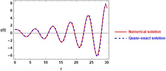
Figure 1. Comparison of the quasi-exact solution (28) (Blue-dashing curve) with the numerical solution of equation ( |

Figure 2. Comparison of the quasi-exact solution (28) with the numerical solution for the system of $\eta =1.2,\mu =1.3,\,\varepsilon =0,\,Q=\,{\omega }_{0}=\,A=\alpha =1.$ |
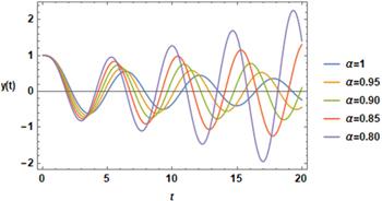
Figure 3. The variation of the parameter $\alpha $ in the profile of the time-history for the same system is considered in figure 2. |
It is worth noting that the forgoing graphs are plotted for the solution (28) in the case of $\varepsilon =0.$ In figures 4–6, the calculations should deal with the case of $\varepsilon \gt 0.$ Figure 4 is plotted using the same system given in the graph of figure 1 except that $\varepsilon =1.$ The comparison between the two graphs of figures 1 and 4 shows that replacing $\varepsilon =0$ by $\varepsilon =1$ leads to an increase in the displacement scale of the growth behavior. Figure 5 is plotted for the same system given in figure 2 but with $\varepsilon =1.$ The comparison between these figures shows a dramatic change occurs. The time-history curve starts as damping behavior and then changes to behave as a growing behavior. The examination of the variation in $\varepsilon $ has been demonstrated in figure 6. In this graph, the solution (28) is plotted for the same system considered in figure 2 with different values $\varepsilon $ to illustrate the influence of $\varepsilon .$ It is worthwhile to note that the system is given in figure 6 starts with damping behavior at $\varepsilon =0.$ It is observed that the amplitude of the damping influence has increased with the increase in $\varepsilon .$ At $\varepsilon =0.5,$ the oscillation becomes with constant amplitude and there is no damping oscillation as shown in figure 7. When $\varepsilon $ becomes $\varepsilon =0.5,$ the oscillation behaves with the same amplitude as a non-damped behavior. After this state of $\varepsilon =0.5,$ the growing behavior in the amplitude of the oscillation will be increased. This behavior should be increased more rapidly for more increase in $\varepsilon .$ This means that there are three cases observed for the variation of $\varepsilon ,$ namely, the damping behavior in the interval of $\varepsilon \in \left[0,\tfrac{1}{2}\right],$ no damped at $\varepsilon =\tfrac{1}{2},$ and growing behavior in the interval of $\varepsilon \in \left[\tfrac{1}{2},0\right].$
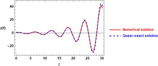
Figure 4. The comparison of two solutions as given in figure 1 except that $\varepsilon =1.$ |
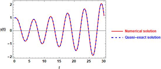
Figure 5. The comparison of the two solutions as given in figure 2 except that $\varepsilon =1.$ |
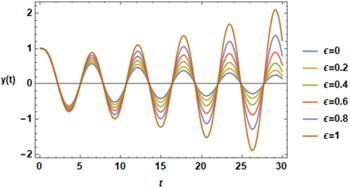
Figure 6. Influence of the variation $\varepsilon $ on the time-history profile for the same system of figure 2. |
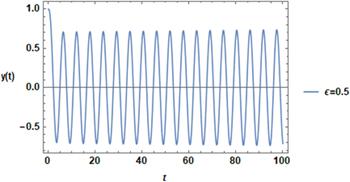
Figure 7. Influence of $\varepsilon =0.5$ on the time-history profile for the same system of figure 2. |
Figure 8 is plotted to examine the solution of equation (56 ) with the variation in the parameter $\alpha .$ The comparison with its numerical solution is done for the case of $\alpha =1$ with $\varepsilon =0.5.$ The remaining parameters are as given in figure 2. This graph shows that the decrease in $\alpha $ has a contribution to the damping influence of the jerk oscillator.
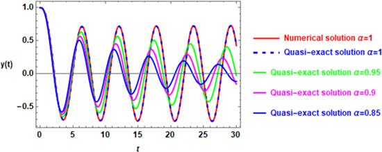
Figure 8. Comparison of the numerical solution of equation ( |
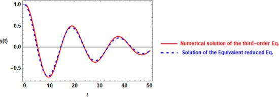
Figure 9 is graphed to clarify the new feature that reduces the rank of the jerk oscillator from the third rank to the second rank. The numerical solution of the original third-order equation (4 ) was compared with the new analytical solution (65) of the second-order equation (63 ), taking into account that $\eta \gg \mu ,{\omega }_{0}^{2}.$ This graph shows that the solution of the reduced equation (63 ) becomes an excellent equivalent to the original equation (4 ).
Figure 9. Comparison of the numerical solution of equation ( |
8. Conclusion
A qualitative study of the efficiency of the simplest analysis of the differential equations based on fractional-order has been considered in the present proposal. The solution of the fractional nonlinear oscillator is obtained by converting it to the linear ordinary differential equation of integer order. This aim is accomplished using the linearized equivalent approach. In the reduced equations, the solution is obtained easily. It has been utilized for the time-fractional Van der Pol–Duffing jerk oscillator. The validation of the proposed technique is emulated with the numerical simulation of the oscillator with integer orders. The obtained solutions might be of huge importance in several areas of applied mathematics in elucidating some physical phenomena. Furthermore, the present approach can be used to reduce the rank of the jerk oscillator under certain conditions. The simplicity of the present approach provides extra advantages for fractional-order solutions.
Competing interests
The author declares that there are no competing interests regarding the publication of the present paper.