We first convert the angular Teukolsky equation under the special condition of τ ≠ 0, s ≠ 0, m = 0 into a confluent Heun differential equation (CHDE) by taking different function transformation and variable substitution. And then according to the characteristics of both CHDE and its analytical solution expressed by a confluent Heun function (CHF), we find two linearly dependent solutions corresponding to the same eigenstate, from which we obtain a precise energy spectrum equation by constructing a Wronskian determinant. After that, we are able to localize the positions of the eigenvalues on the real axis or on the complex plane when τ is a real number, a pure imaginary number, and a complex number, respectively and we notice that the relation between the quantum number l and the spin weight quantum number s satisfies the relation l = ∣s∣+ n, n = 0, 1, 2···. The exact eigenvalues and the corresponding normalized eigenfunctions given by the CHF are obtained with the aid of Maple. The features of the angular probability distribution (APD) and the linearly dependent characteristics of two eigenfunctions corresponding to the same eigenstate are discussed. We find that for a real number τ, the eigenvalue is a real number and the eigenfunction is a real function, and the eigenfunction system is an orthogonal complete system, and the APD is asymmetric in the northern and southern hemispheres. For a pure imaginary number τ, the eigenvalue is still a real number and the eigenfunction is a complex function, but the APD is symmetric in the northern and southern hemispheres. When τ is a complex number, the eigenvalue is a complex number, the eigenfunction is still a complex function, and the APD in the northern and southern hemispheres is also asymmetric. Finally, an approximate expression of complex eigenvalues is obtained when n is greater than ∣s∣.
Chang-Yuan Chen, Xiao-Hua Wang, Yuan You, Dong-Sheng Sun, Fa-Lin Lu, Shi-Hai Dong. Exact solutions to the angular Teukolsky equation with s ≠ 0[J]. Communications in Theoretical Physics, 2022, 74(11): 115001. DOI: 10.1088/1572-9494/ac85d8
1. Introduction
The general form of the angular Teukolsky equation also named as the spin-weighed spheroidal wave equation has played an important role in the study of black holes with the gravitational self-force [1–4], quasi-normal modes [5–8], etc. The equation is given explicitly as [9, 10]
where $x=\,\cos \,\theta ,x\in [-1,+1],\theta \in [0,\pi ],$ and τ = aω. The parameters a and ω represent the angular momentum of per unit mass of the black holes and complex frequency, respectively. The smallest value of the angular quantum number has l = max(∣s∣, ∣m∣), and m = 0, ±1, ±2,··· are the magnetic quantum numbers. The spin weight parameter s of the field is given by s = ±2 for gravitational perturbations, s = ±1 for electromagnetic perturbations, s = ±1/2 for massless neutrino perturbations and s = 0 for scalar perturbations. The eigenfunctions ${\,}_{s}{S}_{lm}(\tau ,\pm 1)$ and eigenvalues ${\,}_{s}{A}_{lm}(\tau )$ are required to be bounded according to the natural boundary conditions. This is a typical Sturm–Liouville boundary problem.
So far the exact analytical solutions to equation (1) have not been obtained except for two particular cases. The first is the case τ = 0 and s = 0. The solutions are well known [11, 12], i.e. its eigenvalues and eigenfunctions are given by ${\,}_{0}{A}_{lm}(0)=l(l+1)$ and ${\,}_{0}{S}_{lm}(0,x)={N}_{lm}{P}_{l}^{m}(x),$ respectively. Here ${P}_{l}^{m}(x)$ are associated Legendre polynomials. The second is the case τ = 0 and s ≠ 0. Its eigenvalues and eigenfunctions are given by
respectively, where ${P}_{n}^{(\alpha ,\beta )}(x)$ are Jacobi polynomials [13, 14]. It can be seen that the angular Teukolsky equation (1) can only exist as an analytical solution under the special condition τ = 0.
There are also two special cases for $\tau \ne 0.$ One is the case s = 0, m ≠ 0 and ${\tau }^{2}=-{c}^{2}$ in equation (1) (the choice of the sign before c2 is different, e.g. a positive sign was used in [15]), then this equation shall become a well-known spheroidal wave equation [16, 17]
This equation has extremely wide applications in many fields such as electromagnetic field theory [17–20], and atomic and molecular physics [21–25]. Up to now, many authors have used different methods to approximately calculate the eigenvalues and the eigenfunctions. The main methods include the expansion of associated Legendre functions [16, 17] and the numerical methods [26–31]. Recently, we have proposed a scheme to construct the Wronskian determinant by finding two linearly dependent solutions with respect to the same eigenstate to obtain accurate eigenvalues and the analytical normalized eigenfunction expressed by a confluent Heun function (CHF) [32, 33]. We find that for a real or pure imaginary τ (c2 = −τ2 is real), the eigenvalues are real. For a complex τ, the eigenvalues are complex. Although the angular probability distribution (APD) has obvious directionality, the northern and southern hemispheres are always symmetric. The advantage of this method is obvious, that is, it not only allows us to obtain accurate eigenvalues (the accuracy of numerical calculation depends on the calculation accuracy of Maple software for CHF and its first derivative) but also can obtain normalized eigenfunction. The analytical wave function makes it possible to discuss properties such as APD. In addition, we have recently obtained the exact solutions of the Stark effect for 3D rigid rotors [34], 2D planar rotors [35], and rigid symmetric top molecules [36] using this method, respectively. The exact solution of the bound state for the Mathieu potential [37] and a kind of hyperbolic potential wells [38] fully demonstrates the merit of this scheme.
In this paper, we mainly study the exact solution of the angular Teukolsky equation for the other special case m = 0, $s\ne 0$ and $\tau \ne 0.$ This will reveal the quantum characteristics of the system under this special condition and provides some ideas for the accurate solution of the general angular Teukolsky equation. When m = 0 but $s\ne 0$ and $\tau \ne 0,$ equation (1) can be simplified as
which is different from equation (2). Thus, its eigenvalues and eigenfunctions have different characteristics from the former (2), which is the main reason why we must study them.
This paper is organized as follows. In section 2 we use different forms of function transformation and variable substitution to convert equation (3) into a confluent Heun differential equation (CHDE), and then according to the characteristics of both the CHDE and its analytical solution expressed by the CHF, two linearly dependent solutions corresponding to the same eigenstate are obtained, and the Wronskian determinant which is constructed by obtained two linearly dependent solutions can be used to obtain the exact eigenvalues. Next, in sections 3–5, we discuss the position of the eigenvalues on the real axis or complex plane when τ is a real number, a pure imaginary number and a complex number, respectively, and determine the relationship between the quantum number l and the spin weight quantum number s, and present the calculation of exact eigenvalues, and the linear dependence of eigenfunctions as well as 2D and 3D graphics of APDs. Finally, we summarize the conclusions in section 6.
2. Construction of the Wronskian determinant
Considering the behaviors of the wave function S(x) with the natural boundary conditions at $x\to \pm 1,$ i.e. zero or finite, we take it as the following form
Particularly, one has ${\rm{HeunC}}\,(\alpha ,\beta ,\gamma ,\delta ,\eta ,0)=1.$ The coefficients ${\upsilon }_{n}$ satisfy a three-term recurrence relation ${A}_{n}{\upsilon }_{n}={B}_{n}{\upsilon }_{n-1}+{C}_{n}{\upsilon }_{n-2}$ with ${\upsilon }_{-1}=0,\,{\upsilon }_{0}=1.$ Generally speaking, to make the CHF ${\rm{HeunC}}(\alpha ,\beta ,\gamma ,\delta ,\eta ,z)$ truncated to an N-term polynomial [39–45], then the determinant constructed from this recurrence relation must satisfy the following two constraints:
However, it is known from equation (7) that the second constraint cannot be satisfied. Thus, we may only obtain a convergent solution of equation (3) at the north pole $(\theta =0\,,\,x=1,\,z=0)$
If we further choose another new variable in equation (5) $z^{\prime} =1-z=(1+x)/2\,,$ $(-1\leqslant x\leqslant 1,\,0\leqslant z^{\prime} \leqslant 1),$ then equation (5) can also be rearranged to the following CHDE
which still doesn’t satisfy the second constraint given in equation (10). Therefore, the solution of equation (3) at the south pole $(\theta =\pi ,\,x=-1,\,z^{\prime} =0)$ is given by
As shown above, both equations (11) and (17) are two solutions of equation (3). Therefore, for the same eigenstate, they only have different mathematical expressions. For a correct and same eigenvalue ${}_{0}A_{l0},$ so they must be linearly dependent within the interval $x\in (-1,+1)$ [46–48]. For two non-zero constants C1 and C2, the solution of equation (3) can be written as the form. Substitutions of equations (11) and (17) into this leads to ${C}_{1}H(1)+{C}_{2}H(2)=0,$ and its first derivative ${C}_{1}H^{\prime} (1)+{C}_{2}H^{\prime} (2)=0.$ As a result, we are able to construct the Wronskian determinant as follows:
Here the function ‘HeunCPrime’ which is defined in Maple denotes the first derivative of the HeunC with respect to the variable z. For convenience, we take $x=0$ in equation (20) to calculate the eigenvalues since they are linearly dependent on the whole interval $x\in (-1,+1).$
It can be seen from formula (20) that the original formula remains unchanged for $\tau =-\tau ,$ so we have
Since equations (22) and (3) must satisfy the same boundary conditions, and the variable x has a symmetric interval, except for the wave function satisfying the relation ${}_{-s}S_{l\,0}(\tau ,x)\,={}_{s}S_{l\,0}(\tau ,-x)$ (ignoring the normalization constant), the eigenvalues must also satisfy the relation ${}_{-s}A_{l\,0}(\tau )\,-2s={}_{s}A_{l\,0}(\tau ),$ i.e.
is a Hermite operator [46–48]. Therefore, its eigenvalues ${}_{s}A_{l0}({\tau }_{R})$ must be real, and its eigenfunctions possessing different eigenvalues are orthogonal to each other. The eigenfunction is made of an orthonormal complete system. From (11), (12), (17) and (18), we know that the functions are all real functions. From equation (20), we define the following functions
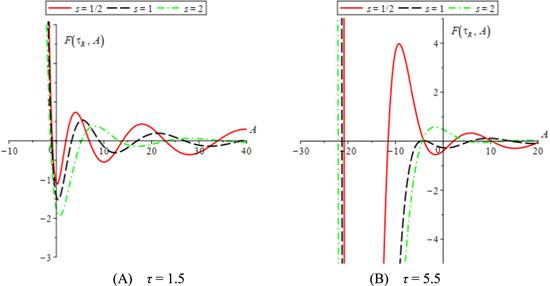
When ${\tau }_{R}$ takes a real number, it represents the change of the function $F({\tau }_{R},A)$ with A, and its intersection with the horizontal axis A determines the corresponding real eigenvalue ${}_{s}A_{l0}({\tau }_{R}).$ As an illustration, figure 1 plots the variation of the function $F({\tau }_{R},A)$ for ${\tau }_{R}$ = 1.5, 5.5 and s = 1/2, 1, 2, respectively. In [33], for the special case s = 0, $m\ne 0$ and $\tau \ne 0,$ we do function substitution $S(x)={(1-{x}^{2})}^{| m| /2}\exp ({\rm{i}}\,c\,x)F(x),$ and get such a relation $l=| m| +n=0,1,2,\mathrm{..}..$ For formula (3), we are now doing the substitution of formula (4), so the generalized angular quantum number l and spin weight quantum number s should satisfy the following equations.
Figure 1. The graphics of F(τ, A) for real numbers τ = 1.5 and 5.5.
For example, the first intersection of each curve with the horizontal axis in figure 1 corresponds to n = 0, the angular quantum number l = ∣s∣, the next one corresponds to $n=1,$ and the angular quantum number is l = ∣s∣+1, and so on (the same below). Here n denotes the number of nodes of the eigenfunction. The exact eigenvalues ${}_{s}A_{l0}({\tau }_{R})$ corresponding to different parameter values can be obtained under a given precision by using Maple software to calculate equation (20). Table 1 lists some results. Note that the values of ±τ and ±s are completely in line with equations (21) and (23), so table 1 only lists the cases where ${\tau }_{R}$ and s take positive values. It is shown from figure 1 and table 1 that when τ = $\pm \,{\tau }_{R}$ is a real number, ${\tau }^{2}={(\pm \,{\tau }_{R})}^{2}\gt 0.$ When τ = 1.5, only the eigenvalue of the ground state n = 0 is less than zero. When τ = 5.5, there exist three states (n = 0, 1, 2) for the cases s = 1/2 and 1 whose eigenvalues are less than zero.
Table 1. The real eigenvalues A for real numbers τ.
s
n
l
τ = 1.5
τ = 5.5
1/2
0
1/2
−0.85180799
−20.79276040
1
3/2
1.99051707
−11.55645908
2
5/2
6.92406087
−4.01977612
3
7/2
13.90248143
2.18912084
1
0
1
−1.00012153
−21.24999757
1
2
3.20141897
−4.87463499
2
3
9.03294081
−3.46818835
3
4
16.97389740
5.78104186
2
0
2
−1.24608944
−22.08176257
1
3
5.28086662
−4.39436169
2
4
13.19908483
5.26662438
3
5
23.11603321
12.64369217
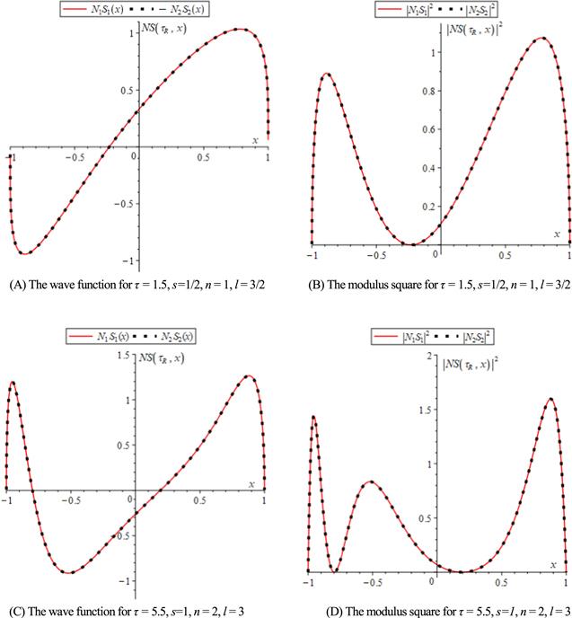
Now, let us study the linear dependence between S(1) and S(2). For this purpose, we substitute the obtained eigenvalues into equations (11) and (17) and then obtain the normalized wave function by performing a normalization operation denoted as ${N}_{1}{S}_{1}({\tau }_{R},x)$ and ${N}_{2}{S}_{2}({\tau }_{R},x).$ We find they satisfy the following relation
where N1 and N2 are two normalization constants. In figure 2 we plot the normalized waves functions of N1S1(${\tau }_{R},$ x), N2S2(${\tau }_{R},$ x) and their modulus squares for ${\tau }_{R}$ = 1.5, $s=1/2,$ n = 1, l = 3/2 and ${\tau }_{R}$ = 5.5, s = 1, n = 2, l = 3, respectively. It can be seen that the two eigenfunctions with respect to the same eigenstate satisfy equation (27), so they are linearly dependent. In addition, we can also see from figure 2 that for a certain state (l, s), the number of nodes of the real eigenfunction is equal to the quantum number n given in equation (26). It can be seen from (21) and (23) that the eigenvalues remain unchanged for $\tau \to -\tau $ and the eigenvalues increase by 2 s in the vase of $s\to -s,$ so how do the eigenfunctions change when these two parameters change? Considering equation (3), we can draw the following conclusions under the condition that τ is a real number: (1) when ${\tau }_{R}\to -{\tau }_{R},$ the eigenvalue remains unchanged, but the first-order term $2{\tau }_{R}sx$ in equation (3) changes sign. Although the variable x has a symmetric interval, the eigenfunction still needs to be changed; (2) when $s\to -s,$ the eigenvalue is increased by 2 s, the first-order term $2{\tau }_{R}sx$ changes sign, so the change of the wave function is the same as the result in case 1); (3) when ${\tau }_{R}\to -{\tau }_{R}$ and $s\to -s,$ the eigenvalue should increase by 2 s, but the first-order term 2τRsx remains unchanged, so the wave function does not change.
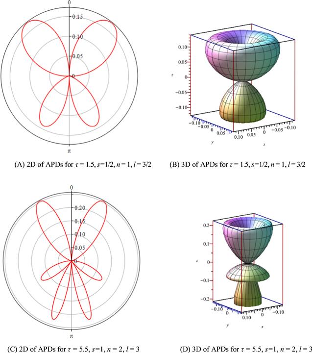
where $\theta \in [0,\pi ].$ As an example, we plot in figure 3 the 2D and 3D graphics of the APDs for τ = 1.5, s = 1/2, n = 1, l = 3/2 and τ = 5.5, s = 1, n = 2, l = 3, respectively. It can be seen that when τ is a real number, a notable feature of the APD not only has obvious directionality but also is asymmetric in the northern and southern hemispheres. Such a phenomenon is obvious, because there is a first-order term $2{\tau }_{R}sx$ in equation (3), and the variation range of x is in the symmetric interval, so the wave function is unequal in the symmetric interval, the modulus square of the wave function is not an even function anymore. This results in the asymmetric APDs in the northern and southern hemispheres.
Figure 3. The plots of APDs in 2D and 3D for the real number τ.
4. Imaginary number τ cases
When $\tau =\pm \,{\rm{i}}\,{\tau }_{I}$ is a pure imaginary number, the operator of boundary value problem for Sturm–Liouville corresponding to equation (3)
is a non-Hermite operator [46–48]. It is easy to show that ${L}_{+}(+{\rm{i}}{\tau }_{I})={\left({L}_{-}(-{\rm{i}}{\tau }_{I})\right)}^{\ast }$ and ${L}_{-}(-{\rm{i}}\,{\tau }_{I})={\left({L}_{+}\,(+{\rm{i}}\,{\tau }_{I})\right)}^{* }.$ This implies that ${}_{s}A_{l0}\,(-{\rm{i}}\,{\tau }_{I})={\left({}_{{\rm{s}}}A_{l0}(+{\rm{i}}\,{\tau }_{I})\right)}^{* }$ and ${}_{s}S_{l0}\left(-{\rm{i}}{\tau }_{I}\right)\,={\left({}_{s}S_{l0}\left(+{\rm{i}}{\tau }_{I}\right)\right)}^{* }$. On the other hand, it can be seen from equation (21) that ${}_{s}A_{l0}(-{\rm{i}}\,{\tau }_{I})={}_{s}A_{l0}(+{\rm{i}}\,{\tau }_{I}),$ so the eigenvalues can only take real values, i.e. ${}_{s}A_{lm}(+{\rm{i}}\,{\tau }_{I})\,={\left({}_{s}A_{lm}(+{\rm{i}}\,{\tau }_{I})\right)}^{* }.$ The eigenfunction is a complex function, and the eigenfunction cannot constitute an orthonormal complete system. According to (20), we can define the following function
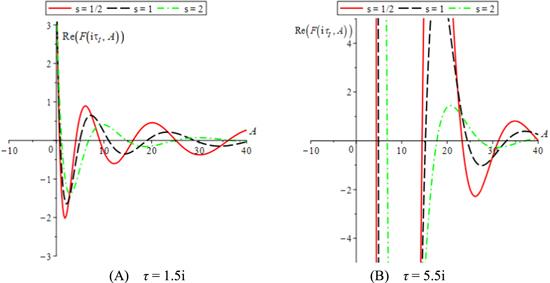
Its intersection with the real A axis determines the real eigenvalue ${}_{s}A_{l0}\,({\rm{i}}\,{\tau }_{I}).$ Figure 4 shows the intersection of the function $\mathrm{Re}(F({\rm{i}}\,{\tau }_{I},A))$ with the real axis A for τ = 1.5i, 5.5i and s = 1/2, 1, 2, respectively. According to the discussion in the previous section, the first intersection of the function $\mathrm{Re}(F({\rm{i}}\,{\tau }_{I},A))$ with the real axis A corresponds to n = 0, the angular quantum number l = ∣s∣, the next corresponds to n = 1, the angular quantum number is l = ∣s∣+1, and so on. The real eigenvalues corresponding to different parameter values can be obtained under a given precision by using Maple software to calculate equation (20). The corresponding calculation results of ${}_{s}A_{l0}\,({\rm{i}}\,{\tau }_{I})$ are listed in table 2. Note that the calculation of the real eigenvalues is exactly the same for the case $\tau =\pm \,{\rm{i}}\,{\tau }_{I},$ and the calculation results of the values of the ±s also completely satisfy formula (23), so table 2 lists the cases where τ is a positive pure imaginary number and s is a positive value. It is found from figure 4 and table 2 that when $\tau =\pm \,{\rm{i}}\,{\tau }_{I}$ is a pure imaginary number, ${\tau }^{2}={(\pm \,{\rm{i}}{\tau }_{I})}^{2}\lt 0,$ the corresponding eigenvalues are greater than zero. This is totally different from the case of real τ whose eigenvalues are also less than zero.
Figure 4. The graphics of F(τ, A) for pure imaginary numbers τ = 1.5i and 5.5i.
Table 2. The real eigenvalues A for pure imaginary numbers τ.
s
n
l
τ = 1.5i
τ = 5.5i
1/2
0
1/2
0.66599153
4.51481928
1
3/2
4.07378564
14.48590438
2
5/2
9.10888852
23.27525125
3
7/2
16.11663584
31.26533349
1
0
1
0.80392011
4.88747469
1
2
4.90970402
15.21854693
2
3
10.98505255
24.41370567
3
4
19.03684060
33.02753668
2
0
2
1.10471291
6.83332976
1
3
6.78647732
17.72154456
2
4
14.82426420
27.26648959
3
5
24.89315062
37.12079162
When $\tau =\pm \,{\rm{i}}\,{\tau }_{I}$ is a pure imaginary number, we know S(1) and S(2) are all complex functions and find they satisfy the following linear dependence relation
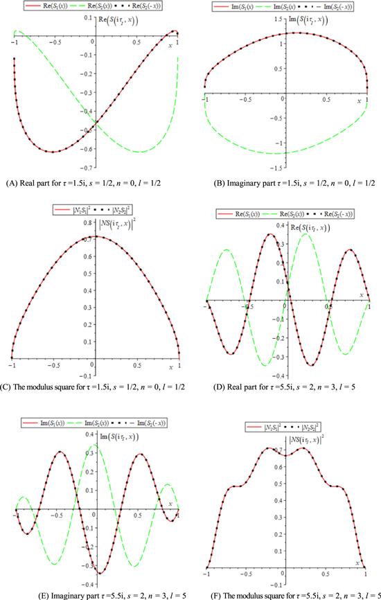
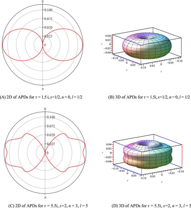
It can be seen from the above formulae that the real parts of S(1) and S(2) are symmetric to the vertical axis, and the imaginary parts of S(1) and S(2) are symmetric to the origin, so their modulus squares is an even function. Figure 5 displays the real and imaginary parts and modulus squares of S(1) and S(2) for τ = 1.5i, s = 1/2, n = 0, l = 1/2 and τ = 5.5i, s = 2, n = 3, l = 5, respectively. It can be seen from figure 5 that when τ is a pure imaginary number, for a certain eigenstate (l, s), the number of nodes of the real and imaginary parts of the eigenfunction will not be equal to n given in equation (26). Figure 6 shows APDs in 2D and 3D for τ = 1.5i, s = 1/2, n = 0, l = 1/2 and τ = 5.5i, s = 2, n = 3, l = 5. It can be seen that when τ is a pure imaginary number, the APD is characterized by obvious directionality, but the northern and southern hemispheres are always symmetric.
Figure 6. The plots of APDs in 2D and 3D for the pure imaginary number τ.
5. Complex number τ cases
When $\tau ={\tau }_{R}+{\rm{i}}{\tau }_{I}$ is a complex number, the operator of boundary value problem for Sturm–Liouville corresponding to equation (3)
is a non-Hermite operator [46–48]. It is easy to show that ${[L({\tau }_{R}+{\rm{i}}\,{\tau }_{I})]}^{* }=[L({\tau }_{R}-{\rm{i}}\,{\tau }_{I})]$ and ${[L({\tau }_{R}-\,{\rm{i}}\,{\tau }_{I})]}^{* }\,=[L({\tau }_{R}+{\rm{i}}\,{\tau }_{I})].$ Therefore, the eigenvalues are complex conjugates to each other, that is,
It can be seen that as long as we calculate the value of ${}_{s}A_{l\,0}({\tau }_{R}+{\rm{i}}{\tau }_{I}),$ the eigenvalues of three cases $\tau ={\tau }_{R}\,-{\rm{i}}\,{\tau }_{I}\,,\,-{\tau }_{R}-{\rm{i}}\,{\tau }_{I}\,,\,-{\tau }_{R}+{\rm{i}}\,{\tau }_{I}$ can be obtained by formulas (33)—(35). The eigenfunctions are also complex conjugates to each other, that is,
However, the eigenfunction cannot make of an orthonormal complete system.
It can be known from (11), (12), (17) and (18) that the functions S(1), S(2), H(1), H(2) are all complex functions. Based on (19) we are able to plot the following two functions in the complex A plane,
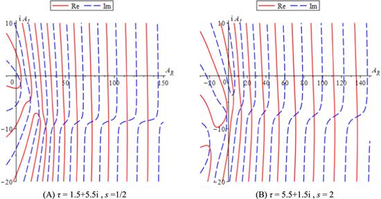
The coordinates of their intersections on the complex A plane determine the real and imaginary parts of the corresponding eigenvalues ${}_{s}A_{\,l\,0}({\tau }_{R}+\,{\rm{i}}{\tau }_{I}).$ For example, figure 7 illustrates the graphs of the two implicit function curves determined by equations (37a) and (37b) when τ = 1.5 + 5.5i, s = 1/2 and τ = 5.5 + 1.5i, s = 2, respectively. According to the previous discussion, the first intersection of the two curves of the real and imaginary parts in each figure corresponds to n = 0, the angular quantum number l = ∣s∣, the next corresponds to n = 1, and the angular quantum number is l = ∣s∣ + 1 and so on. The following two points can be seen in figure 7: (1) when $\tau ={\tau }_{R}+{\rm{i}}{\tau }_{I},$ the sign of the imaginary part of the complex eigenvalue is always opposite to the sign of the imaginary part of τ; (2) when n is greater than ∣s∣, the imaginary part of the eigenvalue becomes more and more approaching a fixed value $-\,{\rm{i}}{\tau }_{R}{\tau }_{I}.$ Table 3 lists the calculation results of the eigenvalues ${}_{s}A_{\,l\,0}({\tau }_{R}+\,{\rm{i}}{\tau }_{I})$ calculated by using Maple software. Note that when $\tau =\pm {\tau }_{R}\pm {\rm{i}}{\tau }_{I},$ the result of the eigenvalue conforms to equations (33)–(35), and the result of ±s is also determined by equation (23), so table 3 lists ${\tau }_{R},$ ${\tau }_{I}$ and s are both positive.
Table 3. The complex eigenvalues A for complex numbers τ.
τ = 1.5 + 5.5i
τ = 5.5 + 1.5i
s
n
l
AR
iAI
AR
iAI
1/2
0
1/2
4.51311795
−1.49530341
−18.53792066
−13.48673615
1
3/2
14.47740752
−4.49621281
−9.24807215
−10.39073413
2
5/2
23.13841449
−7.52454735
−1.38581889
−6.52228221
3
7/2
30.13909324
−9.50354265
1.94788926
−5.39576592
1
0
1
4.88719862
−1.47271049
−18.99999885
−13.49999750
1
2
15.24605752
−4.41091299
−2.33229387
−5.96075080
2
3
24.33699058
−7.60060044
−1.74455881
−7.99839369
3
4
31.60151296
−9.02654552
5.35181170
−5.44954108
2
0
2
6.92203148
−1.64381971
−19.84925208
−13.55110724
1
3
18.01688550
−4.82714578
−2.18529913
−7.43228253
2
4
26.74636804
−8.35589340
5.35924503
−3.46511428
3
5
35.43849104
−7.88790136
13.45754841
−5.96652692
Now, let us study the linear dependence between S(1) and S(2) when τ is a complex function. For this purpose, we substitute the obtained eigenvalues into equations (11) and (17) and then after the normalization operation, the normalized wave function is obtained denoted as ${N}_{1}{S}_{1}(\tau ,\,x)$ and ${N}_{2}{S}_{2}(\tau ,\,x),$ respectively. The linear dependence between S(1) and S(2) requires that two constants that are not equal to zero allow us to get one function of them, say S(2) from another one S(1). That is to say if two constants CR and CI satisfy
Since the linear dependence is in the interval $x\in (a,b),$ the expansion coefficient can be calculated by taking arbitrary value ${x}_{0}$ within this interval
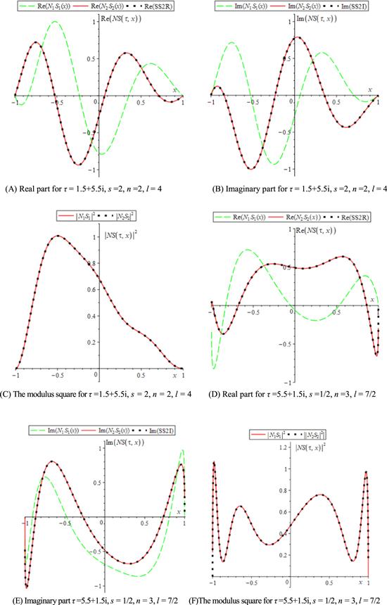
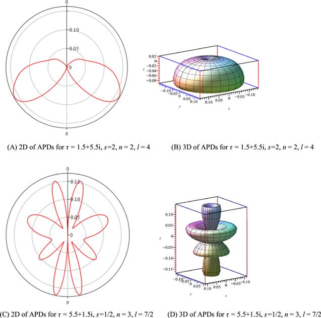
It is known from the fact ${\left|{N}_{2}{S}_{2}(\tau ,\,x)\right|}^{2}={\left|{N}_{1}{S}_{1}(\tau ,\,x)\right|}^{2}$ that ${C}_{R}^{2}+{C}_{I}^{2}=1.$ In figure 8, we show their real and imaginary parts, and the modulus square of the magnitudes of ${N}_{1}{S}_{1}(\tau ,\,x)$ and ${N}_{2}{S}_{2}(\tau ,\,x).$ In figures 8(A)–(C), we take τ = 1.5 + 5.5i, s = 2, n = 2, l = 4. In figures 8(D)–(F), we take τ = 5.5 +1.5i, s = 1/2, n = 3, l = 7/2. Figures 8(A) and (D) show the real part of the normalized wave function under different parameters, where the green dashed line shows the real part of ${N}_{1}{S}_{1}(\tau ,\,x),$ and the solid red line shows the real part of ${N}_{2}{S}_{2}(\tau ,\,x).$ The black dotted line Re(SS2R) is plotted according to the calculation result on the right side of equation (39a), which completely coincides with Re(N2S2(τ, x)). Similarly, figures 8(B) and (E) depict the imaginary part of the normalized wave function under the corresponding parameters, in which the green dotted line depicts the imaginary part of the ${N}_{1}{S}_{1}(\tau ,\,x),$ and the solid red line depicts the imaginary part of ${N}_{2}{S}_{2}(\tau ,\,x).$ The black dotted line Im(SS2I) is plotted according to the calculation result on the right side of equation (39b), which completely coincides with Im(N2S2(τ, x)). Therefore, S1(τ, x) and S2(τ, x) are linearly dependent. In addition, it can be seen from figure 8 that for the determined eigenstates (l, s), there will also be cases where the number of nodes of the real or imaginary part of the complex eigenfunction is not equal to the value of n given in equation (26). This is because the operator (32) corresponding to equation (3) is a non-Hermitian operator when τ is an arbitrary complex number. According to equation (28), figure 9 plots 2D and 3D APDs for τ = 1.5 + 5.5i, s = 2, n = 2, l = 4 and τ = 5.5 + 1.5i, s = 1/2, n = 3, l =7/2, respectively. It can be seen from this that when τ is a complex number, a remarkable feature of the APD has not only obvious directionality but also asymmetry in the northern and southern hemispheres.
Figure 9. The plots of APDs in 2D and 3D for complex number τ.
6. Concluding remarks
In this work, we first convert the angular Teukolsky equation under the special condition of $\tau \ne 0,$ $s\ne 0,$ m = 0 into CHDE by informal function transformation and variable substitution, and then according to the characteristics of CHDE and its analytical solution CHF, two solutions describing the linear correlation of the same eigenstate are found, and the precise energy spectrum equation is obtained by constructing the Wronskian determinant. Next, in sections 3–5, we discuss the position of the eigenvalues on the real axis or the complex plane, the calculation of the exact eigenvalues, and the linear correlation of the eigenfunctions when τ is respectively a real number, an imaginary number, and a complex number, and the characteristics of APD in 2D and 3D graphics. The main conclusions are as follows:
1. When $\tau ={\tau }_{R}$ is a real number, the corresponding operator is a Hermitian operator, so the eigenvalue is a real number, the eigenfunction is a real function, and the eigenfunction system is an orthonormal complete system. Determine the n value in the quantum number relation l = ∣s∣ + n is the number of nodes of the eigenfunction. The APD is clearly directional, and the northern and southern hemispheres are asymmetric.
2. When $\tau ={\rm{i}}\,{\tau }_{I}$ is a pure imaginary number, the corresponding operator is a non-Hermitian operator, but the eigenvalue is still a real number, the eigenfunction is a complex function, and the eigenfunction system is not an orthonormal complete system. The number of nodes in the real or imaginary part of the complex eigenfunction may not be equal to the value of n in the quantum number relation l = ∣s∣ + n. The APD has obvious directionality, and the northern and southern hemispheres are always symmetrical.
3. When $\tau ={\tau }_{R}+{\rm{i}}\,{\tau }_{I}$ is a complex number, the corresponding operator is not a Hermitian operator, the eigenvalue is a complex number, the eigenfunction is also a complex function, and the eigenfunction cannot make an orthonormal complete system. The number of nodes of the real part or the imaginary part of the complex eigenfunction may also be unequal to the n in equation (26). The APD has obvious directionality, and the northern and southern hemispheres are also asymmetric.
4. Equations (39) and (40) expressing the linear dependence between S(1) and S(2) are also applicable to the case where τ is a real number or a pure imaginary number. The complex function of the pure imaginary number calculated from this is the same as that of S(2), but it is obviously not as clear as the physical meaning of formula (31). When τ is a real number, both S(1) and S(2) are real functions, so the imaginary part is 0, and from equation (40), we get ${C}_{R}=\displaystyle \frac{{N}_{2}}{{N}_{1}}$ $\displaystyle \frac{\mathrm{Re}{S}_{1}({\tau }_{R},\,{x}_{0})\mathrm{Re}{S}_{2}({\tau }_{R},\,{x}_{0})}{{\left|{S}_{1}({\tau }_{R},\,{x}_{0})\right|}^{2}}$ = $\displaystyle \frac{{N}_{2}}{{N}_{1}}\displaystyle \frac{{S}_{2}({\tau }_{R},\,{x}_{0})}{{S}_{1}({\tau }_{R},\,{x}_{0})}=\pm \,1,$ CI = 0, respectively. Substitute into (39) to get ${N}_{2}{S}_{2}({\tau }_{R},x)=\pm {N}_{1}{S}_{1}({\tau }_{R},x),$ and this is nothing but equation (27).
5. When m = 0 and n is much larger than ∣s∣, we can summarize and generalize the complex eigenvalue with the method provided in this paper. The approximate calculation formula is as follows
Tables 1–3 list the calculation results of low-energy states, which fully reflect the quantum properties of this system.
Finally, it should be pointed out that the formula (20) obtained in this paper is an accurate energy spectrum equation, but the accuracy of numerical calculation depends on the calculation accuracy of Maple software for the CHF and its first derivative. In the case of large parameters, the calculation results are not satisfactory, and we expect this to be improved as Maple versions are updated.
We would like to thank the referees for making invaluable suggestions and criticisms which have improved the manuscript. This work is supported by the National Natural Science Foundation of China (Grant No. 11975196) and partially by 20220355-SIP, IPN. Prof. Dong is on leave of IPN due to permission of research stay at Huzhou University, China.
TeukolskyS A1973 Perturbations of a rotating black hole. I. Fundamental equations for gravitational, electromagnetic, and neutrino-fiedl perturbations Astrophys. J.185 635
ChenC YLuF LSunD SYouYDongS H2015 Exact solutions to a class of differential equation and some new mathematical properties for the universal associated—Legendre polynomials Appl. Math. Lett.40 90
HuC S1986 Prolate spheroidal wave functions of large frequency parameters c = kf and their applications in electromagnetic theory IEEE Trans. Antennas Propag.34 114
FlammerC1953 The Vector wave function solution of the diffraction of electromagnetic waves by circular disks and apertures. I. Oblate spheroidal vector wave functions J. Appl. Phys.24 1218
KereselidzeTChkaduaGDefrancePOgilvieJ F2016 Derivation, properties and application of Coulomb Sturmians defined in spheroidal coordinates Mol. Phys.114 148
KereselidzeTChkaduaGDefranceP2015 Coulomb Sturmians in spheroidal coordinates and their application for diatomic molecular calculations Mol. Phys.113 3471
BarrowesB ENeillK OGrzegorczykT MKongJ A2004 On the asymptotic expansion of the spheroidal wave function and its eigenvalues for complex size parameter Stud. Appl. Math.113 271
ChenC YSunD SSunG HWangX HYouYDongS H2021 The visualization of the angular probability distribution for the angular Teukolsky equation with m ≠ 0 Int. J. Quantum Chem.121 e26546


