Welcome to visit Communications in Theoretical Physics,
Mathematical Physics

Combination projection synchronization of fractional-order complex dynamic networks with time-varying delay couplings and disturbances

  • Jie Fang ,
  • Da Wei ,
  • NanNan Yin ,
  • PeiZhao Yu ,
  • Peng Liu
Expand
  • College of Electrical and information Engineering, Zhengzhou University of Light Industry, Zhengzhou, 450002, China

Received date: 2022-03-04

  Revised date: 2022-08-03

  Accepted date: 2022-08-04

  Online published: 2022-10-28

Copyright

© 2022 Institute of Theoretical Physics CAS, Chinese Physical Society and IOP Publishing

Abstract

In this paper, the problem of combination projection synchronization of fractional-order complex dynamic networks with time-varying delay couplings and external interferences is studied. Firstly, the definition of combination projection synchronization of fractional-order complex dynamic networks is given, and the synchronization problem of the drive-response systems is transformed into the stability problem of the error system. In addition, time-varying delays and disturbances are taken into consideration to make the network synchronization more practical and universal. Then, based on Lyapunov stability theory and fractional inequality theory, the adaptive controller is formulated to make the drive and response systems synchronization by the scaling factors. The controller is easier to realize because there is no time-delay term in the controller. At last, the corresponding simulation examples demonstrate the effectiveness of the proposed scheme.

Cite this article

Jie Fang , Da Wei , NanNan Yin , PeiZhao Yu , Peng Liu . Combination projection synchronization of fractional-order complex dynamic networks with time-varying delay couplings and disturbances[J]. Communications in Theoretical Physics, 2022 , 74(11) : 115002 . DOI: 10.1088/1572-9494/ac86bc

1. Introduction

In recent years, the rapid development of computer and information technology has brought mankind into the network age. A large number of complex systems existing in nature and human society can be described by various complex networks such as biological networks, information networks, transportation networks, and social networks. In recent decades, research on complex networks has penetrated into many different fields such as mathematics, life sciences, and social science. The scientific understanding of the quantitative and qualitative characteristics of complex networks has become an extremely important and challenging subject in scientific research today [14]. Synchronization is a very common and important nonlinear phenomenon, which is widely used in secure communication, image encryption, bioscience, power systems, and other fields. The synchronization of complex networks is one of the most important research directions in the research of complex networks. So far, there have been reports of many complex network synchronization phenomena [513], such as complete synchronization, anti-synchronization, quasi-synchronization, global synchronization, outer synchronization, projection synchronization, function projective synchronization, combination synchronization and combination projection synchronization.
The theory of fractional calculus is an extension of the theory of integer order calculus, and integer order calculus is only a special case of it. Fractional calculus can describe the physical phenomena in engineering applications more accurately than integer calculus and is more in line with engineering reality [1419]. Fractional-order complex networks exhibit more irregular and unpredictable dynamic behaviors than integer-order complex networks, and therefore exhibit broader development trends and application potentials. At present, more and more researchers are studying the synchronization of fractional complex networks. Reference [20] focused on the finite-time synchronization problem for fractional-order complex dynamical networks with intermittent control. Reference [21] studied the global exponential quasi-synchronization for fractional-order delayed dynamical networks via periodically intermittent pinning control. Reference [22] dealt with the finite-time synchronization problem between two different dimensional fractional-order complex dynamical networks. Reference [23] realized the synchronization for a class of fractional-order linear complex networks via impulsive control. Reference [24] investigated the synchronization issue for a family of time-delayed fractional-order complex dynamical networks with time delay, unknown bounded uncertainty and disturbance. Reference [10] presented an adaptive projective pinning control method for a fractional-order complex network. Reference [25] proposed a complex projection synchronization with different coefficients in $1+N$ networks.
Combination synchronization refers to the generalized synchronization between multiple drive systems and multiple response systems [2628]. Combination synchronization increases the complexity of the synchronization system. When combination synchronization is applied to secure communication, the transmission signal can be divided and modulated to different drive systems, which improves the security and flexibility of secure communications. Projective synchronization is a special synchronization that reflects the proportional relationship between synchronization states by introducing a scaling factor, which can be regarded as an extension of full synchronization and anti-synchronization. Integrating of combine synchronization and projection synchronization can realize more complex synchronization and meet higher synchronization requirements. At present, the combination projection synchronization is mostly applied in synchronization between chaotic systems [2933], and there are few studies on fractional-order complex networks. The research on combination projective synchronization of fractional-order complex networks can describe network synchronization more broadly in practical engineering applications.
It is well known that there are always time delays in practical engineering applications. The time delay may destroy the dynamic characteristics and reduce the stability of the system, which is extremely detrimental to the control system [3439]. Time-varying delay coupling is a more general description of time delay, the constant time-delay coupling is its special case. The synchronization research of complex networks with time-varying delay coupling is more realistic and representative. Reference [40] investigated the synchronization problem for a class of fractional-order complex dynamical networks with and without time-varying delay. Reference [41] investigated adaptive pinning synchronization in fractional-order uncertain complex dynamical networks with delay. So far, there are relatively few studies on the synchronization of fractional-order complex networks with time-varying delays.
Based on the above discussion, this paper studies the combination projection synchronization problem of multiple fractional-order complex dynamic networks with time-varying delay coupling and external interferences. First, some definitions, lemma, and assumptions are given to describe the combination projection synchronization of fractional-order complex dynamic networks. Second, based on the Lyapunov stability theory and fractional inequality theory, a nonlinear feedback controller and parameter adaptive laws are designed to make the drive-response system synchronize according to the corresponding scale factor matrix. There is no time-delay term in the controller, so it is easier to implement and apply. Finally, two simulation examples are carried out in this paper. The simulation results show that the controller in this paper can effectively overcome the influence of system time delay and disturbance, which has certain robustness.

2. Model description

The combination projection synchronization system consists of three drive systems and one response system. Three types of fractional-order complex dynamic networks with external interferences are described as the drive systems:
$\begin{eqnarray}\begin{array}{l}{}_{{t}_{0}}{}^{C}D_{t}^{\alpha }{x}_{i}(t)={f}_{i}({x}_{i})+{\rm{\Delta }}{f}_{i}({x}_{i},t)+{c}_{1}\displaystyle \sum _{j=1}^{N}{a}_{ij}{{\rm{\Gamma }}}_{1}{x}_{j}(t)\\ \,+\,{c}_{2}\displaystyle \sum _{j=1}^{N}{b}_{ij}{{\rm{\Gamma }}}_{2}{x}_{j}(t-\tau (t)),\end{array}\end{eqnarray}$
$\begin{eqnarray}\begin{array}{l}{}_{{t}_{0}}{}^{C}D_{t}^{\alpha }{y}_{i}(t)={g}_{i}({y}_{i})+{\rm{\Delta }}{g}_{i}({y}_{i},t)+{c}_{1}\displaystyle \sum _{j=1}^{N}{a}_{ij}{{\rm{\Gamma }}}_{1}{y}_{j}(t)\\ \,+\,{c}_{2}\displaystyle \sum _{j=1}^{N}{b}_{ij}{{\rm{\Gamma }}}_{2}{y}_{j}(t-\tau (t)),\end{array}\end{eqnarray}$
$\begin{eqnarray}\begin{array}{l}{}_{{t}_{0}}{}^{C}D_{t}^{\alpha }{z}_{i}(t)={h}_{i}({z}_{i})+{\rm{\Delta }}{h}_{i}({z}_{i},t)+{c}_{1}\displaystyle \sum _{j=1}^{N}{a}_{ij}{{\rm{\Gamma }}}_{1}{z}_{j}(t)\\ \,+\,{c}_{2}\displaystyle \sum _{j=1}^{N}{b}_{ij}{{\rm{\Gamma }}}_{2}{z}_{j}(t-\tau (t)),\end{array}\end{eqnarray}$
the corresponding response system is:
$\begin{eqnarray}\begin{array}{l}{}_{{t}_{0}}{}^{C}D_{t}^{\alpha }{w}_{i}(t)={l}_{i}({w}_{i})+{\rm{\Delta }}{l}_{i}({w}_{i},t)+{c}_{1}\displaystyle \sum _{j=1}^{N}{a}_{ij}{{\rm{\Gamma }}}_{1}{w}_{j}(t)\\ \,+\,{c}_{2}\displaystyle \sum _{j=1}^{N}{b}_{ij}{{\rm{\Gamma }}}_{2}{w}_{j}(t-\tau (t)),\end{array}\end{eqnarray}$
where${x}_{i}(t)={({x}_{i1}(t),{x}_{i2}(t),\,\mathrm{..}.,\,{x}_{in}(t))}^{{\rm{T}}},{y}_{i}(t)\,=({y}_{i1}(t),\,{y}_{i2}(t),...,{y}_{in}(t){)}^{{\rm{T}}}$,
${z}_{i}(t)={({z}_{i1}(t),{z}_{i2}(t),...,{z}_{in}(t))}^{T},i=1,\,2,...$,N are the state vector of the $i$th node in drive systems, ${w}_{i}(t)={({w}_{i1}(t),{w}_{i2}(t),...,{w}_{in}(t))}^{{\rm{T}}}$, $i=1,\,2,\,...,\,N$ is the state vector of the $i$th node in the response system. ${f}_{i}({x}_{i}),{g}_{i}({y}_{i}),\,{h}_{i}({z}_{i}),\,{l}_{i}({w}_{i})\in {{\boldsymbol{R}}}^{n\times w}$ are the continuous nonlinear function matrices, ${{\boldsymbol{R}}}^{n\times w}$ denotes the $n\times w$ order matrix on the real number field R. ${\rm{\Delta }}{f}_{i}({x}_{i},t)\,,\,{\rm{\Delta }}{g}_{i}({y}_{i},t),\,{\rm{\Delta }}{h}_{i}({z}_{i},t),\,{\rm{\Delta }}{l}_{i}({w}_{i},t)$ are the disturbances. ${{\rm{\Gamma }}}_{1},{{\rm{\Gamma }}}_{2}$ are the inner coupling matrices; ${A}_{1}={({a}_{ij})}_{N\times N},{B}_{1}={({b}_{ij})}_{N\times N}$ are weight configuration matrices, which represent the topological structure of the network. If nodes $i$ and $j$ $\left(j\ne i\right)$ are connected, then ${a}_{ij}\ne 0,{b}_{ij}\ne 0;$ if nodes $i$ and $j$ $\left(j\ne i\right)$ have no connection, then ${a}_{ij}={a}_{ji}=0,{b}_{ij}={b}_{ji}=0.$ The diagonal elements of matrix ${A}_{1},{B}_{1}$ are defined as ${a}_{ii}\,=-\displaystyle {\sum }_{j=1,j\ne i}^{N}{a}_{ij},\,{b}_{ii}=-\displaystyle {\sum }_{j=1,j\ne i}^{N}{b}_{ij},i=1,\mathrm{2..}.,N.$ $\tau (t)\geqslant 0$ denotes the time-varying delays.

For the fractional-order complex dynamic networks (1)–(3) and (4), if the equation (5) holds, the fractional-order complex networks (1)–(3) and (4) realize combination projection synchronization when

$\begin{eqnarray}\begin{array}{l}\mathop{\mathrm{lim}}\limits_{t\to \infty }\parallel {e}_{i}(t)\parallel =\mathop{\mathrm{lim}}\limits_{t\to \infty }\parallel {w}_{i}(t)-\left({M}_{1}{x}_{i}\right.(t)+{M}_{2}{y}_{i}(t)\\ \,+{M}_{3}{z}_{i}\left.(t\right)\parallel =0,i=1,2,\mathrm{..}.,N,\end{array}\end{eqnarray}$
where ${e}_{i}(t)={({e}_{i1}(t),\,{e}_{i2}(t),\,\mathrm{..}.,\,{e}_{in}(t))}^{{\rm{T}}},\,i=1,\,2,\,\mathrm{..}.,\,N,$ $\parallel \cdot \parallel $ denotes the Euclidean norm of a vector. ${M}_{1},{M}_{2},\text{}{M}_{3}$ are constant matrices.

The Riemann–Liouville fractional integral of order $\alpha $ for a function $f(t):\left[{t}_{0},\right.\left.+\infty \right)\to R$ is defined as

$\begin{eqnarray*}{}_{{t}_{0}}{}^{R}I_{t}^{\alpha }f(t)=\displaystyle \frac{1}{{\rm{\Gamma }}(\alpha )}\displaystyle {\int }_{{t}_{0}}^{t}\displaystyle \frac{f(\tau )}{{(t-\tau )}^{1-\alpha }}{\rm{d}}\tau ,\end{eqnarray*}$
where $\alpha \geqslant 0$ and ${\rm{\Gamma }}(\cdot )$ is the Euler’s Gamma function, and ${\rm{\Gamma }}(\alpha )=\displaystyle {\int }_{0}^{+\infty }{t}^{\alpha -1}{{\rm{e}}}^{-t}{\rm{d}}t.$

The Caputo’s derivative for function $f(t)$ with fractional order $\alpha $ is defined by

$\begin{eqnarray*}{}_{{t}_{0}}{}^{C}D_{t}^{\alpha }f(t)=\displaystyle \frac{1}{{\rm{\Gamma }}(n-\alpha )}\displaystyle {\int }_{{t}_{0}}^{t}\displaystyle \frac{{f}^{(n)}(\tau )}{{(t-\tau )}^{\alpha -n+1}}{\rm{d}}\tau ,\end{eqnarray*}$
where $t\geqslant {t}_{0},n-1\leqslant \alpha \leqslant n$ and ${\rm{\Gamma }}(\cdot )$ is the Euler’s Gamma function. Particularly, when $0\lt \alpha \lt 1,$ ${}_{{t}_{0}}{}^{C}D_{t}^{\alpha }f(t)\,=\tfrac{1}{{\rm{\Gamma }}(1-\alpha )}\displaystyle {\int }_{{t}_{0}}^{t}\tfrac{f^{\prime} (\tau )}{{(t-\tau )}^{\alpha }}{\rm{d}}\tau .$ For notational convenience, the operator ${D}^{\alpha }$ will be considered instead of ${}_{{t}_{0}}{}^{C}D_{t}^{\alpha }$ throughout this paper.

${}_{{t}_{0}}{}^{C}D_{t}^{\alpha }({}_{{t}_{0}}{}^{R}I_{t}^{\beta }f(t))={}_{{t}_{0}}{}^{C}D_{t}^{\alpha -\beta }f(t),$ when $\alpha \geqslant \beta \geqslant 0.$ Especially, when $\alpha =\beta ,$ ${}_{{t}_{0}}{}^{C}D_{t}^{\alpha }({}_{{t}_{0}}{}^{R}I_{t}^{\beta }f(t))=f(t)$ [14].

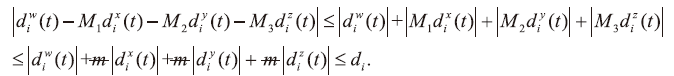
External disturbances ${\rm{\Delta }}{f}_{i}({x}_{i},t),{\rm{\Delta }}{g}_{i}({y}_{i},t),{\rm{\Delta }}{h}_{i}({z}_{i},t),{\rm{\Delta }}{l}_{i}({w}_{i},t)$ are bounded, and there exist positive constants ${d}_{i}^{x},\,{d}_{i}^{y},\,{d}_{i}^{z},{d}_{i}^{w}$ such that $\left|{\rm{\Delta }}{f}_{i}({x}_{i},t)\right|\,\leqslant {d}_{i}^{x},\,\left|{\rm{\Delta }}{g}_{i}({y}_{i},t)\right|\leqslant {d}_{i}^{y},\left|{\rm{\Delta }}{h}_{i}({z}_{i},t)\right|\leqslant {d}_{i}^{z},\left|{\rm{\Delta }}{l}_{i}({w}_{i},t)\right|\leqslant {d}_{i}^{w}.$

Because ${M}_{1},{M}_{2},\text{}{M}_{3}$ are constant matrices, there exists a positive constant , satisfies λmax (${M}_{1},{M}_{2},\text{}{M}_{3}$) . Under Assumption 1, there exists a positive constant , such that

The time-varying delay $\tau (t)$ is a continuously differentiable function and satisfies $0\leqslant \dot{\tau }(t)\leqslant \varepsilon \lt 1,$ so it is easy to get

$\begin{eqnarray}\displaystyle \frac{1-\dot{\tau }(t)}{2(1-\varepsilon )}\geqslant \displaystyle \frac{1}{2},\end{eqnarray}$
where 0 < ϵ < 1 is positive constant. This assumption is still satisfied if τ(t) is zero or some other constants.

Let x(t) ∈ Rn be a differentiable vector. Then, for any time instant tt0 [40]

$\begin{eqnarray}\displaystyle \frac{1}{2}{D}^{\alpha }({x}^{{\rm{T}}}(t)x(t))\leqslant {x}^{{\rm{T}}}(t){D}^{\alpha }x(t),\,\forall \alpha \in (0,1).\end{eqnarray}$
Proof. Proving that expression (8) is true, is equivalent to proving that
$\begin{eqnarray}{x}^{{\rm{T}}}(t){D}^{\alpha }x(t)-\displaystyle \frac{1}{2}{D}^{\alpha }({x}^{{\rm{T}}}(t)x(t))\geqslant 0,\,\forall \alpha \in (0,\,1).\end{eqnarray}$
And in the same way
$\begin{eqnarray*}\begin{array}{l}\displaystyle \frac{1}{2}{D}^{\alpha }({x}^{{\rm{T}}}(t)x(t))=\displaystyle \frac{1}{2}\cdot \displaystyle \frac{1}{{\rm{\Gamma }}(1-\alpha )}\\ \,\times \displaystyle {\int }_{0}^{t}\displaystyle \frac{{\dot{x}}^{{\rm{T}}}(\tau )x(\tau )+{x}^{{\rm{T}}}(\tau )\dot{x}(\tau )}{{(t-\tau )}^{\alpha }}{\rm{d}}\tau ,\end{array}\end{eqnarray*}$
$\begin{eqnarray*}{\dot{x}}^{{\rm{T}}}(\tau )x(\tau )+{x}^{{\rm{T}}}(\tau )\dot{x}(\tau )=2{x}^{{\rm{T}}}(\tau )\dot{x}(\tau ),\end{eqnarray*}$
so
$\begin{eqnarray*}\displaystyle \frac{1}{2}{D}^{\alpha }({x}^{{\rm{T}}}(t)x(t))=\displaystyle \frac{1}{{\rm{\Gamma }}(1-\alpha )}\displaystyle {\int }_{0}^{t}\displaystyle \frac{{x}^{{\rm{T}}}(\tau )\dot{x}(\tau )}{{(t-\tau )}^{\alpha }}{\rm{d}}\tau .\end{eqnarray*}$
So, expression (9) can be written as
$\begin{eqnarray}\displaystyle \frac{1}{{\rm{\Gamma }}(1-\alpha )}\displaystyle {\int }_{0}^{t}\displaystyle \frac{({x}^{{\rm{T}}}(t)-{x}^{{\rm{T}}}(\tau ))\dot{x}(\tau )}{{(t-\tau )}^{\alpha }}{\rm{d}}\tau \geqslant 0.\end{eqnarray}$
Let us define the auxiliary variable $z(\tau )={x}^{{\rm{T}}}(t)\,-{x}^{{\rm{T}}}(\tau ).$ In this way, expression (10) can be written as
$\begin{eqnarray}\displaystyle \frac{1}{{\rm{\Gamma }}(1-\alpha )}\displaystyle {\int }_{0}^{t}\displaystyle \frac{{z}^{{\rm{T}}}(\tau )\dot{z}(\tau )}{{(t-\tau )}^{\alpha }}{\rm{d}}\tau \leqslant 0.\end{eqnarray}$
Let us integrate by parts expression (11), defining
$\begin{eqnarray*}\begin{array}{l}u=\displaystyle \frac{1}{2}{z}^{2},\,{\rm{d}}u={z}^{T}(\tau )\dot{z}(\tau ){\rm{d}}\tau ,\,v=\displaystyle \frac{1}{{\rm{\Gamma }}(1-\alpha )}{(t-\tau )}^{-\alpha },\,\\ {\rm{d}}v=\displaystyle \frac{\alpha }{{\rm{\Gamma }}(1-\alpha )}{(t-\tau )}^{-\alpha -1}.\end{array}\end{eqnarray*}$
In this way, expression (11) can be written as
$\begin{eqnarray}\begin{array}{l}-\left[\displaystyle \frac{-{z}^{2}(\tau )}{2{\rm{\Gamma }}(1-\alpha ){(t-\tau )}^{\alpha }}\right]\left|{\Space{0ex}{1.45em}{0ex}| }_{\tau =t}\right.+\left[\displaystyle \frac{{z}_{0}^{2}}{2{\rm{\Gamma }}(1-\alpha ){t}^{\alpha }}\right]\\ \,+\displaystyle \frac{\alpha }{2{\rm{\Gamma }}(1-\alpha )}\displaystyle {\int }_{0}^{t}\displaystyle \frac{{z}^{2}(\tau )}{{(t-\tau )}^{\alpha }}{\rm{d}}\tau \geqslant 0.\end{array}\end{eqnarray}$
Let us check the first term of expression (10), which has an indetermination at $\tau =t,$ so let us analyze the corresponding limit
$\begin{eqnarray*}\begin{array}{l}\mathop{\mathrm{lim}}\limits_{\tau \to t}\displaystyle \frac{{z}^{2}(\tau )}{2{\rm{\Gamma }}(1-\alpha ){(t-\tau )}^{\alpha }}=\displaystyle \frac{1}{2{\rm{\Gamma }}(1-\alpha )}\\ \times \,\mathop{\mathrm{lim}}\limits_{\tau \to t}\displaystyle \frac{({x}^{2}(t)-2x(t)x(\tau )+{x}^{2}(\tau ))}{{(t-\tau )}^{\alpha }}.\end{array}\end{eqnarray*}$
Given that the function is derivable, L’Hôpital’s rule can be applied. Then
$\begin{eqnarray*}\begin{array}{l}\displaystyle \frac{1}{2{\rm{\Gamma }}(1-\alpha )}\mathop{\mathrm{lim}}\limits_{\tau \to t}\displaystyle \frac{({x}^{2}(t)-2x(t)x(\tau )+{x}^{2}(\tau ))}{{(t-\tau )}^{\alpha }}\\ \,=\,\displaystyle \frac{1}{2{\rm{\Gamma }}(1-\alpha )}\mathop{\mathrm{lim}}\limits_{\tau \to t}\displaystyle \frac{(-2x(t)\dot{x}(\tau )+2x(t)\dot{x}(\tau )){(t-\tau )}^{1-\alpha }}{\alpha }\\ \,=\,0.\end{array}\end{eqnarray*}$
So, expression (12) is reduced to
$\begin{eqnarray}\displaystyle \frac{{z}_{0}^{2}}{2{\rm{\Gamma }}(1-\alpha ){t}^{\alpha }}+\displaystyle \frac{\alpha }{2{\rm{\Gamma }}(1-\alpha )}\displaystyle {\int }_{0}^{t}\displaystyle \frac{{z}^{2}(\tau )}{{(t-\tau )}^{\alpha }}{\rm{d}}\tau \geqslant 0.\end{eqnarray}$
Expression (13) is clearly true, and this concludes the proof.

One can expect an equality in (8) when function $x(t)$ is a constant or when $\alpha =1.$

The case when $\alpha =1$ corresponds to the product rule for the integer order derivatives, which states that $\displaystyle \frac{1}{2}\displaystyle \frac{{\rm{d}}{x}^{T}(t)x(t)}{{\rm{d}}t}\,={x}^{T}(t)\displaystyle \frac{{\rm{d}}x(t)}{{\rm{d}}t},$ so it can be considered as a particular case of Lemma 1.

3. Controller design

To realize combined projective synchronization, the controller and parameter adaptive laws are designed as follows:
$\begin{eqnarray}\begin{array}{l}{u}_{i}(t)=-{l}_{i}({w}_{i})-{\hat{d}}_{i}sign({e}_{i}(t))-{\hat{q}}_{i}{e}_{i}(t)+{M}_{1}f({x}_{i})\\ \,+\,{M}_{2}g({y}_{i})+{M}_{3}h({z}_{i}),\end{array}\end{eqnarray}$
$\begin{eqnarray}{D}^{\alpha }{\hat{d}}_{i}={k}_{1}{{e}_{i}}^{{\rm{T}}}(t)sign({e}_{i}(t)),\end{eqnarray}$
$\begin{eqnarray}{D}^{\alpha }{\hat{q}}_{i}={k}_{2}{{e}_{i}}^{{\rm{T}}}(t){e}_{i}(t).\end{eqnarray}$
Theorem 1. If assumptions 1–2 are satisfied, the drive system (1)–(3) and the response system (4) can realize function projective synchronization with the controller (14) and adaptive laws (15)–(16).
Proof. From Definition 1, we have the error term:
$\begin{eqnarray}{e}_{i}(t)={w}_{i}(t)-({M}_{1}{x}_{i}(t)+{M}_{2}{y}_{i}(t)+{M}_{3}{z}_{i}(t)).\end{eqnarray}$
The α-order derivatives of ${e}_{i}(t)$ is:
$\begin{eqnarray*}\begin{array}{l}{D}^{\alpha }{e}_{i}(t)={D}^{\alpha }{w}_{i}(t)-\left({D}^{\alpha }\right.{M}_{1}{x}_{i}(t)+{D}^{\alpha }{M}_{2}{y}_{i}(t)\\ \,+\,{D}^{\alpha }{M}_{3}{z}_{i}\left.(t\right)\\ \,=\,{l}_{i}({w}_{i})+{\rm{\Delta }}{l}_{i}({w}_{i},t)+{c}_{1}\displaystyle \sum _{j=1}^{N}{a}_{ij}{{\rm{\Gamma }}}_{1}{w}_{j}(t)\\ \,+\,{c}_{2}\displaystyle \sum _{j=1}^{N}{b}_{ij}{{\rm{\Gamma }}}_{2}{w}_{j}(t-\tau (t))+{u}_{i}(t)\\ \,-\,({D}^{\alpha }{M}_{1}{x}_{i}(t)+{D}^{\alpha }{M}_{2}{y}_{i}(t)+{D}^{\alpha }{M}_{3}{z}_{i}(t))\\ \,=\,{l}_{i}({w}_{i})+{\rm{\Delta }}{l}_{i}({w}_{i},t)+{c}_{1}\displaystyle \sum _{j=1}^{N}{a}_{ij}{{\rm{\Gamma }}}_{1}{w}_{j}(t)\\ \,+\,{c}_{2}\displaystyle \sum _{j=1}^{N}{b}_{ij}{{\rm{\Gamma }}}_{2}{w}_{j}(t-\tau (t))-{l}_{i}({w}_{i})-{\hat{d}}_{i}\mathrm{sign}({e}_{i}(t))\\ \,-\,{\hat{q}}_{i}{e}_{i}(t)\\ \,+\,{M}_{1}{f}_{1}({x}_{i})+{M}_{2}{g}_{1}({y}_{i})+{M}_{3}{h}_{1}({z}_{i})-\left({D}^{\alpha }\right.{M}_{1}{x}_{i}(t)\\ \,+\,{D}^{\alpha }{M}_{2}{y}_{i}(t)+\left.{D}^{\alpha }{M}_{3}{z}_{i}(t)\right)\\ =\,{\rm{\Delta }}{l}_{i}({w}_{i},t)-\left({M}_{1}\right.{\rm{\Delta }}{f}_{i}({x}_{i},t)+{M}_{2}{\rm{\Delta }}{g}_{i}({y}_{i},t)\\ \,+\,{M}_{3}{\rm{\Delta }}{h}_{i}\left.({z}_{i},t\right)-{\hat{d}}_{i}\mathrm{sign}({e}_{i}(t))-{\hat{q}}_{i}{e}_{i}(t)\\ \,+\,{c}_{1}\displaystyle \sum _{j=1}^{N}{a}_{ij}{{\rm{\Gamma }}}_{1}{w}_{j}(t)-\left({c}_{1}\right.\displaystyle \sum _{j=1}^{N}{a}_{ij}{{\rm{\Gamma }}}_{1}{M}_{1}{x}_{j}(t)\\ \,+\,{c}_{1}\displaystyle \sum _{j=1}^{N}{a}_{ij}{{\rm{\Gamma }}}_{1}{M}_{2}{y}_{j}(t)+{c}_{1}\displaystyle \sum _{j=1}^{N}{a}_{ij}{{\rm{\Gamma }}}_{1}{M}_{3}{z}_{j}\left.(t\right)\\ +\,{c}_{2}\displaystyle \sum _{j=1}^{N}{b}_{ij}{{\rm{\Gamma }}}_{2}{w}_{j}(t-\tau (t))-\left({c}_{2}\right.\displaystyle \sum _{j=1}^{N}{b}_{ij}{{\rm{\Gamma }}}_{2}{M}_{1}{x}_{j}(t-\tau (t))\\ \,+\,{c}_{2}\displaystyle \sum _{j=1}^{N}{b}_{ij}{{\rm{\Gamma }}}_{2}{M}_{2}{y}_{j}(t-\tau (t))+{c}_{2}\displaystyle \sum _{j=1}^{N}{b}_{ij}{{\rm{\Gamma }}}_{2}{M}_{3}{z}_{j}\left.(t-\tau (t)\right).\end{array}\end{eqnarray*}$
Choosing Lyapunov function as:
$\begin{eqnarray*}\begin{array}{l}V=\displaystyle \frac{1}{2}\displaystyle \sum _{i=1}^{N}{{e}_{i}}^{{\rm{T}}}(t){e}_{i}(t)+\displaystyle \frac{1}{2{k}_{1}}\displaystyle \sum _{i=1}^{N}{\tilde{d}}_{i}^{2}+\displaystyle \frac{1}{2{k}_{2}}\displaystyle \sum _{i=1}^{N}\left({\hat{q}}_{i}\right.-{\left.{q}^{\ast }\right)}^{2}\\ \,+{}_{{t}_{0}}{}^{R}I_{t}^{\alpha -1}\displaystyle \frac{1}{2(1-\varepsilon )}\displaystyle {\int }_{t-\tau }^{t}\displaystyle \sum _{i=1}^{N}{{e}_{i}}^{{\rm{T}}}(\delta ){e}_{i}(\delta ){\rm{d}}\delta .\end{array}\end{eqnarray*}$
Taking the derivative of the Lyapunov function, we can get:
$\begin{eqnarray*}\begin{array}{l}{D}^{\alpha }V=\displaystyle \sum _{i=1}^{N}{{e}_{i}}^{{\rm{T}}}(t){D}^{\alpha }{e}_{i}(t)+\displaystyle \frac{1}{{k}_{1}}\displaystyle \sum _{i=1}^{N}({\hat{d}}_{i}-{d}_{i}){D}^{\alpha }{\hat{d}}_{i}\\ \,+\,\displaystyle \frac{1}{{k}_{2}}\displaystyle \sum _{i=1}^{N}({\hat{q}}_{i}-{q}^{\ast }){D}^{\alpha }{\hat{q}}_{i}\\ \,+\,\displaystyle \frac{{\rm{d}}\displaystyle \frac{1}{2(1-\varepsilon )}\displaystyle {\int }_{t-\tau }^{t}\displaystyle \sum _{i=1}^{N}{{e}_{i}}^{T}(\delta ){e}_{i}(\delta ){\rm{d}}\delta }{{\rm{d}}t}\\ =\,\displaystyle \sum _{i=1}^{N}{{e}_{i}}^{{\rm{T}}}(t)\left({\rm{\Delta }}{l}_{i}\right.({w}_{i},t)-\left({M}_{1}{\rm{\Delta }}{f}_{i}\right.({x}_{i},t)+{M}_{2}{\rm{\Delta }}{g}_{i}({y}_{i},t)\\ \,+\,{M}_{3}{\rm{\Delta }}{h}_{i}\left.({z}_{i},t\right)-{\hat{d}}_{i}\mathrm{sign}({e}_{i}(t))-{\hat{q}}_{i}{e}_{i}(t)\\ +\,{c}_{1}\displaystyle \sum _{j=1}^{N}{a}_{ij}{{\rm{\Gamma }}}_{1}{w}_{j}(t)-\left({c}_{1}\right.\displaystyle \sum _{j=1}^{N}{a}_{ij}{{\rm{\Gamma }}}_{1}{M}_{1}{x}_{j}(t)\\ \,+\,{c}_{1}\displaystyle \sum _{j=1}^{N}{a}_{ij}{{\rm{\Gamma }}}_{1}{M}_{2}{y}_{j}(t)+{c}_{1}\displaystyle \sum _{j=1}^{N}{a}_{ij}{{\rm{\Gamma }}}_{1}{M}_{3}{z}_{j}\left.(t\right)\\ +\,{c}_{2}\displaystyle \sum _{j=1}^{N}{b}_{ij}{{\rm{\Gamma }}}_{2}{w}_{j}(t-\tau (t))-\left({c}_{2}\right.\displaystyle \sum _{j=1}^{N}{b}_{ij}{{\rm{\Gamma }}}_{2}{M}_{1}{x}_{j}(t-\tau (t))\\ \,+\,{c}_{2}\displaystyle \sum _{j=1}^{N}{b}_{ij}{{\rm{\Gamma }}}_{2}{M}_{2}{y}_{j}(t-\tau (t))\\ \,+\,{c}_{2}\displaystyle \sum _{j=1}^{N}{b}_{ij}{{\rm{\Gamma }}}_{2}{M}_{3}{z}_{j}\left.\left.(t-\tau (t)\right)\right)\\ \,+\,\displaystyle \frac{1}{{k}_{1}}\displaystyle \sum _{i=1}^{N}({\hat{d}}_{i}-{d}_{i}){k}_{1}{{e}_{i}}^{{\rm{T}}}(t)\mathrm{sign}({e}_{i}(t))\\ \,+\,\displaystyle \frac{1}{{k}_{2}}\displaystyle \sum _{i=1}^{N}({\hat{q}}_{i}-{q}^{\ast })\cdot {k}_{2}{{e}_{i}}^{{\rm{T}}}(t){e}_{i}(t)\\ \,+\,\displaystyle \frac{1}{2(1-\varepsilon )}\displaystyle \sum _{i=1}^{N}{{e}_{i}}^{{\rm{T}}}(t){e}_{i}(t)-\displaystyle \frac{1-\dot{\tau }(t)}{2(1-\varepsilon )}\\ \,\times \,\displaystyle \sum _{i=1}^{N}{{e}_{i}}^{{\rm{T}}}(t-\tau (t)){e}_{i}(t-\tau (t)).\end{array}\end{eqnarray*}$
Because
Then
$\begin{eqnarray*}\begin{array}{l}{D}^{\alpha }V=\displaystyle \sum _{i=1}^{N}{{e}_{i}}^{{\rm{T}}}(t)\left({d}_{i}\right.-{\hat{d}}_{i}\mathrm{sign}({e}_{i}(t))-{\hat{q}}_{i}{e}_{i}(t)\\ \,+{c}_{1}\displaystyle \sum _{j=1}^{N}{a}_{ij}{{\rm{\Gamma }}}_{1}{e}_{j}(t)+{c}_{2}\displaystyle \sum _{j=1}^{N}{b}_{ij}{{\rm{\Gamma }}}_{2}{e}_{j}\left.(t-\tau (t)\right)\\ +\displaystyle \frac{1}{{k}_{1}}\displaystyle \sum _{i=1}^{N}({\hat{d}}_{i}-{d}_{i}){k}_{1}{{e}_{i}}^{{\rm{T}}}(t)\mathrm{sign}({e}_{i}(t))\\ \,+\displaystyle \frac{1}{{k}_{2}}\displaystyle \sum _{i=1}^{N}({\hat{q}}_{i}-{q}^{\ast }){k}_{2}{{e}_{i}}^{{\rm{T}}}(t){e}_{i}(t)\\ +\displaystyle \frac{1}{2(1-\varepsilon )}\displaystyle \sum _{i=1}^{N}{{e}_{i}}^{{\rm{T}}}(t){e}_{i}(t)-\displaystyle \frac{1-\dot{\tau }(t)}{2(1-\varepsilon )}\displaystyle \sum _{i=1}^{N}{{e}_{i}}^{{\rm{T}}}(t-\tau (t)){e}_{i}(t-\tau (t))\\ =\displaystyle \sum _{i=1}^{N}{d}_{i}{{e}_{i}}^{{\rm{T}}}(t)+\displaystyle \sum _{i=1}^{N}{c}_{1}{{e}_{i}}^{{\rm{T}}}(t)\displaystyle \sum _{j=1}^{N}{a}_{ij}{{\rm{\Gamma }}}_{1}{e}_{j}(t)+\displaystyle \sum _{i=1}^{N}(-{d}_{i})\cdot {{e}_{i}}^{{\rm{T}}}(t)\mathrm{sign}({e}_{i}(t))\\ \,+\displaystyle \sum _{i=1}^{N}{c}_{2}{{e}_{i}}^{{\rm{T}}}(t)\displaystyle \sum _{j=1}^{N}{b}_{ij}{{\rm{\Gamma }}}_{2}{e}_{j}(t-\tau (t))\\ +\displaystyle \sum _{i=1}^{N}(-{q}^{\ast }){{e}_{i}}^{{\rm{T}}}(t){e}_{i}(t)+\displaystyle \frac{1}{2(1-\varepsilon )}\displaystyle \sum _{i=1}^{N}{{e}_{i}}^{{\rm{T}}}(t){e}_{i}(t)\\ \,-\displaystyle \frac{1-\dot{\tau }(t)}{2(1-\varepsilon )}\displaystyle \sum _{i=1}^{N}{{e}_{i}}^{{\rm{T}}}(t-\tau (t)){e}_{i}(t-\tau (t)).\end{array}\end{eqnarray*}$
Let $e(t)={({e}_{1}^{{\rm{T}}}(t),\,{e}_{2}^{{\rm{T}}}(t),\,\mathrm{..}.,\,{e}_{N}^{{\rm{T}}}(t))}^{{\rm{T}}}\in {{\bf{R}}}^{N\times 1},$ $P=({A}_{1}\otimes {{\rm{\Gamma }}}_{1}),Q=({B}_{1}\otimes {{\rm{\Gamma }}}_{2}),$ where $\otimes $ represents the Kronecker product, then we can get:
$\begin{eqnarray*}\begin{array}{l}\displaystyle \sum _{i=1}^{N}{c}_{2}{{e}_{i}}^{{\rm{T}}}(t)\displaystyle \sum _{j=1}^{N}{b}_{ij}{{\rm{\Gamma }}}_{2}{e}_{j}(t-\tau (t))={c}_{2}{e}^{{\rm{T}}}(t)Q{e}^{{\rm{T}}}(t-\tau (t))\\ \,\leqslant \displaystyle \frac{1}{2}{c}_{2}^{2}{e}^{{\rm{T}}}(t){Q}^{{\rm{T}}}Qe(t)+\displaystyle \frac{1}{2}{e}^{{\rm{T}}}(t-\tau (t))e(t-\tau (t)).\end{array}\end{eqnarray*}$
Then,
$\begin{array}{l}\displaystyle \sum _{i=1}^{N}{d}_{i}{{e}_{i}}^{{\rm{T}}}(t)\leqslant \displaystyle \sum _{i=1}^{N}{d}_{i}{{e}_{i}}^{{\rm{T}}}(t)\mathrm{sign}({e}_{i}(t)).\\ {D}^{\alpha }V\leqslant \displaystyle \sum _{i=1}^{N}{c}_{1}{{e}_{i}}^{{\rm{T}}}(t)\displaystyle \sum _{j=1}^{N}{a}_{ij}{{\rm{\Gamma }}}_{1}{e}_{j}(t)+\displaystyle \sum _{i=1}^{N}(-{q}^{\ast })\cdot {{e}_{i}}^{{\rm{T}}}(t){{e}_{i}}^{{\rm{T}}}(t)\\ \,+\displaystyle \frac{1}{2(1-\varepsilon )}\displaystyle \sum _{i=1}^{N}{{e}_{i}}^{{\rm{T}}}(t){e}_{i}(t)-\displaystyle \frac{1-\dot{\tau }(t)}{2(1-\varepsilon )}\displaystyle \sum _{i=1}^{N}{{e}_{i}}^{{\rm{T}}}(t-\tau (t)){e}_{i}\\ \,\times \,(t-\tau (t))\\ \,+\displaystyle \frac{1}{2}{c}_{2}^{2}{e}^{{\rm{T}}}(t){Q}^{{\rm{T}}}Qe(t)+\displaystyle \frac{1}{2}{e}^{{\rm{T}}}(t-\tau (t))e(t-\tau (t))\\ \,={c}_{1}{e}^{{\rm{T}}}(t)Pe(t)+(-{q}^{\ast }){e}^{{\rm{T}}}(t)e(t)+\displaystyle \frac{1}{2(1-\varepsilon )}{e}^{{\rm{T}}}(t)e(t)\\ \,-\displaystyle \frac{1-\dot{\tau }(t)}{2(1-\varepsilon )}{e}^{{\rm{T}}}(t-\tau (t))e(t-\tau (t))\\ \,+\displaystyle \frac{1}{2}{c}_{2}^{2}{e}^{{\rm{T}}}(t){Q}^{{\rm{T}}}Qe(t)+\displaystyle \frac{1}{2}{e}^{{\rm{T}}}(t-\tau (t))e(t-\tau (t)).\end{array}$
Because
$\displaystyle \frac{1-\dot{\tau }(t)}{2(1-\varepsilon )}\geqslant \displaystyle \frac{1}{2},$ then $-\displaystyle \frac{1-\dot{\tau }(t)}{2(1-\varepsilon )}\displaystyle {\sum }_{i=1}^{N}{{e}_{i}}^{{\rm{T}}}(t-\tau (t)){e}_{i}(t-\tau (t))+\displaystyle \frac{1}{2}{e}^{{\rm{T}}}(t-\tau (t))e(t-\tau (t))\leqslant 0.$
$\begin{eqnarray*}\begin{array}{l}{D}^{\alpha }V\leqslant {c}_{1}{e}^{{\rm{T}}}(t)Pe(t)-{q}^{\ast }{e}^{{\rm{T}}}(t)e(t)\\ +\displaystyle \frac{1}{2}{c}_{2}^{2}{e}^{{\rm{T}}}(t){Q}^{{\rm{T}}}Qe(t)+\displaystyle \frac{1}{2(1-\varepsilon )}{e}^{{\rm{T}}}(t)e(t),\\ {q}^{\ast }\geqslant {\lambda }_{\max }\left(\displaystyle \frac{1}{2}{c}_{2}^{2}{Q}^{{\rm{T}}}Q+{c}_{1}P\right)+\displaystyle \frac{1}{2(1-\varepsilon )}.\end{array}\end{eqnarray*}$
If ${q}^{\ast }\geqslant {\lambda }_{\max }\left(\displaystyle \frac{1}{2}{c}_{2}^{2}{Q}^{{\rm{T}}}Q+{c}_{1}P\right)+\displaystyle \frac{1}{2(1-\varepsilon )},$ we can get ${D}^{\alpha }V(t)\leqslant 0,$ where ${\lambda }_{\max }\left(\displaystyle \frac{1}{2}{c}_{2}^{2}{Q}^{{\rm{T}}}Q+{c}_{1}P\right)$ is the maximum eigenvalue of Matrix $\displaystyle \frac{1}{2}{c}_{2}^{2}{Q}^{{\rm{T}}}Q+{c}_{1}P.$
Based on the above analysis, we can get that ${D}^{\alpha }V(t)\leqslant 0$ if ${q}^{\ast }\geqslant {\lambda }_{\max }\left(\displaystyle \frac{1}{2}{c}_{2}^{2}{Q}^{{\rm{T}}}Q+{c}_{1}P\right)+\displaystyle \frac{1}{2(1-\varepsilon )}.$ According to Lyapunov stability theory, we can obtain ${e}_{i}(t)\to 0$ as $t\to \infty ,$ which means that the combination projective synchronization between the drive system (1)–(3) and the response system (4) is achieved. This completes the proof.

With the differences of ${M}_{1},{M}_{2},{M}_{3},$ combination projection synchronization can be changed into (a) combination complete synchronization (${M}_{1}={M}_{2}={M}_{3}=I,$ $I$ is an identity matrix), (b) combination anti-synchronization(${M}_{1}={M}_{2}={M}_{3}=-I$), (c) projective synchronization (there are two zero matrices in ${M}_{1},{M}_{2},{M}_{3}.$), and (d) control problem(${M}_{1},{M}_{2},{M}_{3}$ are all zero matrices.).

At present, there is little research on combination synchronization for fractional-order complex networks. Combination synchronization can realize synchronization between multi-drive and multi-response systems, which is a more generalized form of synchronization.

When $\tau (t)$ is constant, the time-varying delay couplings problem is transformed into constant time-delay coupling. When $\tau (t)$ is constant, Assumption 2 is also satisfied, the control method in this article is also applicable to constant time-delay coupling.

The combination projective synchronization can be extended to synchronize among many different complex networks, that is $e=\displaystyle {\sum }_{i=1}^{n}{x}_{i}-\displaystyle {\sum }_{j=1}^{m}{y}_{j}=0,$ where ${x}_{i},$ ${y}_{j}$ represent drive systems and response systems respectively and $m,n$ are positive integers [31].

4. Numerical simulation

In this section, two fractional-order complex network combination projection synchronization examples will be provided to demonstrate the effectiveness of the provided theorem and corollary.

Considering a fractional-order complex dynamic network with $N=3,n=3,$ the three drive systems are composed of three chaotic systems with time-varying delay couplings.

$\begin{eqnarray*}\begin{array}{l}\left[\begin{array}{l}{D}^{\alpha }{x}_{i1}\,(t)\\ {D}^{\alpha }{x}_{i2}\,(t)\\ {D}^{\alpha }{x}_{i3}\,(t)\end{array}\right]\,=\,\left[\begin{array}{c}10(-{x}_{i1}\,(t)+{x}_{i2}\,(t))\\ 28{x}_{i1}\,(t)-{x}_{i1}\,(t){x}_{i3}\,(t)-{x}_{i2}\,(t)\\ {x}_{i1}\,(t){x}_{i2}\,(t)-\displaystyle \frac{8}{3}{x}_{i3}\,(t)\end{array}\right]\\ \,+\,\left[\begin{array}{l}{d}_{i1}^{x}(t)\\ {d}_{i2}^{x}(t)\\ {d}_{i3}^{x}(t)\end{array}\right]\\ \,+\,{c}_{1}(t)\displaystyle \sum _{j=1}^{3}{a}_{ij}^{1}{{\rm{\Gamma }}}_{1}{x}_{j}(t)+{c}_{2}(t)\displaystyle \sum _{j=1}^{3}{b}_{ij}^{1}{{\rm{\Gamma }}}_{2}{x}_{j}(t-\tau (t)).\\ i=1,2,3.\end{array}\end{eqnarray*}$
$\begin{eqnarray*}\begin{array}{l}\left[\begin{array}{l}{D}^{\alpha }{y}_{i1}(t)\\ {D}^{\alpha }{y}_{i2}(t)\\ {D}^{\alpha }{y}_{i3}(t)\end{array}\right]=\left[\begin{array}{c}35({y}_{i2}(t)-{y}_{i1}(t))\\ -10{y}_{i1}(t)+25{y}_{i2}(t)-{y}_{i1}(t){y}_{i3}(t)\\ {y}_{i1}(t){y}_{i2}(t)-3{y}_{i2}(t)\end{array}\right]\\ \,+\,\left[\begin{array}{l}{d}_{i1}^{y}(t)\\ {d}_{i2}^{y}(t)\\ {d}_{i3}^{y}(t)\end{array}\right]\\ \,+\,{c}_{1}(t)\displaystyle \sum _{j=1}^{3}{a}_{ij}^{1}{{\rm{\Gamma }}}_{1}{y}_{j}(t)+{c}_{2}(t)\displaystyle \sum _{j=1}^{3}{b}_{ij}^{1}{{\rm{\Gamma }}}_{2}{y}_{j}(t-\tau (t)).\\ i=1,2,3.\end{array}\end{eqnarray*}$
$\begin{eqnarray*}\begin{array}{l}\left[\begin{array}{l}{D}^{\alpha }{z}_{i1}(t)\\ {D}^{\alpha }{z}_{i2}(t)\\ {D}^{\alpha }{z}_{i3}(t)\end{array}\right]\,=\,\left[\begin{array}{c}36({z}_{i2}(t)-{z}_{i1}(t))\\ 20{z}_{i2}(t)-{z}_{i1}(t){z}_{i3}(t)\\ {z}_{i1}(t){z}_{i2}(t)-3{z}_{i2}(t)\end{array}\right]+\left[\begin{array}{l}{d}_{i1}^{z}(t)\\ {d}_{i2}^{z}(t)\\ {d}_{i3}^{z}(t)\end{array}\right]\\ \,+\,{c}_{1}(t)\displaystyle \sum _{j=1}^{3}{a}_{ij}^{1}{{\rm{\Gamma }}}_{1}{z}_{j}(t)+{c}_{2}(t)\displaystyle \sum _{j=1}^{3}{b}_{ij}^{1}{{\rm{\Gamma }}}_{2}{z}_{j}(t-\tau (t)).\\ i=1,2,3.\end{array}\end{eqnarray*}$
The response system is composed of chaotic systems with time-varying delay couplings.
$\begin{eqnarray*}\begin{array}{l}\left[\begin{array}{l}{D}^{\alpha }{w}_{i1}(t)\\ {D}^{\alpha }{w}_{i2}(t)\\ {D}^{\alpha }{w}_{i3}(t)\end{array}\right]\,=\,\left[\begin{array}{c}-{w}_{i2}(t)-{w}_{i3}(t)\\ {w}_{i1}(t)+0.2{w}_{i2}(t)\\ {w}_{i1}(t){w}_{i3}(t)-5.7{y}_{i3}(t)+0.2\end{array}\right]\\ \,+\,\left[\begin{array}{l}{d}_{i1}^{w}(t)\\ {d}_{i2}^{w}(t)\\ {d}_{i3}^{w}(t)\end{array}\right]\\ \,+\,{c}_{1}(t)\displaystyle \sum _{j=1}^{3}{a}_{ij}^{1}{{\rm{\Gamma }}}_{1}{w}_{j}(t)+{c}_{2}(t)\displaystyle \sum _{j=1}^{3}{b}_{ij}^{1}{{\rm{\Gamma }}}_{2}{w}_{j}(t-\tau (t)).\\ i=1,2,3.\end{array}\end{eqnarray*}$
In the numerical simulation, set ${c}_{1}={c}_{2}=0.2,$ $\tau (t)=\displaystyle \frac{t}{3+t},$ ${d}_{i}(t)=0.2\,\cos \,t,$ ${{\rm{\Gamma }}}_{1}={{\rm{\Gamma }}}_{2}={I}^{3\times 3}.$ The topological structure matrices ${A}_{1},$ ${A}_{2}$ are as follows and the topological relationship of nodes are shown in figure 1:
$\begin{eqnarray*}{A}_{1}=\left(\begin{array}{ccc}-1 & 0 & 1\\ 0 & -1 & 1\\ 1 & 1 & -2\end{array}\right),\,{A}_{2}=\left(\begin{array}{ccc}-2 & 1 & 1\\ 1 & -1 & 0\\ 0 & 1 & -1\end{array}\right).\end{eqnarray*}$
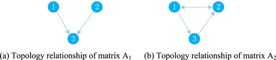
Figure 1. Topological relationship between nodes.
The simulation results are shown in figure 2. It displays that the error signal between the drive systems and the response system can stably approach zero with the designed adaptive controller, that is, the combination projection synchronization of the complex dynamic networks is realized.

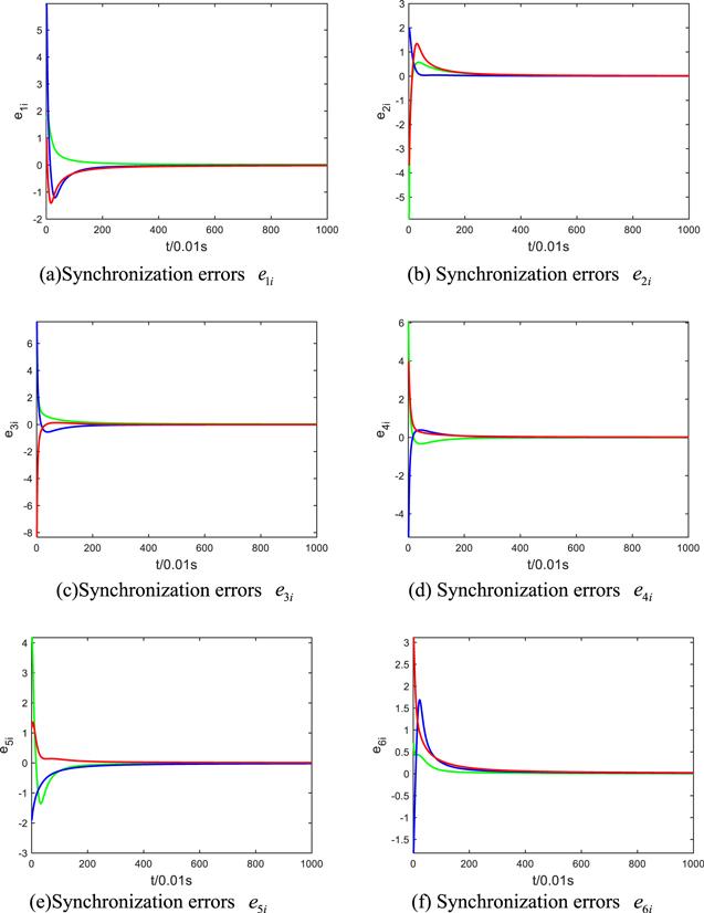
Considering a fractional-order complex dynamic network with $N=6,n=3,$ the drive systems are composed of six chaotic systems with time-varying delay couplings.

$\begin{eqnarray*}\begin{array}{l}\left[\begin{array}{l}{D}^{\alpha }{x}_{i1}(t)\\ {D}^{\alpha }{x}_{i2}(t)\\ {D}^{\alpha }{x}_{i3}(t)\end{array}\right]\,=\,\left[\begin{array}{c}0\\ -{x}_{i1}(t){x}_{i3}(t)\\ {x}_{i1}(t){x}_{i2}(t)\end{array}\right]+\left[\begin{array}{l}{d}_{i1}^{x}(t)\\ {d}_{i2}^{x}(t)\\ {d}_{i3}^{x}(t)\end{array}\right]\\ \,+{c}_{1}(t)\displaystyle \sum _{j=1}^{6}{a}_{ij}^{1}{{\rm{\Gamma }}}_{1}{x}_{j}(t)+{c}_{2}(t)\displaystyle \sum _{j=1}^{6}{a}_{ij}^{2}{{\rm{\Gamma }}}_{2}{x}_{j}(t-\tau (t)).\\ i=1,2,\cdots ,6.\end{array}\end{eqnarray*}$
$\begin{eqnarray*}\begin{array}{l}\left[\begin{array}{l}{D}^{\alpha }{y}_{i1}(t)\\ {D}^{\alpha }{y}_{i2}(t)\\ {D}^{\alpha }{y}_{i3}(t)\end{array}\right]\,=\,\left[\begin{array}{c}0\\ {y}_{i2}(t)-{y}_{i1}(t){y}_{i3}(t)-{y}_{i4}(t)\\ {y}_{i1}(t){y}_{i2}(t)\end{array}\right]+\left[\begin{array}{l}{d}_{i1}^{y}(t)\\ {d}_{i2}^{y}(t)\\ {d}_{i3}^{y}(t)\end{array}\right]\\ \,+{c}_{1}(t)\displaystyle \sum _{j=1}^{6}{a}_{ij}^{1}{{\rm{\Gamma }}}_{1}{y}_{j}(t)+{c}_{2}\left(t\right)\displaystyle \sum _{j=1}^{6}{a}_{ij}^{2}{{\rm{\Gamma }}}_{2}{y}_{j}(t-\tau (t)).\\ i=1,2,\cdots ,6.\end{array}\end{eqnarray*}$
$\begin{eqnarray*}\begin{array}{l}\left[\begin{array}{l}{D}^{\alpha }{z}_{i1}(t)\\ {D}^{\alpha }{z}_{i2}(t)\\ {D}^{\alpha }{z}_{i3}(t)\end{array}\right]\,=\,\left[\begin{array}{c}0\\ {z}_{i2}(t)-{z}_{i1}(t){z}_{i3}(t)\\ {z}_{i1}(t){z}_{i2}(t)\end{array}\right]+\left[\begin{array}{l}{d}_{i1}^{z}(t)\\ {d}_{i2}^{z}(t)\\ {d}_{i3}^{z}(t)\end{array}\right]\\ \,+{c}_{1}(t)\displaystyle \sum _{j=1}^{6}{a}_{ij}^{1}{{\rm{\Gamma }}}_{1}{z}_{j}(t)+{c}_{2}(t)\displaystyle \sum _{j=1}^{6}{a}_{ij}^{2}{{\rm{\Gamma }}}_{2}{z}_{j}(t-\tau (t)).\\ i=1,2,\cdots ,6.\end{array}\end{eqnarray*}$
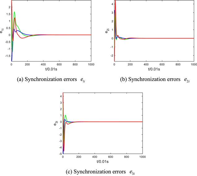
Figure 2. When q = 0.88, the trajectory of each node for the error system.
The response system is composed of six chaotic systems with time-varying delay couplings.
$\begin{eqnarray*}\begin{array}{l}\left[\begin{array}{l}{D}^{\alpha }{w}_{i1}(t)\\ {D}^{\alpha }{w}_{i2}(t)\\ {D}^{\alpha }{w}_{i3}(t)\end{array}\right]\,=\,\left[\begin{array}{c}36({w}_{i2}(t)-{w}_{i1}(t))\\ 20{w}_{i2}(t)-{w}_{i1}(t){w}_{i3}(t)\\ {w}_{i1}(t){w}_{i2}(t)-3{w}_{i3}(t)\end{array}\right]+\left[\begin{array}{l}{d}_{i1}^{w}(t)\\ {d}_{i2}^{w}(t)\\ {d}_{i3}^{w}(t)\end{array}\right]\\ \,+{c}_{1}(t)\displaystyle \sum _{j=1}^{6}{a}_{ij}^{1}{{\rm{\Gamma }}}_{1}{w}_{j}(t)+{c}_{2}t-\tau (t)\displaystyle \sum _{j=1}^{6}{a}_{ij}^{2}{{\rm{\Gamma }}}_{2}{w}_{j}(t-\tau (t)).\\ i=1,2,\cdots ,6.\end{array}\end{eqnarray*}$
To simplify numerical simulation, set ${c}_{1}\,=\,{c}_{2}\,=0.1,{\tau }_{1}(t)=\displaystyle \frac{t}{3+t},{d}_{i}^{x}(t)=0.2\,\sin \,t,{d}_{i}^{y}(t)=0.1\,\sin \,t,$ ${d}_{i}^{z}(t)=0.3\,\cos \,t,{d}_{i}^{w}(t)=0.2\,\cos \,t,{{\rm{\Gamma }}}_{1}={{\rm{\Gamma }}}_{2}={I}^{6\times 6}.$ The topological structure matrices ${A}_{1},{A}_{2}$ are as follows and the topological relationship between nodes is shown in figure 3:
$\begin{eqnarray*}\begin{array}{l}{A}_{1}=\left(\begin{array}{cccccc}-1 & 0 & 0 & 0 & 0 & 1\\ 1 & -1 & 0 & 0 & 0 & 0\\ 0 & 0 & -1 & 1 & 0 & 0\\ 0 & 1 & 0 & -1 & 0 & 0\\ 1 & 0 & 1 & 0 & -2 & 0\\ 0 & 1 & 0 & 1 & 0 & -2\end{array}\right),\\ {A}_{2}=\left(\begin{array}{cccccc}-1 & 0 & 0 & 0 & 1 & 0\\ 0 & -1 & 1 & 0 & 0 & 0\\ 0 & 0 & -1 & 1 & 0 & 0\\ 0 & 1 & 0 & -1 & 0 & 0\\ 0 & 0 & 0 & 0 & -1 & 1\\ 0 & 0 & 1 & 1 & 0 & -2\end{array}\right).\end{array}\end{eqnarray*}$
Figure 3. Topological relationship between nodes.
The simulation results are shown in figure 4. It can still achieve combination projection synchronization when increasing the number of nodes and system dimensions of the complex networks, which further verifies the correctness of the theoretical analysis.
Figure 4. When q = 0.95, the trajectory of each node for the error system.

5. Conclusion

In this paper, the combination projection synchronization of fractional-order complex dynamic networks with time-varying delay couplings and disturbances is investigated. By using Lyapunov stability theory and fractional integral theory, the adaptive controller is designed to realize the combination projection synchronization among four fractional-order complex dynamic networks. The simulation examples show that the drive systems and response systems can be synchronized according to the scaling factors under the controller. The controller does not have a time-delay term, so it is easier to realize in engineering applications. This paper expands the number of synchronization systems and studies the combination projection synchronization between multiple fractional-order complex networks, which increases the complexity of the synchronization systems and provides a new idea for the application of fractional-order complex network synchronization in intelligent optimization, biomedical science and information science fields. In future studies, we will focus on addressing the following two problems: (1) How to realize the synchronization of fractional-order discrete systems? (2) How to solve the synchronization problem under input constraint?

Conflicts of interest

The authors declare there is no conflict of interest regarding the publication of this paper.

The work was supported in part by the National Natural Science Foundation of China (Grant no. 61775198, 62076222, 61903342), Henan Province Science and technology research project (Grant no. 222102210059, 222102210266, 212102310455)

1
Kim P Kim S 2015 Detecting overlapping and hierarchical communities in complex network using interaction-based edge clustering Physica A 417 46 56

DOI

2
Lozano S 2009 Dynamics of social complex networks: some insights into recent research MSSET 42 133 143

DOI

3
Luo Y-Q Wang Z-D Chen Y Yi X-J 2021 H∞ state estimation for coupled stochastic complex networks with periodical communication protocol and intermittent nonlinearity switching IEEE Trans. Netw. Sci. Eng. 8 1414 1425

DOI

4
Ravandi B Ansari F S Mili F 2019 Controllability analysis of complex networks using statistical random sampling Adv. Complex Syst. 22 1950012

DOI

5
Wang G Lu S-W Liu W-B Ma R-N 2021 Adaptive complete synchronization of two complex networks with uncertain parameters, structures, and disturbances J. Comput. Sci. 54 101436

DOI

6
Lu W-L Chen T-P 2021 QUAD-condition, synchronization, consensus of multiagents, and anti-synchronization of complex networks IEEE Trans. Cybernetics 51 3384 3388

DOI

7
Shi H-J Miao L-Y Sun Y-Z Liu M-X 2018 Fixed-time outer synchronization of complex networks with noise coupling Commun. Theor. Phys. 69 271 279

DOI

8
Cheng Q-X Cao J-D 2011 Global synchronization of complex networks with discrete time delays and stochastic disturbances Neural Comput. Appl. 20 1167 1179

DOI

9
Hu T-T He Z Zhang X-J Zhong S-M Shi K-B Zhang Y-Y 2022 Adaptive fuzzy control for quasi-synchronization of uncertain complex dynamical networks with time-varying topology via event-triggered communication strategy Inform. Sci. 582 704 724

DOI

10
Zhu D-R Wang R Liu C-X Duan J-D 2019 Projective synchronization via adaptive pinning control for fractional-order complex network with time-varying coupling strength Int. J. Mod. Phys. C 30 1940013

DOI

11
Zhang M Han M 2017 Finite-time combination synchronization of uncertain complex networks based on sliding mode control method Control Decis. 32 1533 1536

DOI

12
Qiu X-L Lin W-S Zheng Y-M 2020 Function projective synchronization of complex networks with distributed delays via hybrid feedback control IEEE Access 8 99110 99114

DOI

13
Fan Y-J Huang X Wang Z Xia J-W Shen H 2021 Discontinuous event-triggered control for local stabilization of memristive neural networks with actuator saturation: discrete- and continuous-time lyapunov methods IEEE Trans. Neural Netw. Learn. Syst. (Early Access) 1 13

DOI

14
Li R-G Wu H-N 2019 Secure communication on fractional-order chaotic systems via adaptive sliding mode control with teaching-learning-feedback-based optimization Nonlinear Dyn. 95 1221 1243

DOI

15
Li X-J Mou J Cao Y-H Banerjee S 2022 An optical image encryption algorithm based on a fractional-order laser hyperchaotic system Int. J. Bifurcation Chaos 32 2250035

DOI

16
Abdeljawad T Banerjee S Wu G-C 2020 Discrete tempered fractional calculus for new chaotic systems with short memory and image encryption Optik 218 163698

DOI

17
Xu C-J Aouiti C Liao M-X Li P-L Liu Z-X 2020 Chaos control strategy for a fractional-order financial model Adv. Differ. Equ. 2020 1 17

DOI

18
Li X-J Mou J Banerjee S Wang Z-S Cao Y-H 2022 Design and DSP implementation of a fractional-order detuned laser hyperchaotic circuit with applications in image encryption Chaos Solitons Fractals 159 112133

DOI

19
Fan Y-J Huang X Wang Z Li Y-X Quantised control for local Mittag–Leffler stabilisation of fractional-order neural networks with input saturation: a refined sector condition IET Control Theory Appl. 16 366 376

DOI

20
Zhang L-Z Zhong J Lu J-Q 2021 Intermittent control for finite-time synchronization of fractional-order complex networks Neural Netw. 144 11 20

DOI

21
Xu L-G Chu X-Y Hu H-X 2021 Quasi-synchronization analysis for fractional-order delayed complex dynamical networks Math. Comput. Simul. 185 594 613

DOI

22
Lu J-Y Guo Y-P Ji Y-D Fan S-S 2020 Finite-time synchronization for different dimensional fractional-order complex dynamical networks Chaos Soliton Fract. 130 109433

DOI

23
Liu N Jie F Deng W Wu Z-J Ding G-Q 2018 Synchronization for a class of fractional-order linear complex networks via impulsive control Int. J. Control Autom. 16 2839 2844

DOI

24
Selvaraj P Kwon O M Sakthivel R 2019 Disturbance and uncertainty rejection performance for fractional-order complex dynamical networks Neural Netw. 112 73 84

DOI

25
Lin X-R Zhou S-B Sun L-H Wu Y-L 2019 Complex function projective synchronization in fractional-order complex networks and its application in fractal pattern recognition Adv. Complex Syst. 22 1950010

DOI

26
Chai Y Zhu X-J Cai J-J 2019 Combined synchronization among three inconsistent networks Adv. Math. Phys. 2019 1 10

DOI

27
Zhang H Wang X-Y Yan P-F Sun Y-J 2020 Combination synchronization and stability analysis of time-varying complex-valued neural networks Chaos Soliton Fract. 131 109485

DOI

28
Khan A Khattar D Prajapati N 2017 Multiswitching combination–combination synchronization of chaotic systems Pramana—J. Phys. 88 47

DOI

29
Feng C-F Tan Y-R Wang Y-H Yang H-J 2018 Active backstepping control of combined projective synchronization among different nonlinear systems Automatika 58 295 301

DOI

30
Khan A Nigar U 2021 Adaptive modulus hybrid projective combination synchronization of time-delay chaotic systems with uncertainty and disturbance and its application in secure communication Int. J. Appl. Comput. Math. 7

DOI

31
Sun J-W Li N Fang J 2018 Combination-combination projective synchronization of multiple chaotic systems using sliding mode control Adv. Math. Phys. 2018 1 10

DOI

32
Khan A Nigar U 2020 Combination projective synchronization in fractional-order chaotic system with disturbance and uncertainty Int. J. Appl. Comput. Math. 6 97

DOI

33
Feng C-F Yang H-J Zhou C 2019 Combined projective synchronization for a class of time-delayed hyperchaotic systems via active control Phys. Scr. 94 105204

DOI

34
Tan X-G Cao J-D Rutkowski L 2020 Distributed dynamic self-triggered control for uncertain complex networks with markov switching topologies and random time-varying delay IEEE Trans. Netw. Sci. Eng. 7 1111 1120

DOI

35
Fan H-G Shi K-B Zhao Y 2022 Pinning impulsive cluster synchronization of uncertain complex dynamical networks with multiple time-varying delays and impulsive effects Physica A 587 126534

DOI

36
Ali M S Yogambigai J Cao J-D 2017 Synchronization of master-slave markovian switching complex dynamical networks with time-varying delays in nonlinear function via sliding mode control Acta Math. Sci. 37 368 384

DOI

37
He J-J Chen H Ge M-F Ding T-F Wang L-M Liang C-D 2021 Adaptive finite-time quantized synchronization of complex dynamical networks with quantized time-varying delayed couplings Neurocomputing 431 90 99

DOI

38
Wang X She K Zhong S-M Yang H-L 2019 Lag synchronization analysis of general complex networks with multiple time-varying delays via pinning control strategy Neural Comput. Appl. 31 43 53

DOI

39
Yao L Wang Z Huang X Li Y-X Ma Q Shen H 2021 Stochastic sampled-data exponential synchronization of markovian jump neural networks with time-varying delays IEEE Trans. Neural Netw. Learn. Syst.

DOI

40
Li B-W Wang N-J Ruan X-L Pan Q-J 2018 Pinning and adaptive synchronization of fractional-order complex dynamical networks with and without time-varying delay Adv. Differ. Equ. 2018 1 23

DOI

41
Liang S Wu R-C Chen L-P 2016 Adaptive pinning synchronization in fractional-order uncertain complex dynamical networks with delay Physica A 444 49 62

DOI

Outlines

/