


1. Introduction
Nonlinear evolution equations are considered models to describe complex nonlinear phenomena caused by solid physics, plasma physics, and condensed matter physics. The exact solutions of nonlinear evolution equations can describe different types of waves, such as soliton waves [1, 2], periodic waves [3], rogue waves [4], and breather waves [5, 6]. Therefore, solving nonlinear equations plays an incomparable role in describing physical models. In order to find the exact solution to the nonlinear evolution equation, many research methods have been put forward by predecessors. Such as the traveling wave method [7], multi-linear variable separation method [8, 9], Hirota’s bilinear method [10–12], Darboux transformation method [13], Painlevé’s analysis method [14], and the homoclinic test method [15]. There is no doubt that the emergence of these methods provides a novel and simple way for the exact solution of nonlinear equations. With the help of mathematical software, such as Maple, Matlab, and mathematical symbols, the evolution process of equation solutions can be more intuitively understood, which provides a more convenient way to better analyze and study nonlinear equations.
In recent years, there has been a boom in research on lump solutions. In 1977, Manakov et al [16] first found the lump solution and interaction for the KP equation. In 1990, Glison et al [17] described the single lump solution and the N-lump solution, and confirmed that single lump solutions are only nonsingular for spectral parameters lying in certain regions of the complex plane. In 1996, Minzoni et al [18] used the group velocity argument to determine the propagation direction of the liner dispersive radiation generated as the lump evolves in the KdV equation, and further studied the evolution of the initial conditions of the lump-like. In 2000, Sipcic et al [19] studied the modified Zakharov Kuznetsov equation and confirmed that when two lumps interact, the initial energy exchange between them is followed by the emergence of a single collapsing lump and a radiation field behind it. In 2004, based on exact and numerical methods, Lu et al [20] analysed the interaction of two lump solitons described by the Kadomtsev–Petviashvili I equation. In 2009, Villarroel et al [21] derived a class of localized solutions of a (2+1)-dimensional nonlinear Schrödinger equation and studied their dynamical properties. Ma et al [22–27] obtained a class of lump solutions of some nonlinear partial differential equations by the Hirota bilinear method. Wang et al [28] derived the lump solution when the period of complexiton solution went to infinite and investigated the dynamics of the lump solution of the Hirota bilinear equation in 2017. In 2018, Foroutan et al [29] studied the (3+1)-dimensional potential Yu–Toda–Sasa–Fukuyama equation by implementing the Hirota bilinear method, and acquired a type of the lump solution and five types of interaction solutions. In 2021, ${\rm{L}}\ddot{u}$ et al [30] studied the one-lump-multi-stripe and one-lump-multi-soliton types interaction solutions to nonlinear partial differential equations.
The aim of this study is to find the diversity lump solutions of the (2+1)-dimensional dissipative Ablowitz–Kaup-Newell–Segure (AKNS) equation [31–33]:1 ). Güner et al [38] obtained the optical soliton by using the ansatz method. Ibrahim E et al [39] implemented the tan(F $\left(\tfrac{\eta }{2}\right)$)-expansion method for the traveling wave solutions and obtained triangular periodic solution, multiple soliton-like solutions of equation (1 ). Wazwaz [32] employed the simplified Hirota bilinear method developed by Hereman to determine multiple-soliton solutions for the equation (1 ). Li et al [40] obtained the super bi-Hamiltonian structure of a new super AKNS hierarchy by making use of super-trace identity and proposed an explicit symmetry constraint between the potentials and the eigenfunctions. Ma [41] constructed two specific classes of multicomponent integrable couplings of the physically important vector AKNS soliton equations by enlarging the associated matrix spectral problems. There are also some articles on equation (1 ) [42–49].
$\begin{eqnarray}\begin{array}{l}4{u}_{{xt}}+{u}_{{xxxy}}+8{u}_{{xy}}{u}_{x}\\ +\,4{u}_{y}{u}_{{xx}}+\alpha {u}_{{xx}}=0,\end{array}\end{eqnarray}$
where α is an arbitrary constant and α ≠ 0, indicating that the equation has a dissipative effect. When α = 0, the equation degenerates into the (2+1)-dimensional AKNS equation [34, 35]. When α = 0 and y = x, the equation degenerates into a potential KdV equation. Cheng et al [36] based on a multidimensional Riemann theta function, to explicitly construct periodic wave solutions. Liu et al [37] employed the theory of planar dynamical systems and the undetermined coefficient method to study travelling wave solutions of equation (In this paper, we use the test function method to solve the (2+1)-dimensional dissipative AKNS equation. The operation of the test function method is easy to understand. We assume that the solution has the form f = f(x, y, t), then put it into the original equation to obtain a nonlinear algebraic system, which is obtained by combining the coefficients of x, y and t. By solving this algebraic system, we gain equal relations between parameters. In the following content, we give four different test functions, these test functions consist of linear combinations of elementary functions. We aim to solve the (2+1)-dimensional dissipative AKNS equation and verify that the exact solutions of the equation have the properties of test functions. And we get a lump solution and three kinds of lump-type solutions, respectively. The numerical analysis is carried out by assigning the value of the equal relation of the obtained parameters, and the dynamic behaviors of the exact solutions of the equation are studied. Finally, we conclude with some ideas.
2. Lump solution
$\begin{eqnarray}u={\left({lnf}\right)}_{x},\end{eqnarray}$
then we get the equation (1 ) becomes
$\begin{eqnarray*}(4{D}_{x}{D}_{t}+{D}_{x}^{3}{D}_{y}+\alpha {D}_{x}^{2})f\cdot f\end{eqnarray*}$
$\begin{eqnarray*}(4{D}_{x}{D}_{t}+{D}_{x}^{3}{D}_{y}+\alpha {D}_{x}^{2})f\cdot f\end{eqnarray*}$$\begin{eqnarray}\begin{array}{l}=\,4({{ff}}_{{xt}}-{f}_{t}{f}_{x})+({f}_{{xxxy}}f\\ -\,{f}_{{xxx}}{f}_{y}-3{f}_{{xxy}}{f}_{x}+3{f}_{{xx}}{f}_{{xy}})\\ +\,\alpha ({{ff}}_{{xx}}-{f}_{x}^{2})=0.\end{array}\end{eqnarray}$
where Hirota’s bilinear operator is defined by [51]
$\begin{eqnarray*}\begin{array}{l}{D}_{x}^{l}{D}_{y}^{n}{D}_{t}^{m}(f\cdot f)={\left({\partial }_{x}-{\partial }_{x^{\prime} }\right)}^{l}\\ {\left({\partial }_{y}-{\partial }_{y^{\prime} }\right)}^{n}{\left({\partial }_{t}-{\partial }_{t^{\prime} }\right)}^{m}f(x,y,t)\\ \cdot f(x^{\prime} ,y^{\prime} ,t^{\prime} ){| }_{x=x^{\prime} ,y=y^{\prime} ,t=t^{\prime} }.\end{array}\end{eqnarray*}$
Suppose the test function has the form:
$\begin{eqnarray}f={g}^{2}+{h}^{2}+{a}_{9},\end{eqnarray}$
taking g = a1x + a2y + a3t + a4, h = a5x + a6y + a7t + a8. where ai, 1 ≤ i ≤ 9, are real parameters to be determined. Substituting equation (4 ) into equation (3 ), we can get an algebraic system for the parameters ai, 1 ≤ i ≤ 9. Through the solutions, we can solve the following four cases:
Case 1
$\begin{eqnarray}\begin{array}{l}{a}_{1}={a}_{1},{a}_{2}=-\displaystyle \frac{{a}_{5}{a}_{6}}{{a}_{1}},{a}_{3}=-\displaystyle \frac{\alpha {a}_{1}}{4},\\ {a}_{4}={a}_{4},{a}_{5}={a}_{5},\\ {a}_{6}={a}_{6},{a}_{7}=-\displaystyle \frac{\alpha {a}_{5}}{4},\\ {a}_{8}={a}_{8},{a}_{9}={a}_{9},\end{array}\end{eqnarray}$
where α, a1, a2, a4, a5, a6, a8, a9 are real free parameters. Substituting equation (5 ) into equation (4 ), we have
$\begin{eqnarray}\begin{array}{rcl}{f}_{1} & = & {\left({a}_{1}x-\displaystyle \frac{{a}_{5}{a}_{6}}{{a}_{1}}y-\displaystyle \frac{\alpha {a}_{1}}{4}t+{a}_{4}\right)}^{2}\\ & & +\,{\left({a}_{5}x+{a}_{6}y-\displaystyle \frac{\alpha {a}_{5}}{4}t+{a}_{8}\right)}^{2}+{a}_{9},\end{array}\end{eqnarray}$
then, substituting equation (6 ) into equation (2 ), we obtain
$\begin{eqnarray}{u}_{1}=\displaystyle \frac{2\left({a}_{1}x-\tfrac{{a}_{5}{a}_{6}}{{a}_{1}}y-\tfrac{\alpha {a}_{1}}{4}t+{a}_{4}\right){a}_{1}+2\left({a}_{5}x+{a}_{6}y-\tfrac{\alpha {a}_{5}}{4}t+{a}_{8}\right){a}_{5}}{{\left({a}_{1}x-\tfrac{{a}_{5}{a}_{6}}{{a}_{1}}y-\tfrac{\alpha {a}_{1}}{4}t+{a}_{4}\right)}^{2}+{\left({a}_{5}x+{a}_{6}y-\tfrac{\alpha {a}_{5}}{4}t+{a}_{8}\right)}^{2}+{a}_{9}}.\end{eqnarray}$
Figure 1 gives the plots of (7 ) and its density plots with the parameters α = 2, a1 = 1, a4 = −1, a5 = 1.1, a6 = 1.5, a8 = 2, a9 = 1 when t = − 10, 0, 8.
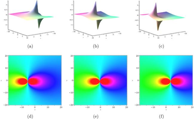
Figure 1. Three-dimensional plots and density plots of ( |
Case 24 ) has the following form9 ) into equation (2 ), we obtain
$\begin{eqnarray}\begin{array}{l}{a}_{1}=0,{a}_{2}={a}_{2},{a}_{3}=0,{a}_{4}={a}_{4},{a}_{5}={a}_{5},\\ {a}_{6}=0,{a}_{7}=-\displaystyle \frac{\alpha {a}_{5}}{4},{a}_{8}={a}_{8},{a}_{9}={a}_{9},\end{array}\end{eqnarray}$
where α, a2, a4, a5, a8, a9 are real free parameters. The lump solution of a positive quadratic function equation ( $\begin{eqnarray}\begin{array}{rcl}{f}_{2} & = & {\left({a}_{2}y+{a}_{4}\right)}^{2}\\ & & +\,{\left({a}_{5}x-\displaystyle \frac{\alpha {a}_{5}}{4}t+{a}_{8}\right)}^{2}+{a}_{9},\end{array}\end{eqnarray}$
then, substituting equation ( $\begin{eqnarray}{u}_{2}=\displaystyle \frac{2{a}_{5}\left({a}_{5}x-\tfrac{\alpha {a}_{5}}{4}t+{a}_{8}\right)}{{\left({a}_{2}y+{a}_{4}\right)}^{2}+{\left({a}_{5}x-\tfrac{\alpha {a}_{5}}{4}t+{a}_{8}\right)}^{2}+{a}_{9}}.\end{eqnarray}$
Figure 2 gives the plots of (10 ) and its density plots with the parameters α = 1, a2 = −2, a4 = −1, a5 = 0.4, a8 = 2, a9 = 1 when t = −10, 0, 10. By comparing figure 1 and figure 2, it can be seen that their shapes are similar, but by comparing the density diagram, the influence range of the solution formed under the figure 2 parameter presents a circle, while that of the solution formed under figure 2 parameter presents an ellipse.

Figure 2. Three-dimensional plots and density plots of ( |
3. Lump-type solution
In this section, we will talk about the lump-type solutions of the (2+1)-dimensional dissipative AKNS equation, which has many interesting phenomena. And we will explore three kinds of solutions, including lump-periodic solutions, lump-kink solutions, and lump-soliton solutions.
3.1. Lump-periodic solution
In this section, we will discuss the lump-periodic solution. We assume that the form of solution is11 ) into (3 ), then we solve the algebraic system of coefficients, we can obtain solutions for the following two cases
$\begin{eqnarray}\begin{array}{l}f={\left({b}_{1}x+{b}_{2}y+{b}_{3}t+{b}_{4}\right)}^{2}\\ +\,{b}_{5}\cos ({\theta }_{1})+{b}_{6}.\end{array}\end{eqnarray}$
θ1 = k1x + k2y + k3t + k4, taking (Case 112 ) into equation (11 ), we have13 ) into equation (2 ), we obtain
$\begin{eqnarray}\begin{array}{l}{b}_{1}={b}_{1},{b}_{2}=0,{b}_{3}=-\displaystyle \frac{\alpha {b}_{1}}{4},{b}_{4}={b}_{4},{b}_{5}={b}_{5},\\ {b}_{6}={b}_{6},{k}_{1}=0,{k}_{2}={k}_{2},{k}_{3}=0,{k}_{4}={k}_{4},\end{array}\end{eqnarray}$
where α, b1, b4, b5, b6, k2, k4 are real free parameters. Substituting equation ( $\begin{eqnarray}\begin{array}{rcl}{f}_{1} & = & {\left({b}_{1}x-\displaystyle \frac{\alpha {b}_{1}}{4}t+{b}_{4}\right)}^{2}\\ & & +\,{b}_{5}\cos \left({k}_{2}y+{k}_{4}\right)+{b}_{6},\end{array}\end{eqnarray}$
then, substituting equation ( $\begin{eqnarray}{u}_{1}=\displaystyle \frac{2{b}_{1}\left({b}_{1}x-\tfrac{\alpha {b}_{1}}{4}t+{b}_{4}\right)}{{\left({b}_{1}x-\tfrac{\alpha {b}_{1}}{4}t+{b}_{4}\right)}^{2}+{b}_{5}\cos ({k}_{2}y+{k}_{4})+{b}_{6}}.\end{eqnarray}$
Figure 3 gives the plots of (14 ) and its density plots with the parameters α = 2, b1 = 1, b4 = 2, b5 = − 2, b6 = 2, k2 = 1, k4 = 2 when t = −20, 0, 20. We notice that the lump solution appears periodically and only shifts along the x axis over time.

Figure 3. Three-dimensional plots and density plots of ( |
Case 215 ) into equation (11 ), we have16 ) into equation (2 ), we obtain
$\begin{eqnarray}\begin{array}{l}{b}_{1}=0,{b}_{2}=\displaystyle \frac{4{b}_{3}}{{k}_{1}^{2}},{b}_{3}={b}_{3},\\ {b}_{4}={b}_{4},{b}_{5}={b}_{5},\\ {b}_{6}={b}_{6},{k}_{1}={k}_{1},{k}_{2}=0,\\ {k}_{3}=-\displaystyle \frac{\alpha {k}_{1}}{4},{k}_{4}={k}_{4},\end{array}\end{eqnarray}$
where α, b3, b4, b5, b6, k1, k4 are real free parameters. Substituting equation ( $\begin{eqnarray}\begin{array}{rcl}{f}_{2} & = & {\left(\displaystyle \frac{4{b}_{3}}{{k}_{1}^{2}}y+{b}_{3}t+{b}_{4}\right)}^{2}\\ & & +\,{b}_{5}\cos \left({k}_{1}x-\displaystyle \frac{\alpha {k}_{1}}{4}t+{k}_{4}\right)+{b}_{6},\end{array}\end{eqnarray}$
then, substituting equation ( $\begin{eqnarray}{u}_{2}=\displaystyle \frac{-{k}_{1}{b}_{5}\sin \left({k}_{1}x-\tfrac{\alpha {k}_{1}}{4}t+{k}_{4}\right)}{{\left(\tfrac{4{b}_{3}}{{k}_{1}^{2}}y+{b}_{3}t+{b}_{4}\right)}^{2}+{b}_{5}\cos ({k}_{1}x-\tfrac{\alpha {k}_{1}}{4}t+{k}_{4})+{b}_{6}}.\end{eqnarray}$
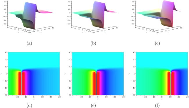
Figure 4 gives the plots of (17 ) and its density plots with the parameters α = 2, b3 = 0.5, b4 = 0.2, b5 = −1, b6 = 1.2, k1 = 1, k4 = 1 when t = −30, 0, 30. We notice that the lump solution appears periodically and only shifts along the y axis over time.

Figure 4. Three-dimensional plots and density plots of ( |
3.2. Lump-kink solution
In this section, we assume that the (2+1)-dimensional dissipative AKNS equation has a lump-kink solution and assume that the test function is:18 ) into (3 ), then we solve for an algebraic system of coefficients, we can obtain solutions for the following two cases.
$\begin{eqnarray}\begin{array}{rcl}f & = & {\left({c}_{1}x+{c}_{2}y+{c}_{3}t+{c}_{4}\right)}^{2}\\ & & +\,{c}_{5}\sinh ({\theta }_{2})+{c}_{6}.\end{array}\end{eqnarray}$
θ2 = w1x + w2y + w3t + w4, taking (Case 119 ) into equation (18 ), we have20 ) into equation (2 ), we obtain
$\begin{eqnarray}\begin{array}{l}{c}_{1}={c}_{1},{c}_{2}=0,{c}_{3}=-\displaystyle \frac{\alpha {c}_{1}}{4},\\ {c}_{4}={c}_{4},{c}_{5}={c}_{5},\\ {c}_{6}={c}_{6},{w}_{1}=0,{w}_{2}={w}_{2},\\ {w}_{3}=0,{w}_{4}={w}_{4},\end{array}\end{eqnarray}$
where αc1, c4, c5, c6, w2, w4 are real free parameters. Substituting equation ( $\begin{eqnarray}\begin{array}{l}{f}_{1}={\left({c}_{1}x-\displaystyle \frac{\alpha {c}_{1}}{4}t+{c}_{4}\right)}^{2}\\ +\,{c}_{5}\sinh ({w}_{2}y+{w}_{4})+{c}_{6},\end{array}\end{eqnarray}$
then, substituting equation ( $\begin{eqnarray}{u}_{1}=\displaystyle \frac{2{c}_{1}\left({c}_{1}x-\tfrac{\alpha {c}_{1}}{4}t+{c}_{4}\right)}{{\left({c}_{1}x-\tfrac{\alpha {c}_{1}}{4}t+{c}_{4}\right)}^{2}+{c}_{5}\sin h({w}_{2}y+{w}_{4})+{c}_{6}}.\end{eqnarray}$
The plots of (21 ) and its density plots with the parameters α = 3, c1 = 1, c4 = −3, c5 = 2, c6 = 1, w2 = 2, w4 = 1 when t = −5, 0, 5 are given in figure 5. According to the density diagram, we can see that kink occurs in the interaction solution, and this phenomenon only shifts in the horizontal direction over time, but its shape does not change.
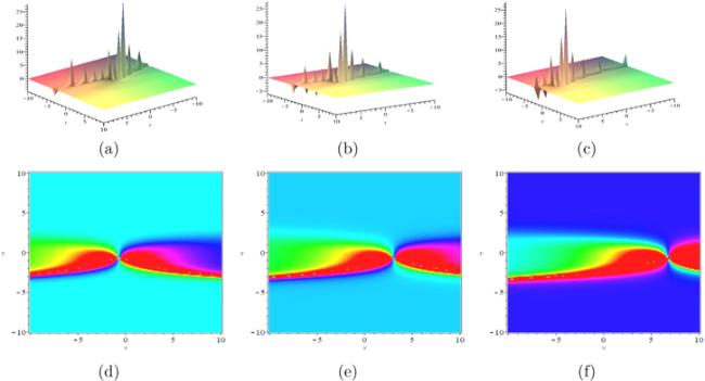
Figure 5. Three-dimensional plots and density plots of ( |
Case 222 ) into equation (18 ), we have23 ) into equation (2 ), we obtain
$\begin{eqnarray}\begin{array}{l}{c}_{1}=0,{c}_{2}=-\displaystyle \frac{4{c}_{3}}{{w}_{1}^{2}},{c}_{3}={c}_{3},\\ {c}_{4}={c}_{4},{c}_{5}={c}_{5},\\ {c}_{6}={c}_{6},{w}_{1}={w}_{1},{w}_{2}=0,\\ {w}_{3}=-\displaystyle \frac{\alpha {w}_{1}}{4},{w}_{4}={w}_{4},\end{array}\end{eqnarray}$
where α, c3, c4, c5, c6, w1, w4 are real free parameters. Substituting equation ( $\begin{eqnarray}\begin{array}{rcl}{f}_{2} & = & {\left(-\displaystyle \frac{4{c}_{3}}{{w}_{1}^{2}}y+{c}_{3}t+{c}_{4}\right)}^{2}\\ & & +\,{c}_{5}\sinh ({w}_{1}x-\displaystyle \frac{\alpha {w}_{1}}{4}t+{w}_{4})+{c}_{6},\end{array}\end{eqnarray}$
then, substituting equation ( $\begin{eqnarray}{u}_{2}=\displaystyle \frac{{w}_{1}{c}_{5}\cos h({w}_{1}x-\tfrac{\alpha {w}_{1}}{4}t+{w}_{4})}{{\left(-\tfrac{4{c}_{3}}{{w}_{1}^{2}}y+{c}_{3}t+{c}_{4}\right)}^{2}+{c}_{5}\sin h({w}_{1}x-\tfrac{\alpha {w}_{1}}{4}t+{w}_{4})+{c}_{6}}.\end{eqnarray}$
Figure 6 gives the plots of (24 ) and its density plots with the parameters $\alpha =1,{c}_{3}=\tfrac{5}{3}$, c4 = −1, c5 = 1, c6 = 1.5, ${w}_{1}=\tfrac{4}{3},{w}_{4}=-1$ when t = −10, 0, 9. As in case 1, the interaction also kink.
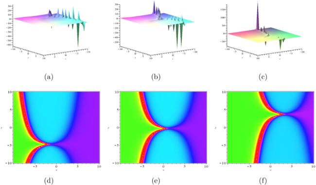
Figure 6. Three-dimensional plots and density plots of ( |
3.3. Lump-soliton solution
In this section, we will discuss the interaction between lump solution and soliton solution. We assume that the form of solution is25 ) into (3 ), then we solve for an algebraic system of coefficients, we can obtain solutions for the following two cases
$\begin{eqnarray}f={\left({d}_{1}x+{d}_{2}y+{d}_{3}t+{d}_{4}\right)}^{2}+{d}_{5}{e}^{{\theta }_{3}}+{d}_{6}.\end{eqnarray}$
θ3 = r1x + r2y + r3t + r4, taking (Case 125 ) has the following form:
$\begin{eqnarray}\begin{array}{l}{d}_{1}=0,{d}_{2}=-\displaystyle \frac{4{d}_{3}}{{r}_{1}^{2}},{d}_{3}={d}_{3},\\ {d}_{4}={d}_{4},{d}_{5}={d}_{5},\\ {d}_{6}={d}_{6},{r}_{1}={r}_{1},{r}_{2}=-\displaystyle \frac{\alpha {r}_{1}+4{r}_{3}}{{r}_{1}^{2}},\\ {r}_{3}={r}_{3},{r}_{4}={r}_{4},\end{array}\end{eqnarray}$
where α, d3, d4, d5, d6, r1, r3, r4 are real free parameters. Thus, the test function ( $\begin{eqnarray}\begin{array}{rcl}{f}_{1} & = & {\left(-\displaystyle \frac{4{d}_{3}}{{r}_{1}^{2}}y+{d}_{3}t+{d}_{4}\right)}^{2}\\ & & +\,{d}_{5}{{\rm{e}}}^{{r}_{1}x-\tfrac{\alpha {r}_{1}+4{r}_{3}}{{r}_{1}^{2}}y+{r}_{3}t+{r}_{4}}+{d}_{6},\end{array}\end{eqnarray}$
Under the condition of (27 ), the form of (2 ) is
$\begin{eqnarray}{u}_{1}=\displaystyle \frac{{r}_{1}{d}_{5}{{\rm{e}}}^{{r}_{1}x-\tfrac{\alpha {r}_{1}+4{r}_{3}}{{r}_{1}^{2}}y+{r}_{3}t+{r}_{4}}}{{\left(-\tfrac{4{d}_{3}}{{r}_{1}^{2}}y+{d}_{3}t+{d}_{4}\right)}^{2}+{d}_{5}{{\rm{e}}}^{{r}_{1}x-\tfrac{\alpha {r}_{1}+4{r}_{3}}{{r}_{1}^{2}}y+{r}_{3}t+{r}_{4}}+{d}_{6}}.\end{eqnarray}$
With the parameter α = 1.2, d3 = 1, d4 = 1.2, d5 = 1.5, d6 = 5, r1 = −1, r3 = 0.5, r4 = 2 when t = −20, 0, 20, the 3d plots and density plots are shown in figure 7. It can be seen that the interaction between soliton (kink-like) and lump does not change under the influence of time, and only moves in the horizontal direction.
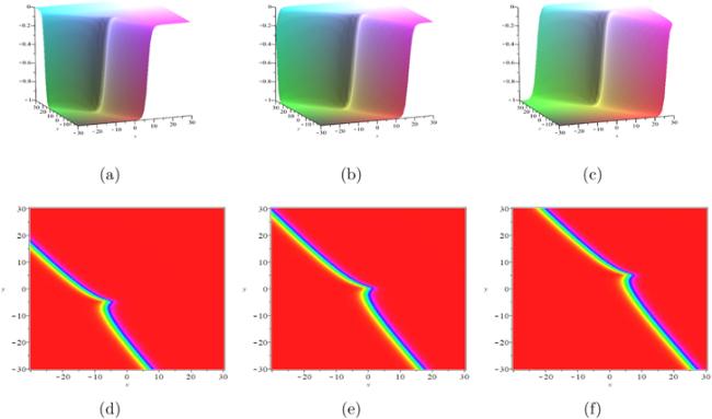
Figure 7. Three-dimensional plots and density plots of ( |
Case 2
$\begin{eqnarray}\begin{array}{l}{d}_{1}={d}_{1},{d}_{2}=0,{d}_{3}=-\displaystyle \frac{\alpha {d}_{1}}{4},\\ {d}_{4}={d}_{4},{d}_{5}={d}_{5},\\ {d}_{6}={d}_{6},{r}_{1}=0,{r}_{2}={r}_{2},\\ {r}_{3}=0,{r}_{4}={r}_{4},\end{array}\end{eqnarray}$
where α, d1, d4, d5, d6, r2, r4 are real free parameters.Under the condition of (29 ), (25 ) becomes30 ) into equation (2 ), we obtain
$\begin{eqnarray}\begin{array}{rcl}{f}_{2} & = & {\left({d}_{1}x-\displaystyle \frac{\alpha {d}_{1}}{4}t+{d}_{4}\right)}^{2}\\ & & +\,{d}_{5}{e}^{{r}_{2}y+{r}_{4}}+{d}_{6},\end{array}\end{eqnarray}$
then, substituting equation ( $\begin{eqnarray}{u}_{2}=\displaystyle \frac{2{d}_{1}\left({d}_{1}x-\tfrac{\alpha {d}_{1}}{4}t+{d}_{4}\right)}{{\left({d}_{1}x-\tfrac{\alpha {d}_{1}}{4}t+{d}_{4}\right)}^{2}+{d}_{5}{e}^{{r}_{2}y+{r}_{4}}+{d}_{6}}.\end{eqnarray}$
Figure 8 gives the plots of (31 ) and its density plots with the parameters α = 1, d1 = 1, d4 = 2, d5 = 1.5, d6 = 2, r2 = 1, r4 = −2 when t = −50, 0, 50.
Figure 8. Three-dimensional plots and density plots of ( |
4. Conclusions
In this paper, we study the (2+1)-dimensional dissipative AKNS equation. In view of [52], we obtained the lump solution and lump-type solution of the (2+1)-dimensional dissipative AKNS equation by assuming different forms of solution. By taking different parameters, we get different forms of the solution. Using Maple software, we draw three-dimensional images of the equation (1 ), and we find that the forms of the solution are very interesting. The lump solution will move in a corresponding position as time changes. Compared with the methods in [36, 37, 39, 45], we solve the exact solution of the (2+1)-dimensional dissipative AKNS equation by using the test function method, and we get the different existence states of the solution. For example, the lump-soliton solution is obtained by the combination of a lump solution and a soliton (kink-like) solution. The lump-soliton (kink-like) solution of equation (1 ) has not been studied by our predecessors. This undoubtedly enriches the physical behavior of the (2+1)-dimensional dissipative AKNS equation.
We give four kinds of test functions and obtain different states of the solutions. In fact, there are still many forms of test functions, please refer to [22, 28–30]. Of course, there are still many forms worth exploring for solutions of the (2+1)-dimensional dissipative AKNS equation. For example, we can get the D’alembert solution u = U(By + Ct + D) and u = U( − 4Cx + Ct + D) where B, C, D are auxiliary constants and U is an auxiliary function. In this paper, we only provide solutions of limited forms. There is also a lot of interesting work on exact solutions [53–56]. It is hoped that our results will be helpful to enrich the dynamic behavior of nonlinear evolution equations.