


1. Introduction
As is well known, lots of efficient methods have been available for seeking soliton solutions, including inverse scattering transform [1, 2], the RH approach [3–7], Darboux transform [8–10], ${\rm{B}}\ddot{{\rm{a}}}$cklund transform [11] and Hirota bilinear method [12]. Among the various methods, the RH approach has proved very powerful in deriving soliton solutions for many completely integrable equations. In fact, the RH approach is a special nonlinear mapping between the group of potentials and the relevant spectral dates. In recent years, a variety of excellent works have been achieved by RH approach, such as generalized Sasa-Satsuma equation [13], matrix modified Korteweg-de Vries equation [14], nonlinear Schrödinger equation [15] and nonlocal reverse-time nonlinear Schrödinger equation [16] etc.
At present, we consider the coupled Hirota equations [17]:2 ) is reduced to the nonlinear Schrödinger equation [19], which describes soliton propagation in nonlinear dispersive science. When a = 0, b = 1, equation (2 ) is reduced to the modified Korteweg-de Vries equation [20] which is also very representative. As we all know, equation (2 ) is a well studied nonlinear integrable system and serves as a classical model to describe a variety of nonlinear phenomena in many fields, such as optical fibers, electric communication and engineering fields. Zhang et al investigated the soliton solutions with nonzero boundary conditions [21], and Ankiewicz et al discussed the rogue waves and rational solutions of equation (2 ) in [22]. On the other hand, Guo et al studied the long-time asymptotic behavior of the solution of the Hirota equation by means of the nonlinear steepest descent method [23]. Recently, Xu et al obtained the explicit formulas of arbitrary-order multi-pole solutions of the Hirota equation via Darboux transformation and some limit techniques, at the same time, they studied the asymptotic behavior and the soliton interactions of the double- and triple-pole solutions [24]. In addition, other important results of the Hirota equation have been obtained in [25–28].
$\begin{eqnarray}{\rm{i}}{q}_{t}+a(-2{q}^{2}r+{q}_{{xx}})+{\rm{i}}b({q}_{{xxx}}-6{{qrq}}_{x})=0,\end{eqnarray}$
$\begin{eqnarray}{\rm{i}}{r}_{t}+a(2{r}^{2}q-{r}_{{xx}})+{\rm{i}}b({r}_{{xxx}}-6{{qrr}}_{x})=0,\end{eqnarray}$
where q(x, t) and r(x, t) are both the complex valued functions associated with the real variables x and t. Then a = a1 + ia2 and b = b1 + ib2, a1, a2, b1, b2 are real constants. It leads to the Hirota equation [18] which Hirota introduced for the first time in 1973 $\begin{eqnarray}{\rm{i}}{q}_{t}+a(2| q{| }^{2}q+{q}_{{xx}})+{\rm{i}}b({q}_{{xxx}}+6| q{| }^{2}{q}_{x})=0,\end{eqnarray}$
by the reduction r(x, t) = −q*(x, t), and * is the complex conjugate. When a = 1, b = 0, equation (In recent years, the nonlocal nonlinear integrable evolution equations [29–31] have been proposed and investigated by many researchers. In our present work, we are concerned with the nonlocal Hirota equations which have been studied in various methods [32, 33]. Furthermore, it is also meaningful to find the symmetries and analytic properties of the nonlocal Hirota equations. Now let us consider the following reductions r(x, t) = q*(ε1x, ε2t), where real constants ${\epsilon }_{1}^{2}={\epsilon }_{2}^{2}=1,$ special cases of equations (1 ) can be shown
| • | If a1 = b1 = 0, ε1 = 1 and ε2 = −1, equation ( $\begin{eqnarray}\begin{array}{l}{\rm{i}}{q}_{t}+a(-2{q}^{2}{q}^{* }(x,-t)+{q}_{{xx}})\\ \quad +{\rm{i}}b({q}_{{xxx}}-6{{qq}}^{* }(x,-t){q}_{x})=0.\end{array}\end{eqnarray}$ |
| • | If a2 = b1 = 0, ε1 = − 1 and ε2 = 1, equation ( $\begin{eqnarray}\begin{array}{l}{\rm{i}}{q}_{t}+a(-2{q}^{2}{q}^{* }(-x,t)+{q}_{{xx}})\\ \quad +{\rm{i}}b({q}_{{xxx}}-6{{qq}}^{* }(-x,t){q}_{x})=0.\end{array}\end{eqnarray}$ |
| • | If a1 = b2 = 0, ε1 = −1 and ε2 = −1, one obtains the reverse-spacetime nonlocal Hirota equation: $\begin{eqnarray}\begin{array}{l}{\rm{i}}{q}_{t}+a(-2{q}^{2}{q}^{* }(-x,-t)+{q}_{{xx}})\\ \quad +{\rm{i}}b({q}_{{xxx}}-6{{qq}}^{* }(-x,-t){q}_{x})=0.\end{array}\end{eqnarray}$ |
The rest of this paper is as follows. In section 2 , we analyze the analyticity of matrix eigenfunctions by introducing the equivalent spectral problem and establish the RH problem on the real-λ line. In section 3 , three cases of the nonlocal Hirota equations are discussed, respectively, then the multi-soliton solutions of the nonlocal Hirota equations are derived from a specific RH problem. Finally, a concise summary of this paper will be presented in section 4 .
2. The Riemann–Hilbert problem
The Lax pair for the equation (1 ) can be written as follows
$\begin{eqnarray}{{\rm{\Phi }}}_{x}=M{\rm{\Phi }}=(-{\rm{i}}\lambda {\sigma }_{3}+U){\rm{\Phi }},\end{eqnarray}$
$\begin{eqnarray}{{\rm{\Phi }}}_{t}=N{\rm{\Phi }}=[-(4b{\rm{i}}{\lambda }^{3}+2a{\rm{i}}{\lambda }^{2}){\sigma }_{3}+V]{\rm{\Phi }},\end{eqnarray}$
with
$\begin{eqnarray*}{\sigma }_{3}=\left(\begin{array}{cc}1 & 0\\ 0 & -1\end{array}\right),U=\left(\begin{array}{cc}0 & q(x,t)\\ r(x,t) & 0\end{array}\right),\end{eqnarray*}$
$\begin{eqnarray*}\begin{array}{rcl}V & = & {\lambda }^{3}\left(\begin{array}{cc}-4b{\rm{i}} & 0\\ 0 & 4b{\rm{i}}\end{array}\right)+{\lambda }^{2}\left(\begin{array}{cc}-2a{\rm{i}} & 4{bq}\\ 4{br} & 2a{\rm{i}}\end{array}\right)\\ & & +\,\lambda \left(\begin{array}{cc}-2b{\rm{i}}{qr} & 2b{\rm{i}}{q}_{x}+2{aq}\\ -2b{\rm{i}}{r}_{x}+2{ar} & 2b{\rm{i}}{qr}\end{array}\right)\\ & & +\,\left(\begin{array}{cc}-a{\rm{i}}{qr}+b({{rq}}_{x}-{{qr}}_{x}) & {\rm{i}}{{aq}}_{x}-b({q}_{{xx}}-2{q}^{2}r)\\ -{\rm{i}}{{ar}}_{x}+b(-{r}_{{xx}}+2{{qr}}^{2}) & {\rm{i}}{aqr}-b({{rq}}_{x}-{{qr}}_{x})\end{array}\right),\end{array}\end{eqnarray*}$
where ${\rm{\Phi }}(x,t,\lambda )={\left({\phi }_{1}(x,t,\lambda ),{\phi }_{2}(x,t,\lambda )\right)}^{{\rm{T}}}$ is the spectral function. M and N satisfy the zero curvature equation Mt − Nx + [M, N] = 0.
In order to proceed to the later research work, one can introduce the Jost solution from reading as
$\begin{eqnarray}{\rm{\Phi }}(x,t,\lambda )\sim {{\rm{e}}}^{-{\rm{i}}\lambda {\sigma }_{3}x-(4b{\rm{i}}{\lambda }^{3}+2a{\rm{i}}{\lambda }^{2}){\sigma }_{3}t},\quad | x| \to \infty .\end{eqnarray}$
Hence, let $\kappa (x,t,\lambda )={\rm{\Phi }}(x,t,k){{\rm{e}}}^{{\rm{i}}\lambda {\sigma }_{3}x+(4b{\rm{i}}{\lambda }^{3}+2a{\rm{i}}{\lambda }^{2}){\sigma }_{3}t}$ be a new matrix-valued spectral function, and $\begin{eqnarray}\kappa (x,t,\lambda )\to {\mathbb{I}},\quad | x| \to \infty ,\end{eqnarray}$
where ${\mathbb{I}}$ is the 2 × 2 identity matrix. Therefore, we obtain the equivalent spectral problem in the following form
$\begin{eqnarray}{\kappa }_{x}+{\rm{i}}\lambda [{\sigma }_{3},\kappa ]=U\kappa ,\end{eqnarray}$
$\begin{eqnarray}{\kappa }_{t}+(4b{\rm{i}}{\lambda }^{3}+2a{\rm{i}}{\lambda }^{2})[{\sigma }_{3},\kappa ]=V\kappa ,\end{eqnarray}$
where [σ3, κ] = σ3κ − κσ3. In order to perform spectral analysis conveniently, the eigenfunctions κ± are accurately expressed via the Volterra integral equations
$\begin{eqnarray}{\kappa }_{-}(x,\lambda )={\mathbb{I}}+{\int }_{-\infty }^{x}{{\rm{e}}}^{-{\rm{i}}\lambda (x-y){\sigma }_{3}}U{\kappa }_{-}(y,\lambda ){{\rm{e}}}^{{\rm{i}}\lambda (x-y){\sigma }_{3}}{\rm{d}}{y},\end{eqnarray}$
$\begin{eqnarray}{\kappa }_{+}(x,\lambda )={\mathbb{I}}-{\int }_{x}^{+\infty }{{\rm{e}}}^{-{\rm{i}}\lambda (x-y){\sigma }_{3}}U{\kappa }_{+}(y,\lambda ){{\rm{e}}}^{{\rm{i}}\lambda (x-y){\sigma }_{3}}{\rm{d}}{y}.\end{eqnarray}$
The matrix Jost solutions can be expressed in a collection of the following columns,
$\begin{eqnarray}{\kappa }_{-}=({[{\kappa }_{-}]}_{1},{[{\kappa }_{-}]}_{2}),\quad {\kappa }_{+}=({[{\kappa }_{+}]}_{1},{[{\kappa }_{+}]}_{2}).\end{eqnarray}$
Therefore, it can be proved that ${[{\kappa }_{-}]}_{1}$ and ${[{\kappa }_{+}]}_{2}$ are analytic in ${{\mathbb{C}}}^{+}$, ${[{\kappa }_{+}]}_{1}$ and ${[{\kappa }_{-}]}_{2}$ are analytic in ${{\mathbb{C}}}^{-}$, where
$\begin{eqnarray*}\begin{array}{rcl}{{\mathbb{C}}}^{-} & = & \{\lambda \in {\mathbb{C}}| \mathrm{Im}(\lambda )\lt 0\},\\ {{\mathbb{C}}}^{+} & = & \{\lambda \in {\mathbb{C}}| \mathrm{Im}(\lambda )\gt 0\}.\end{array}\end{eqnarray*}$
Considering the spectral problem of equations (9 ), there exists two different matrix solutions
$\begin{eqnarray}{{\rm{\Phi }}}_{-}={\kappa }_{-}{{\rm{e}}}^{-{\rm{i}}\lambda {\sigma }_{3}x},\quad {{\rm{\Phi }}}_{+}={\kappa }_{+}{{\rm{e}}}^{-{\rm{i}}\lambda {\sigma }_{3}x},\end{eqnarray}$
linearly associated with a 2 × 2 scattering matrix S(λ)
$\begin{eqnarray}{\kappa }_{-}={\kappa }_{+}{{\rm{e}}}^{-{\rm{i}}\lambda {\sigma }_{3}x}S(\lambda ){{\rm{e}}}^{{\rm{i}}\lambda {\sigma }_{3}x}.\end{eqnarray}$
Based on Abel’s formula and ${tr}(U)=0$, it can be derived that κ− and κ+ are independent of x. Then, it yields
$\begin{eqnarray}\det \,{\kappa }_{-}=1,\quad \det \,{\kappa }_{+}=1.\end{eqnarray}$
According to the above results, combined with the asymptotic results: ${\kappa }_{\pm }\to {\mathbb{I}}$, as ∣x∣ → ∞ . We obtain the following result from equation (13 )
$\begin{eqnarray}\det \,S(\lambda )=1.\end{eqnarray}$
To develop associated RH problems, we adopt the spectral problem of adjoint matrix eigenfunctions. Notice that the inverse matrices ${\tilde{\kappa }}_{\pm }={\left({\kappa }_{\pm }\right)}^{-1}$, therefore, upon writing ${\left({\kappa }_{\pm }\right)}^{-1}$ as
$\begin{eqnarray}{\kappa }_{-}^{-1}=\left(\begin{array}{c}{\left[{\kappa }_{-}^{-1}\right]}_{1}\\ {\left[{\kappa }_{-}^{-1}\right]}_{2}\end{array}\right),\quad {\kappa }_{+}^{-1}=\left(\begin{array}{c}{\left[{\kappa }_{+}^{-1}\right]}_{1}\\ {\left[{\kappa }_{+}^{-1}\right]}_{2}\end{array}\right).\end{eqnarray}$
Furthermore, we know that ${[{\kappa }_{-}^{-1}]}_{2}$ and ${[{\kappa }_{+}^{-1}]}_{1}$ are analytic in ${{\mathbb{C}}}^{+}$, ${[{\kappa }_{-}^{-1}]}_{1}$ and ${[{\kappa }_{+}^{-1}]}_{2}$ are analytic in ${{\mathbb{C}}}^{-}$. From equation (13 ), the elements of S(λ) can be expressed
$\begin{eqnarray}\begin{array}{rcl}S(\lambda ) & = & {{\rm{e}}}^{{\rm{i}}\lambda {\sigma }_{3}x}{\kappa }_{+}^{-1}{\kappa }_{-}{{\rm{e}}}^{-{\rm{i}}\lambda {\sigma }_{3}x}\\ & = & {{\rm{e}}}^{{\rm{i}}\lambda {\sigma }_{3}x}\left(\begin{array}{cc}{[{\kappa }_{+}^{-1}]}_{1}{[{\kappa }_{-}]}_{1} & {[{\kappa }_{+}^{-1}]}_{1}{[{\kappa }_{-}]}_{2}\\ {\left[{\kappa }_{+}^{-1}\right]}_{2}{[{\kappa }_{-}]}_{1} & {\left[{\kappa }_{+}^{-1}\right]}_{2}{[{\kappa }_{-}]}_{2}\end{array}\right){{\rm{e}}}^{-{\rm{i}}\lambda {\sigma }_{3}x}\\ & = & \left(\begin{array}{cc}{s}_{11} & {s}_{12}\\ {s}_{21} & {s}_{22}\end{array}\right).\end{array}\end{eqnarray}$
It is obvious to infer that s11 is analytic in ${{\mathbb{C}}}^{+}$, and s22 is analytic in ${{\mathbb{C}}}^{-}$.
In order to construct the RH problem, we define the matrix solutions P+ and P− as follows
$\begin{eqnarray}{P}_{+}=({[{\kappa }_{-}]}_{1},{[{\kappa }_{+}]}_{2})={\kappa }_{-}{A}_{1}+{\kappa }_{+}{A}_{2},\end{eqnarray}$
$\begin{eqnarray}{P}_{-}=\left(\begin{array}{c}{\left[{\kappa }_{-}^{-1}\right]}_{1}\\ {\left[{\kappa }_{+}^{-1}\right]}_{2}\end{array}\right)={A}_{1}{\kappa }_{-}^{-1}+{A}_{2}{\kappa }_{+}^{-1},\end{eqnarray}$
where ${A}_{1}=\left(\begin{array}{cc}1 & 0\\ 0 & 0\end{array}\right)$ and ${A}_{2}=\left(\begin{array}{cc}0 & 0\\ 0 & 1\end{array}\right)$. Therefore, we easily obtain that ${P}_{+},{P}_{-}\to {\mathbb{I}}$ , as λ → ∞ .
Based on the above facts, the RH problem is established:
The jump matrix can be calculated as
| • | P+ is analytic in ${{\mathbb{C}}}^{+}$, P− is analytic in ${{\mathbb{C}}}^{-}$, |
| • | ${P}_{-}(x,t,\lambda ){P}_{+}(x,t,\lambda )=J(x,t,\lambda ),\quad \lambda \in {\mathbb{R}}$, |
| • | ${P}_{\pm }(x,t,\lambda )\to {\mathbb{I}}$ , as λ → ∞ . |
$\begin{eqnarray}J(x,t,\lambda )={{\rm{e}}}^{-{\rm{i}}\lambda {\sigma }_{3}x}\left(\begin{array}{cc}1 & {r}_{12}\\ {s}_{21} & 1\end{array}\right){{\rm{e}}}^{{\rm{i}}\lambda {\sigma }_{3}x},\end{eqnarray}$
and
$R(\lambda )=\left(\begin{array}{cc}{r}_{11} & {r}_{12}\\ {r}_{21} & {r}_{22}\end{array}\right)={S}^{-1}(\lambda )$, r11s11 + r12s21 = 1.
3. Multi-soliton solutions for the nonlocal Hirota equations
In this section, considering three nonlocal reductions, we solve the RH problem which corresponds to the reflectionless case and obtain multi-soliton solutions of the nonlocal Hirota equations.
3.1. Multi-soliton solutions of reverse-time nonlocal Hirota equation
According to the definition of P+, P− and the scattering relationship between κ+ and κ−, it yields
$\begin{eqnarray}\det \,{P}_{+}(x,\lambda )={s}_{11},\quad \lambda \in {{\mathbb{C}}}^{+},\end{eqnarray}$
$\begin{eqnarray}\det \,{P}_{-}(x,\lambda )={r}_{11},\quad \lambda \in {{\mathbb{C}}}^{-},\end{eqnarray}$
which shows that the zero structure of r11, s11 are the same as ${\rm{\det }}\,{P}_{-}(x,\lambda )$, ${\rm{\det }}\,{P}_{+}(x,\lambda )$. Because of the symmetry nonlocal relation U†(x, −t) = −σ3U(x, t)σ3, we have
$\begin{eqnarray}{\kappa }_{\pm }^{\dagger }(x,-t,{\lambda }^{* })={\sigma }_{3}{\kappa }_{\pm }^{-1}(x,t,\lambda ){\sigma }_{3}.\end{eqnarray}$
Here † denotes conjugate transpose, it can be obtained from equations (18 ) and (19 ) that
$\begin{eqnarray}{P}_{+}(x,-t,{\lambda }^{* })={\sigma }_{3}{P}_{-}(x,t,\lambda ){\sigma }_{3}.\end{eqnarray}$
According to equation (17 ), it yields
$\begin{eqnarray}{S}^{\dagger }({\lambda }^{* })={\sigma }_{3}{S}^{-1}(\lambda ){\sigma }_{3},\end{eqnarray}$
which implies the relationship
$\begin{eqnarray}{r}_{11}^{* }({\lambda }^{* })={s}_{11}(\lambda ).\end{eqnarray}$
This reveals that each zero ±λk of s11 corresponding to each zero $\pm {\lambda }_{k}^{* }$ of r11. Therefore, now we assume that there exists N simple zeros {λk}(1 ≤ k ≤ N) of s11 in ${{\mathbb{C}}}^{+}$, and exists N simple zeros $\{{\lambda }_{k}^{* }\}$ of r11 in ${{\mathbb{C}}}^{-}$, where
$\begin{eqnarray}{\lambda }_{k}^{* }={\lambda }_{k},\quad 1\leqslant k\leqslant N.\end{eqnarray}$
We define vk and ${v}_{k}^{* }$ to be nonzero column vectors and row vectors, respectively, which satisfy
$\begin{eqnarray}{P}_{+}({\lambda }_{k}){v}_{k}({\lambda }_{k})=0,\end{eqnarray}$
$\begin{eqnarray}{v}_{k}^{* }({\lambda }_{k}^{* }){P}_{-}({\lambda }_{k}^{* })=0.\end{eqnarray}$
Comparing the equations and taking the Hermitian conjugate of P+(λk)vk(λk) = 0, one can obtain
$\begin{eqnarray}{v}_{k}^{* }({\lambda }_{k}^{* })={v}_{k}^{\dagger }(\lambda ){\sigma }_{3}.\end{eqnarray}$
Solving equations (27 ) and utilizing Lax pair (9 ), we have
$\begin{eqnarray}{v}_{k}={{\rm{e}}}^{-{\theta }_{k}{\sigma }_{3}}{v}_{k,0},\end{eqnarray}$
$\begin{eqnarray}{v}_{k}^{* }={v}_{k,0}^{\dagger }{{\rm{e}}}^{-{\theta }_{k}^{* }(x,-t){\sigma }_{3}}{\sigma }_{3},\end{eqnarray}$
where ${v}_{k,0}={\left({\alpha }_{k},{\beta }_{k}\right)}^{{\rm{T}}}$ is a constant column vector and ${\theta }_{k}={\rm{i}}{\lambda }_{k}x+(4b{\rm{i}}{\lambda }_{k}^{3}+2a{\rm{i}}{\lambda }_{k}^{2})t\,(1\leqslant k\leqslant N)$.
As a matter of fact, J is a 2 × 2 identity matrix when the scattering coefficients s21 = s12 = 0. Then we can solve the RH problem, and the solutions to the RH problem are described by
$\begin{eqnarray}{P}_{+}(\lambda )={\mathbb{I}}-\sum _{k,j=1}^{N}\displaystyle \frac{{v}_{k}{v}_{j}^{* }{\left({M}^{-1}\right)}_{{kj}}}{\lambda -{\lambda }_{j}^{* }},\end{eqnarray}$
$\begin{eqnarray}{P}_{-}(\lambda )={\mathbb{I}}+\sum _{k,j=1}^{N}\displaystyle \frac{{v}_{k}{v}_{j}^{* }{\left({M}^{-1}\right)}_{{kj}}}{\lambda -{\lambda }_{k}^{* }},\end{eqnarray}$
where matrix $M={\left({m}_{{kj}}\right)}_{N\,\times \,N}$, we define its (k, j) element as follows
$\begin{eqnarray}{m}_{{kj}}=\displaystyle \frac{{v}_{k}^{* }{v}_{j}}{{\lambda }_{j}-{\lambda }_{k}^{* }},\quad 1\leqslant k,j\leqslant N.\end{eqnarray}$
At present, we are in a position to derive the multi-soliton solutions of the nonlocal Hirota equation. To this end, one can investigate P+ in (30 ) to Laurent expansion as
$\begin{eqnarray}{P}_{+}(\lambda )={\mathbb{I}}+{\lambda }^{-1}{P}_{+}^{(1)}+{\lambda }^{-2}{P}_{+}^{(2)}+o({\lambda }^{-3}),\quad \lambda \to \infty .\end{eqnarray}$
Then substituting equation (31 ) into P+,x + iλ[σ3, P+] = UP+ and equating the corresponding coefficients of the O(1) terms, we have
$\begin{eqnarray}U={\rm{i}}[{\sigma }_{3},{P}_{+}^{(1)}],\end{eqnarray}$
which reveals that $\begin{eqnarray}q(x,t)=2{\rm{i}}{\left({P}_{+}^{(1)}\right)}_{12},\end{eqnarray}$
$\begin{eqnarray}{q}^{* }(x,-t)=-2{\rm{i}}{\left({P}_{+}^{(1)}\right)}_{21},\end{eqnarray}$
where ${\left({P}_{+}^{(1)}\right)}_{12}$ is the (1, 2)-element of the matrix function ${P}_{+}^{(1)}$. Therefore, ${P}_{+}^{(1)}$ can be obtained by comparing corresponding elements $\begin{eqnarray}{P}_{+}^{(1)}=-\sum _{k,j=1}^{N}{v}_{k}{v}_{j}^{* }{\left({M}^{-1}\right)}_{{kj}}.\end{eqnarray}$
As a result, the multi-soliton solutions to the nonlocal Hirota equation can be expressed explicitly as
$\begin{eqnarray}q(x,t)=2{\rm{i}}\sum _{k,j=1}^{N}{\alpha }_{k}{\beta }_{j}^{* }{{\rm{e}}}^{-{\theta }_{k}-{\theta }_{j}^{* }(x,-t)}{\left({M}^{-1}\right)}_{{kj}},\end{eqnarray}$
where
${m}_{{kj}}=\tfrac{{\alpha }_{k}^{* }{\alpha }_{j}{{\rm{e}}}^{-{\theta }_{k}^{* }(x,-t)-{\theta }_{j}}-{\beta }_{k}^{* }{\beta }_{j}{{\rm{e}}}^{{\theta }_{k}^{* }(x,-t)+{\theta }_{j}}}{{\lambda }_{j}-{\lambda }_{k}^{* }}$ , 1 ≤ k, j ≤ N.
3.2. Multi-soliton solutions of reverse-space nonlocal Hirota equation
Compared with equation (3 ), there will be different symmetry relation to equation (4 ). Notice that U = U(x, t) satisfies the symmetry relation
$\begin{eqnarray}{U}^{* }(-x,t)=-{\sigma }_{1}^{-1}U(x,t){\sigma }_{1},\end{eqnarray}$
where ${\sigma }_{1}=\left(\begin{array}{cc}0 & 1\\ -1 & 0\end{array}\right)$. Under the circumstance, the relation of the matrix spectral functions κ± can be obtained
$\begin{eqnarray}{\kappa }_{\pm }(x,\lambda )={\sigma }_{1}^{-1}{\kappa }_{\mp }^{* }(-x,-{\lambda }^{* }){\sigma }_{1}.\end{eqnarray}$
According to the above relation and the definition of P±, then P− and P+ satisfy the following relations:
$\begin{eqnarray}{P}_{+}^{* }(-x,-{\lambda }^{* })={\sigma }_{1}{P}_{+}(x,\lambda ){\sigma }_{1}^{-1},\quad \lambda \in {{\mathbb{C}}}^{+},\end{eqnarray}$
$\begin{eqnarray}{P}_{-}^{* }(-x,-{\lambda }^{* })={\sigma }_{1}{P}_{-}(x,\lambda ){\sigma }_{1}^{-1},\quad \lambda \in {{\mathbb{C}}}^{-}.\end{eqnarray}$
Furthermore, the relationship of the scattering matrix and scattering data can be obtained:
$\begin{eqnarray}S(-{\lambda }^{* })={\sigma }_{1}{S}^{-1}(\lambda ){\sigma }_{1},\end{eqnarray}$
$\begin{eqnarray}{s}_{11}^{* }(-{\lambda }^{* })={r}_{22}(\lambda ),\quad {s}_{22}^{* }(-{\lambda }^{* })={r}_{11}(\lambda ).\end{eqnarray}$
Through the above results, the zero structure of the nonlocal Hirota equation can be given. Actually, from equations (39 ) we know that $\det \,{P}_{+}* (-x,-{\lambda }^{* })=\det \,{P}_{+}(x,\lambda )$, $\det \,{P}_{-}* (-x,-{\lambda }^{* })=\det \,{P}_{-}(x,\lambda )$. Thus, if λk is the zero of $\det \,{P}_{+}(x,\lambda )$, so is $-{\lambda }_{k}^{* }$. If ${\hat{\lambda }}_{k}$ is the zero of $\det \,{P}_{-}(x,\lambda )$, so is $-{\hat{\lambda }}_{k}^{* }$. Then, the zero structure of the nonlocal Hirota equation involves pairwise zeros $({\lambda }_{k},-{\lambda }_{k}^{* })$ and $({\hat{\lambda }}_{k},-{\hat{\lambda }}_{k}^{* })$.
The scattering data is needed to solve the RH problem including the continuous scattering dates {s12, s21} as well as the discrete scattering dates $\{{\lambda }_{k},{\hat{\lambda }}_{k},{v}_{k},{\hat{v}}_{k}\}$, in which vk and ${\hat{v}}_{k}$ are nonzero column vectors and row vectors, respectively, they satisfy
$\begin{eqnarray}{P}_{+}({\lambda }_{k}){v}_{k}({\lambda }_{k})=0,\end{eqnarray}$
$\begin{eqnarray}{\hat{v}}_{k}({\lambda }_{k}){P}_{-}({\hat{\lambda }}_{k})=0.\end{eqnarray}$
For the purpose of obtaining the explicit form of the vectors vk and ${\hat{v}}_{k}$, we calculate the derivatives of equations (42 ) with respect to x and t and find
$\begin{eqnarray}{v}_{k}=\left\{\begin{array}{ll}{{\rm{e}}}^{-{\theta }_{k}{\sigma }_{3}}{v}_{k,0},\quad & 1\leqslant k\leqslant N,\\ {\sigma }_{1}{{\rm{e}}}^{-{\theta }_{k-N}^{* }(-x,t){\sigma }_{3}}{v}_{k-N,0}^{* },\quad & N+1\leqslant k\leqslant 2N,\end{array}\right.\end{eqnarray}$
$\begin{eqnarray}{\hat{v}}_{k}=\left\{\begin{array}{ll}{\hat{v}}_{k,0}{{\rm{e}}}^{{\hat{\theta }}_{k}{\sigma }_{3}},\quad & 1\leqslant k\leqslant N,\\ {\hat{v}}_{k-N,0}^{* }{{\rm{e}}}^{{\hat{\theta }}_{k-N}^{* }(-x,t){\sigma }_{3}}{\sigma }_{1},\quad & N+1\leqslant k\leqslant 2N,\end{array}\right.\end{eqnarray}$
with ${\theta }_{k}={\rm{i}}{\lambda }_{k}x+(4b{\rm{i}}{\lambda }_{k}^{3}+2a{\rm{i}}{\lambda }_{k}^{2})t$, ${\hat{\theta }}_{k}={\rm{i}}\hat{{\lambda }_{k}}x+(4b{\rm{i}}{\hat{\lambda }}_{k}^{3}\,+2a{\rm{i}}{\hat{\lambda }}_{k}^{2})t$, ${v}_{k,0}={\left({\alpha }_{k},{\beta }_{k}\right)}^{T}$ and ${\hat{v}}_{k,0}=({\hat{\alpha }}_{k},{\hat{\beta }}_{k})$ are nonzero vectors.
Similar to section 3.1 , one can also introduce a 2N × 2N matrix M with entries ${m}_{{kj}}=\tfrac{{\hat{v}}_{k}{v}_{j}}{{\lambda }_{j}-{\hat{\lambda }}_{k}}\quad (1\leqslant k,j\leqslant 2N)$, and assuming that the inverse matrix of M exists, then the solution for the RH problem can be given by
$\begin{eqnarray}{P}^{+}(\lambda )={\mathbb{I}}-\sum _{k,j=1}^{2N}\displaystyle \frac{{v}_{k}{\hat{v}}_{j}^{* }{\left({M}^{-1}\right)}_{{kj}}}{\lambda -{\hat{\lambda }}_{j}},\end{eqnarray}$
$\begin{eqnarray}{P}^{-}(\lambda )={\mathbb{I}}+\sum _{k,j=1}^{2N}\displaystyle \frac{{v}_{k}{\hat{v}}_{j}^{* }{\left({M}^{-1}\right)}_{{kj}}}{\lambda -{\lambda }_{k}}.\end{eqnarray}$
We can also expand P+ as in section 3.1 and get the following formulas:
$\begin{eqnarray}q(x,t)=2i{\left({P}_{+}^{(1)}\right)}_{12},\end{eqnarray}$
$\begin{eqnarray}{q}^{* }(-x,t)=-2i{\left({P}_{+}^{(1)}\right)}_{21}.\end{eqnarray}$
Furthermore, from equations (44 ) we directly obtain
$\begin{eqnarray}{P}_{+}^{(1)}=-\sum _{k,j=1}^{2N}{v}_{k}{v}_{j}^{* }{\left({M}^{-1}\right)}_{{kj}}.\end{eqnarray}$
Therefore, the expression of 2N-soliton solutions to the nonlocal Hirota equation reads
$\begin{eqnarray}\begin{array}{rcl}q(x,t) & = & -2{\rm{i}}\displaystyle \sum _{k=1}^{N}\displaystyle \sum _{j=1}^{N}{\alpha }_{k}{\hat{\beta }}_{j}{{\rm{e}}}^{-{\theta }_{k}-{\hat{\theta }}_{j}}{\left({M}^{-1}\right)}_{{kj}}\\ & & -\,2{\rm{i}}\displaystyle \sum _{k=1}^{N}\displaystyle \sum _{j=N+1}^{2N}{\alpha }_{k}{\hat{\alpha }}_{j-N}^{* }{{\rm{e}}}^{-{\theta }_{k}+{\hat{\theta }}_{j-N}^{* }(-x,t)}{\left({M}^{-1}\right)}_{{kj}}\\ & & -\,2{\rm{i}}\displaystyle \sum _{k=N+1}^{2N}\displaystyle \sum _{j=1}^{N}{\beta }_{k-N}^{* }{\hat{\beta }}_{j}{{\rm{e}}}^{{\theta }_{k-N}^{* }(-x,t)-{\hat{\theta }}_{j}}{\left({M}^{-1}\right)}_{{kj}}\\ & & -\,2{\rm{i}}\displaystyle \sum _{k=N+1}^{2N}\displaystyle \sum _{j=N+1}^{2N}{\beta }_{k-N}^{* }{\hat{\alpha }}_{j-N}^{* }{{\rm{e}}}^{{\theta }_{k-N}^{* }(-x,t)+{\hat{\theta }}_{j-N}^{* }(-x,t)}\\ & & \times \,{\left({M}^{-1}\right)}_{{kj}},\end{array}\end{eqnarray}$
with the matrix entries
$\begin{eqnarray*}{m}_{{kj}}=\left\{\begin{array}{ll}\displaystyle \frac{\alpha k{\hat{\alpha }}_{j}{{\rm{e}}}^{-{\hat{\theta }}_{k}-{\theta }_{j}}+{\hat{\beta }}_{k}{\beta }_{j}{{\rm{e}}}^{-{\hat{\theta }}_{k}+{\theta }_{j}}}{{\lambda }_{j}-{\hat{\lambda }}_{k}},\quad & 1\leqslant k,j\leqslant N,\\ \displaystyle \frac{{\hat{\alpha }}_{k}{\beta }_{j-N}^{* }{{\rm{e}}}^{-{\hat{\theta }}_{k}-{\theta }_{j-N}^{* }(-x,t)}-{\hat{\beta }}_{k}{\alpha }_{j-N}^{* }{{\rm{e}}}^{-{\hat{\theta }}_{k}-{\theta }_{j-N}^{* }(-x,t)}}{-{\lambda }_{j-N}^{* }-{\hat{\lambda }}_{k}},\quad & 1\leqslant k\leqslant N,N+1\leqslant j\leqslant 2N,\\ \displaystyle \frac{-{\hat{\beta }}_{k-N}^{* }{\alpha }_{j}{{\rm{e}}}^{-{\hat{\theta }}_{k-N}^{* }(-x,t)-{\theta }_{j}}+{\hat{\beta }}_{k-N}^{* }{\beta }_{j}{{\rm{e}}}^{{\hat{\theta }}_{k-N}^{* }(-x,t)+{\theta }_{j}}}{{\lambda }_{j}+{\hat{\lambda }}_{k-N}^{* }},\quad & N+1\leqslant k\leqslant 2N,1\leqslant j\leqslant N,\\ \displaystyle \frac{-{\hat{\beta }}_{k-N}^{* }{\beta }_{j-N}^{* }{{\rm{e}}}^{-{\hat{\theta }}_{k-N}^{* }(-x,t)+{\theta }_{j-N}^{* }(-x,t)}-{\hat{\alpha }}_{k-N}^{* }{\alpha }_{j-N}^{* }{{\rm{e}}}^{{\hat{\theta }}_{k-N}^{* }(-x,t)+{\theta }_{j-N}^{* }(-x,t)}}{-{\lambda }_{j-N}^{* }+{\hat{\lambda }}_{k-N}^{* }},\quad & N+1\leqslant k\leqslant 2N,N+1\leqslant j\leqslant 2N.\end{array}\right.\end{eqnarray*}$
3.3. Multi-soliton solutions of reverse-spacetime nonlocal Hirota equation
We assume that $\det \,{P}_{+}(x,\lambda )$ and $\det \,{P}_{-}(x,\lambda )$ possess certain zeros ${\lambda }_{k}\in {{\mathbb{C}}}^{+}$ and ${\lambda }_{k}\in {{\mathbb{C}}}^{-}(1\leqslant k\leqslant 2N$) when this RH problem is non-regular, where 2N is the number of these zeros. According to the expressions of P+ and P− mentioned above, one can easily find that
$\begin{eqnarray}\det \,{P}_{+}(x,\lambda )={s}_{11},\quad \lambda \in {{\mathbb{C}}}^{+},\end{eqnarray}$
$\begin{eqnarray}\det \,{P}_{-}(x,\lambda )={r}_{11},\quad \lambda \in {{\mathbb{C}}}^{-}.\end{eqnarray}$
Combining the symmetry relationships ${U}^{* }(-x,-t)\,=-{\sigma }_{1}^{-1}U(x,t){\sigma }_{1}$ and ${\kappa }_{\pm }(x,\lambda )={\sigma }^{-1}{\kappa }_{\mp }^{* }(-x,-{\lambda }^{* })\sigma $, it yields
$\begin{eqnarray}{P}_{+}^{* }(-x,-{\lambda }^{* })={\sigma }_{1}{P}_{+}(x,\lambda ){\sigma }_{1}^{-1},\quad \lambda \in {{\mathbb{C}}}^{+},\end{eqnarray}$
$\begin{eqnarray}{P}_{-}^{* }(-x,-{\lambda }^{* })={\sigma }_{1}{P}_{-}(x,\lambda ){\sigma }_{1}^{-1},\quad \lambda \in {{\mathbb{C}}}^{-}.\end{eqnarray}$
At the same time, we can also obtain the relation of scattering matrix and scattering datas S( −λ*) = σ1S−1(λ)σ1, ${s}_{11}^{* }(-{\lambda }^{* })\,={r}_{22}(\lambda ),{s}_{22}^{* }(-{\lambda }^{* })={r}_{11}(\lambda )$.
Therefore, we find that if λk is the zero of $\det \,{P}_{+}(x,\lambda )$, then $-{\lambda }_{k}^{* }$ is also a zero of $\det \,{P}_{+}(x,\lambda )$. Hence we suppose that $\det \,{P}_{+}(x,\lambda )$ has 2N simple zeros ${\{{\lambda }_{k}\}}_{1}^{2N}$ and satisfy ${\lambda }_{N+k}\,=-{\lambda }_{k}^{* }\,(1\leqslant k\leqslant N)$. Similar to the $\det \,{P}_{+}(x,\lambda )$, if ${\hat{\lambda }}_{k}$ is the zero of $\det \,{P}_{-}(x,\hat{\lambda })$, then $-{\hat{\lambda }}_{k}^{* }$ is also a zero of $\det \,{P}_{+}(x,\hat{\lambda })$ and satisfy ${\hat{\lambda }}_{N+k}=-{\hat{\lambda }}_{k}^{* }\,(1\leqslant k\leqslant N)$.
Based on the above analysis, we can successfully solve this RH problem by choosing the discrete scattering dates $\{{\lambda }_{k},{\hat{\lambda }}_{k},{v}_{k},{\hat{v}}_{k}\}$ and the discrete scattering dates $\{{\lambda }_{k},{\hat{\lambda }}_{k},{v}_{k},{\hat{v}}_{k}\}$, which column vectors vk and row vectors ${\hat{v}}_{k}$ satisfying
$\begin{eqnarray}{P}_{+}({\lambda }_{k}){v}_{k}({\lambda }_{k})=0,\end{eqnarray}$
$\begin{eqnarray}{\hat{v}}_{k}({\lambda }_{k}){P}_{-}({\hat{\lambda }}_{k})=0.\end{eqnarray}$
Using the relation ${P}_{+}^{* }(-x,-{\lambda }^{* })={\sigma }_{1}{P}_{+}(x,\lambda ){\sigma }_{1}^{-1}$ and ${P}_{-}^{* }(-x,-{\lambda }^{* })={\sigma }_{1}{P}_{-}(x,\lambda ){\sigma }_{1}^{-1}$, we have
$\begin{eqnarray}{v}_{k}=\left\{\begin{array}{ll}{{\rm{e}}}^{-{\theta }_{k}{\sigma }_{3}}{v}_{k,0},\quad & 1\leqslant k\leqslant N,\\ {\sigma }_{1}{{\rm{e}}}^{-{\theta }_{k-N}^{* }(-x,-t){\sigma }_{3}}{v}_{k-N,0}^{* },\quad & N+1\leqslant k\leqslant 2N,\end{array}\right.\end{eqnarray}$
$\begin{eqnarray}{\hat{v}}_{k}=\left\{\begin{array}{ll}{\hat{v}}_{k,0}{{\rm{e}}}^{{\hat{\theta }}_{k}{\sigma }_{3}},\quad & 1\leqslant k\leqslant N,\\ {\hat{v}}_{k-N,0}^{* }{{\rm{e}}}^{{\hat{\theta }}_{k-N}^{* }(-x,-t){\sigma }_{3}}{\sigma }_{1},\quad & N+1\leqslant k\leqslant 2N,\end{array}\right.\end{eqnarray}$
where ${\theta }_{k}={\rm{i}}{\lambda }_{k}x+(4b{\rm{i}}{\lambda }_{k}^{3}+2a{\rm{i}}{\lambda }_{k}^{2})t$, ${\hat{\theta }}_{k}={\rm{i}}\hat{{\lambda }_{k}}x\,+(4b{\rm{i}}{\hat{{\lambda }_{k}}}^{3}+2a{\rm{i}}{\hat{{\lambda }_{k}}}^{2})t$, ${v}_{k,0}={\left({\alpha }_{k},{\beta }_{k}\right)}^{{\rm{T}}}$ and ${\hat{v}}_{k,0}=({\hat{\alpha }}_{k},{\hat{\beta }}_{k})$ are nonzero vectors.
After the same calculation process in section 3.2 , we can also finally obtain the 2N-soliton solutions of reverse-spacetime nonlocal Hirota equation:
$\begin{eqnarray}\begin{array}{rcl}q(x,t) & = & -2{\rm{i}}\displaystyle \sum _{k=1}^{N}\displaystyle \sum _{j=1}^{N}{\alpha }_{k}{\hat{\beta }}_{j}{{\rm{e}}}^{-{\theta }_{k}-{\hat{\theta }}_{j}}{\left({M}^{-1}\right)}_{{kj}}\\ & & -\,2{\rm{i}}\displaystyle \sum _{k=1}^{N}\displaystyle \sum _{j=N+1}^{2N}{\alpha }_{k}{\hat{\alpha }}_{j-N}^{* }{{\rm{e}}}^{-{\theta }_{k}+{\hat{\theta }}_{j-N}^{* }(-x,-t)}{\left({M}^{-1}\right)}_{{kj}}\\ & & -\,2{\rm{i}}\displaystyle \sum _{k=N+1}^{2N}\displaystyle \sum _{j=1}^{N}{\beta }_{k-N}^{* }{\hat{\beta }}_{j}{{\rm{e}}}^{{\theta }_{k-N}^{* }(-x,-t)-{\hat{\theta }}_{j}}{\left({M}^{-1}\right)}_{{kj}}\\ & & -\,2{\rm{i}}\displaystyle \sum _{k=N+1}^{2N}\displaystyle \sum _{j=N+1}^{2N}{\beta }_{k-N}^{* }{\hat{\alpha }}_{j-N}^{* }{{\rm{e}}}^{{\theta }_{k-N}^{* }(-x,-t)+{\hat{\theta }}_{j-N}^{* }(-x,-t)}\\ & & \times \,{\left({M}^{-1}\right)}_{{kj}},\end{array}\end{eqnarray}$
where $M={\left({m}_{{kj}}\right)}_{2N\times 2N}$ with the matrix entries
$\begin{eqnarray*}{m}_{{kj}}=\left\{\begin{array}{ll}\displaystyle \frac{\alpha k{\hat{\alpha }}_{j}{{\rm{e}}}^{-{\hat{\theta }}_{k}-{\theta }_{j}}+{\hat{\beta }}_{k}{\beta }_{j}{{\rm{e}}}^{-{\hat{\theta }}_{k}+{\theta }_{j}}}{{\lambda }_{j}-{\hat{\lambda }}_{k}},\quad & 1\leqslant k,j\leqslant N,\\ \displaystyle \frac{{\hat{\alpha }}_{k}{\beta }_{j-N}^{* }{{\rm{e}}}^{-{\hat{\theta }}_{k}-{\theta }_{j-N}^{* }(-x,-t)}-{\hat{\beta }}_{k}{\alpha }_{j-N}^{* }{{\rm{e}}}^{-{\hat{\theta }}_{k}-{\theta }_{j-N}^{* }(-x,-t)}}{-{\lambda }_{j-N}^{* }-{\hat{\lambda }}_{k}},\quad & 1\leqslant k\leqslant N,N+1\leqslant j\leqslant 2N,\\ \displaystyle \frac{-{\hat{\beta }}_{k-N}^{* }{\alpha }_{j}{{\rm{e}}}^{-{\hat{\theta }}_{k-N}^{* }(-x,-t)-{\theta }_{j}}+{\hat{\beta }}_{k-N}^{* }{\beta }_{j}{{\rm{e}}}^{{\hat{\theta }}_{k-N}^{* }(-x,-t)+{\theta }_{j}}}{{\lambda }_{j}+{\hat{\lambda }}_{k-N}^{* }},\quad & N+1\leqslant k\leqslant 2N,1\leqslant j\leqslant N,\\ \displaystyle \frac{-{\hat{\beta }}_{k-N}^{* }{\beta }_{j-N}^{* }{{\rm{e}}}^{-{\hat{\theta }}_{k-N}^{* }(-x,-t)+{\theta }_{j-N}^{* }(-x,-t)}-{\hat{\alpha }}_{k-N}^{* }{\alpha }_{j-N}^{* }{{\rm{e}}}^{{\hat{\theta }}_{k-N}^{* }(-x,-t)+{\theta }_{j-N}^{* }(-x,-t)}}{-{\lambda }_{j-N}^{* }+{\hat{\lambda }}_{k-N}^{* }},\quad & N+1\leqslant k\leqslant 2N,N+1\leqslant j\leqslant 2N.\end{array}\right.\end{eqnarray*}$
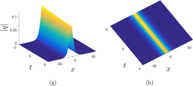
Next, corresponding to equations (36 ), (47 ) and (52 ) we shall obtain multi-soliton solutions of the nonlocal Hirota equations. When N = 1, the soliton solutions for the three types of nonlocal Hirota equations are shown in figure 1, respectively. When N = 2, we plot the graphs of the two-soliton solutions for reverse-time nonlocal Hirota equation as shown in figure 2 by selecting appropriate parameters. Due to the different symmetry conditions between the reverse-time nonlocal Hirota equation and the other two nonlocal Hirota equations, we can obtain the different graphs. It is worth noting that when either λ = −λ* or $\hat{\lambda }=-{\hat{\lambda }}^{* }$. In other words, λ and $\hat{\lambda }$ is purely imaginary, the two-soliton solutions of the reverse-spacetime nonlocal Hirota equation in figure 1 degenerate into the single-soliton solution in figure 3.
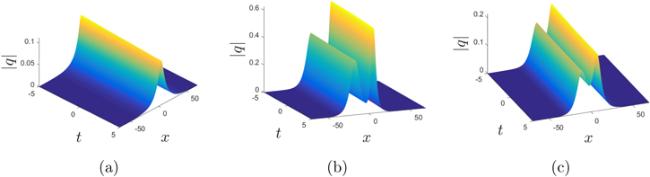
Figure 1. (a) The single-soliton solution via (36) with a = i, b = 0.5i, λ = 0.01 − 0.05i, α1 = 0.1 + 0.1i, β1 = 0.5 + 0.1i. (b) The two-soliton solutions via (47) with a = 0.5, b = 0.1i, λ = 0.2 + 0.1i, $\hat{\lambda }=0.3+0.2{\rm{i}}$, α1 = 0.1 + 0.5i, β1 = 0.1, ${\hat{\alpha }}_{1}=1-0.4{\rm{i}}$, ${\hat{\beta }}_{1}=0.1$. (c) The two-soliton solutions via (52) with a = 0.4i, b = 0.3, λ = 0.06 + 0.1i, $\hat{\lambda }=0.1+0.1{\rm{i}}$, α1 = 0.3 + 0.4i, β1 = 0.25 + 0.2i, ${\hat{\alpha }}_{1}=0.45+0.4{\rm{i}}$, ${\hat{\beta }}_{1}\,=0.4-0.3{\rm{i}}$. |
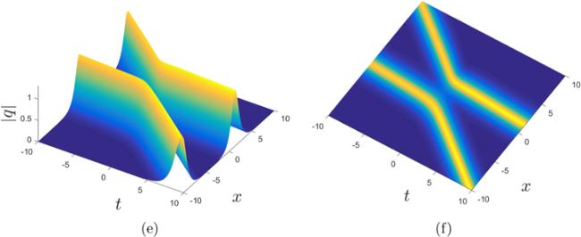
Figure 2. (e) The two-soliton solutions of reverse-time nonlocal Hirota equation via with a = −0.7i, b = 0.4i, λ1 = 0.2 − 0.05i, λ2 = 0.3 +0.1i, α1 = 0.15 + 0.1i, β1 = 0.35 + 0.1i, α2 = 0.4 + 0.08i, β2 = 0.6 − 0.1i. |
Figure 3. Degenerated single-soliton solution of reverse-spacetime nonlocal Hirota equation, where the parameters are chosen as a = 0.4i, b = 0.3, λ = 0.06 + 0.1i, $\hat{\lambda }=0.1{\rm{i}}$, α1 = 0.3 + 0.4i, β1 = 0.25 + 0.2i, ${\hat{\alpha }}_{1}=0.45+0.4{\rm{i}}$, ${\hat{\beta }}_{1}=0.4-0.3{\rm{i}}$. |
4. Conclusion
The aim of the current investigation is to derive multi-soliton solutions of the nonlocal Hirota equations by utilizing the RH approach. To this end, starting firstly from the equivalence spectral problem of the coupled Hirota equations, which effectively acquire the relevant analytical properties, then we construct the RH problem of the nonlocal Hirota equations. Secondly, considering different symmetry relationships, the three types of nonlocal Hirota equations are discussed. After solving the RH problem without reflection, we finally obtain the multi-soliton solutions of the nonlocal Hirota equations, Particularly, the single- and two-soliton solutions are displayed.