


1. Introduction
Soft-collinear factorization is crucial in connecting perturbative QCD calculations with experimental data of high energy hadron processes. Such factorization is proved in many typical processes in the frame of perturbative QCD, (see, for example, [1–8]). Compared to these results, the factorization in soft-collinear effective theory (SCET) [9–12] provides us with a new perspective to understand the QCD factorization, which seems more intuitive. Collinear, soft and ultrasoft particles are described by effective modes in SCET. Especially, the hard collisions between collinear particles are described by various effective operators in SCET. In the original SCET Lagrangian, ultrasoft gluons decouple from collinear fields after a unitary transformation and collinear-soft couplings are absorbed into soft Wilson lines. Thus the soft-collinear factorization holds at the Lagrangian level in the original SCET.
Despite great advantages, the original SCET did not deal with Glauber gluons properly. Glauber gluons, which take space-like momenta, are responsible for elastic scattering processes between different jets. Results in [13] displayed how Glauber gluons break the QCD factorization in processes involving two initial hadrons like the Drell–Yan process. For Drell-Yan process, leading pinch singularities in the Glauber region cancel out according to the unitarity [2–4]. One may then deform the integral path of loop momenta to avoid the Glauber region. After the deformation, couplings between Glauber gluons and collinear particles eikonalize. That is, Glauber gluons behave like soft or collinear gluons after the deformation. In summary, the soft-collinear factorization of the Drell–Yan process is not violated by Glauber gluons [2–4]. However, the factorization can be violated by Glauber gluons for processes that are not inclusive enough (see, for example, [14–18]). In these processes, cancellation of leading pinch singularities in the Glauber region is hindered by Glauber couplings of the detected final particles
Although leading pinch singular singularities in the Glauber region may cancel out, the Glauber gluon effects are visible in processes in which the factorization works. Since the contour deformation to avoid the Glauber region relies on explicit processes, whether the collinear and soft Wilson lines appearing in parton (distribution and fragmentation) functions and soft factors are past-pointing or future-pointing is process dependent [19]. In other words, Glauber gluons affect the directions of various Wilson lines in the factorization. Such effects are more obvious in transverse momentum-dependent objects like the Sivers function [20–22], although they are not concerned here.
Glauber gluons in SCET are more subtle. In [23–27], Glauber gluon fields are added into the SCET Lagrangian to describe jets in dense QCD matter. The effective theory is termed SCETG. Glauber gluons in SCETG behave like a QCD background and do not cause scattering between different jets directly. This is different from the situation one confronts in usual soft-collinear factorization. In [28–30], Glauber gluons are integrated out and effective operators that describe elastic scattering effects between collinear particles are introduced into the effective action of SCET. These operators are nonlocal, in which the decoupling of ultrasoft gluons from collinear fields is no longer manifest. Matching the coefficients of these operators relies on a suitable subtraction scheme [28, 31] to avoid double counting in loop integrals and a systematic scheme [32, 33] to regularize the rapidity divergences. These effective operators may violate the factorization theorem in SCET as they cause coherence between different jets. In [30], the authors discuss the properties of these operators.
In [30], ladder diagrams like those shown in figure 1 were discussed. Explicitly, the ladder diagrams of spectator-spectator Glauber exchanges like those shown in figure 2 cancel out for processes inclusive enough as discussed in [30]. In addition, the ladder-like spectator-active and active–active Glauber exchanges can be absorbed into collinear and Wilson lines according to results in [30].
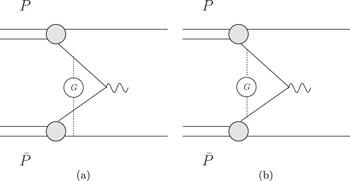
Figure 1. Examples of ladder diagrams with Glauber gluons exchanged (a) between active particles and spectators; (b) between active particles. |
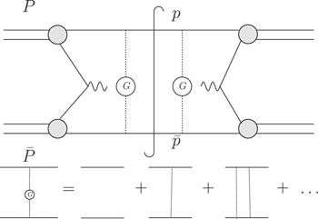
Figure 2. Elastic scattering diagrams between spectators, where the dot lines represent Glauber gluons. |
These discussions are necessary for proofs of the factorization theorem in SCET. However, they are not enough as these discussions are restricted to ladder-like diagrams. More discussions on these topics are necessary. This is the primary motivation of our paper.
Glauber gluons should be viewed as modes different from collinear and soft gluons no matter whether they are integrated out or not. The question is how to distinguish them from collinear and soft gluons in loop integrals. In other words, how to avoid the double counting in loop integrals? Let us start from the coupling between a gluon q and a plus-collinear particle k. If q is soft or ultrasoft or minus-collinear, then the coupling between q and k eikonalize at a leading power of λ. Hence we can define the non-eikonalized part of the coupling as Glaube coupling of k even if q locates in the non-Glauber region without affecting the leading power results. On the other hand, the eikonalized part of the coupling can be absorbed into soft or ultrasoft or collinear Wilson lines even if q locates in the Glauber region. Thus we always define the non-eikonalized part as Glaube coupling of k and absorb the eikonalized part into soft or ultrasoft or collinear Wilson lines. For a Glauber gluon q exchanged between plus-collinear and minus-collinear particles, one has
$\begin{eqnarray}\displaystyle \frac{-{\rm{i}}}{{l}^{2}+{\rm{i}}\varepsilon }\simeq \displaystyle \frac{-{\rm{i}}}{{\left({l}_{\perp }\right)}^{2}+{\rm{i}}\varepsilon }.\end{eqnarray}$
One can also neglect l+(l−) in couplings between l and plus-collinear (minus-collinear) particles. These approximations are helpful to describe the Glauber couplings in loop integrals. Let us consider the coupling between a gluon q and a plus-collinear particle k further. If q is soft or minus-collinear, then the coupling between q and k eikonalize. The eikonalized part of the coupling can be absorbed into collinear or soft Wilson lines and does not affect the factorization even if q locates in the Glauber region. The non-eikonalized part should be power suppressed in the minus-collinear or soft (ultrasoft) region of q. Hence the rapidity divergences in this definition can be controlled through the regulator presented in [30, 32, 33], which reads $\begin{eqnarray}{\omega }^{2}| 2{q}^{z}{| }^{-\eta }{\nu }^{\eta }\propto | {q}^{+}-{q}^{-}{| }^{-\eta }.\end{eqnarray}$
We find it convenient to introduce Glauber gluon fields into the SCET action before integrating them out. This is helpful to determine the power counting for couplings involving Glauber gluons. Especially, it helps us to see the origins of leading power effective operators in [30]. We should mention that the power counting for various modes may depend on explicit gauge conditions in perturbative calculations as shown in [28–30]. Compared to the covariant gauge in [28–30], it is more convenient to work in the Feynman gauge for issues considered here. There are superleading powers in practical diagrams in the Feynman gauge. However, such superleading powers cancel out in physical observable according to the Ward identity [6, 7]. This is confirmed by the power counting result presented in this paper. Thus superleading powers in the Feynman gauge do not disturb us.
The subtraction of eikonalized couplings from the definition of Glauber gluon modes is important in the treatment of elastic scattering processes. The eikonalized part of couplings involving collinear particles should be viewed as soft and collinear and ultrasoft interactions of these collinear particles even if there are gluons with Glauber momenta. Especially, the Glauber couplings of active particles eikonalize and these couplings should be absorbed into the definition of collinear or soft gluons. Besides, the subtraction does not affect spectator-spectator type Glauber gluons in the dimensional regularization scheme after the approximation (1 ) as dimensionless integrals vanish in the scheme.
The paper is organized as follows. In section 2 , we add Glauber gluons into the SCET action. The power counting for couplings involving Glauber gluons is also presented in this section. In section 3 , we discuss how to understand the cancellation of ladder-like Glauber exchanges between spectators presented in [30]. These discussions can be viewed as operator level interpretation of such cancellation. The cancellation of final state interactions for processes inclusive enough is also proved in this section, which is crucial in our general discussions. In section 4 , we consider the Glauber couplings of active particles. We prove the eikonalization of these couplings and explain why these couplings are equivalent to zero bins of soft and collinear couplings of active particles. The absorption of spectator-active Glauber exchanges (including non-ladder-like cases) into collinear Wilson lines and active–soft and active–active Glauber exchanges (including non-ladder-like cases) into collinear Wilson lines is the direct result of discussions in this section. In section 5 , we prove the cross section level cancellation of spectator-spectator Glauber exchanges for processes inclusive enough. We exclude the influence of spectator-active coherence by proving that the coherence should occur before spectator-spectator Glauber exchanges. Hence the summation over final spectators without affecting spectator-active coherence is enough for the cancellation of these Glauber exchanges. After the cancelation, Glauber modes can be absorbed into collinear and soft Wilson lines which are graph independent. In section 6 , we explain how our operator skills are related to the graphic cancellation of spectator–spectator Glauber exchanges in [2–4]. Our conclusions and some discussions are presented in section 7 . In appendix A , we discuss the evolution operator of the effective theory. In appendix B , we discuss how to define spectators and collinear particles. The reparameterization invariance of the effective theory is discussed in appendix C .
2. Glauber gluons in SCET
In this section, we introduce Glauber gluon fields into the SCET action and study Glauber interactions. These discussions are helpful for studies of Glauber effects in hadronic processes at leading power. Glauber gluons take space-like momenta and cause elastic scattering between collinear particles. For example, we consider a gluon with momentum scales as
$\begin{eqnarray}({p}^{+},{p}^{-},{p}_{\perp })\sim Q({\lambda }^{2},{\lambda }^{2},\lambda ),\end{eqnarray}$
where Q represents a hard energy scale and λ ≪ 1. The gluon is space-like as p2 ∼ − Q2λ2 < 0. Exchanging of such gluons causes elastic scattering between particles collinear to the plus and minus directions. We discuss the power counting for couplings between Glauber gluons and other particles in this section. Results in this section are compatible with those in [30] and make our following discussions more clear. $\begin{eqnarray}\int {{\rm{d}}}^{4}x{{\rm{e}}}^{{\rm{i}}k\cdot x}T\lt {A}_{{nG}}^{\mu }(x){A}_{{nG}}^{\nu }(0)\gt =\,\displaystyle \frac{-{\rm{i}}}{{k}^{2}}\left({g}^{\mu \nu }-(1-\xi )\displaystyle \frac{{k}^{\mu }{k}^{\nu }}{{k}^{2}}\right),\end{eqnarray}$
where ξ is the gauge parameter. The power counting for the field An reads $(n\cdot {A}_{n,p},\bar{n}\cdot {A}_{n,p},{A}_{n,{pn}\perp })\sim ({\lambda }^{2},1,\lambda )$. It is required that 1 − ξ is not too small to get this result. While working in the Feynman gauge, there are superleading power terms involving n · An,p in SCET Lagrangian. This does not disturb us as n · An,p and $\bar{n}\cdot {A}_{n,p}$ appear in pairs in practical diagrams. In fact, if there is a collinear gluon polarized as n · An,p, then its other end should polarize as $\bar{n}\cdot {A}_{n,p}$ in the Feynman gauge according to the gμν tensor in its propagator. The power counting for such a pair reads λ2 according to table 1, which is equivalent to that of the covariant gauge in [9, 10].
Table 1. Relevant modes in the propagation of particles collinear to ${n}^{\mu }=\tfrac{1}{\sqrt{2}}(1,\vec{n})$ and the power counting for them in the Feynman gauge, where ${\bar{n}}^{\mu }=\tfrac{1}{\sqrt{2}}(1,-\vec{n})$ and $n\cdot {p}_{n\perp }=\bar{n}\cdot {p}_{n\perp }=0$. |
| Modes | Fields | Momenta scales $(n\cdot p,\bar{n}\cdot p,{p}_{n\perp })$ | Infrared power counting |
|---|---|---|---|
| Collinear quarks | ξn | Q(λ2, 1, λ) | λ |
| Collinear gluons | ${A}_{n}^{\mu }$ | Q(λ2, 1, λ) | λ |
| Soft quarks | ψs | Q(λ, λ, λ) | λ3/2 |
| Soft gluons | ${A}_{s}^{\mu }$ | Q(λ, λ, λ) | λ |
| Ultrasoft quarks | ψus | Q(λ2, λ2, λ2) | λ3 |
| Ultrasoft gluons | ${A}_{{us}}^{\mu }$ | Q(λ2, λ2, λ2) | λ2 |
| Glauber gluons | ${A}_{{nG}}^{\mu }$ | Q(λ2, λb, λ)( b = 1,2) | ${\lambda }^{1+\tfrac{b}{2}}$ |
To obtain the power counting for Glauber gluon fields, we consider the Glauber propagators in the Feynman gauge,
$\begin{eqnarray}\int {{\rm{d}}}^{4}x{{\rm{e}}}^{{\rm{i}}k\cdot x}T\lt {A}_{{nG}}^{\mu }(x){A}_{{nG}}^{\nu }(0)\gt =\,\displaystyle \frac{-{\rm{i}}{g}^{\mu \nu }}{{k}^{2}}.\end{eqnarray}$
The Glauber momentum scale as $(n\cdot k,\bar{n}\cdot k,{k}_{n\perp })\sim Q({\lambda }^{2},{\lambda }^{b},\lambda )$ and the integral volume scale as ∫d4x ∼ Q−4λ−4−b. Thus the power counting for Glauber gluon fields reads ${A}_{{nG}}^{\mu }\sim {\lambda }^{1+\tfrac{b}{2}}$. For future convenience, we present here the power counting for fermions with momenta scales as $(n\cdot k,\bar{n}\cdot k,{k}_{n\perp })\sim Q({\lambda }^{2},{\lambda }^{b},\lambda )$, which reads ${\lambda }^{\tfrac{3+b}{2}}$.2.1. Power counting for couplings between Glauber gluons and other particles
In this section, we consider Glauber interactions. We first consider couplings between Glauber gluons and ultrasoft gluons. According to table 1, the power counting for ultrasoft particles and Glauber gluons reads λ3, λ2 and ${\lambda }^{1+\tfrac{b}{2}}$. The integral volumes of these couplings scale as ∫d4x ∼ Q−4λ−4−b. In these couplings, there are at least two Glauber gluons and one ultrasoft gluon. The power counting for the combination of these fields reads λ4+b. There is an additional gluon field or momentum operator in these couplings according to Lorentz covariance. The power counting for the additional gluon field reads ${\lambda }^{1+\tfrac{b}{2}}$ or λ2. That of the momentum operator reads λ or λ2. Thus the infrared power counting for these couplings reads λr, where
$\begin{eqnarray}r\geqslant 1+4+b+(-4-b)=1.\end{eqnarray}$
That is to say, the infrared power counting for these couplings reads λ or higher. For the couplings between Glauber gluons and ultrasoft fermions, the situation is similar. The integral volumes scale as ∫d4x ∼ Q−4λ−4−b. In these couplings, there are at least one ultrasoft fermion and one Glauber gluon and one fermion with momentum scales as $(n\cdot k,\bar{n}\cdot k,{k}_{n\perp })\sim Q({\lambda }^{2},{\lambda }^{b},\lambda )$. The power counting for these fields reads λ3, ${\lambda }^{1+\tfrac{b}{2}}$ and ${\lambda }^{\tfrac{3+b}{2}}$ respectively. Momenta of these fields are quite small and there are no energy scales that may produce the minus power of λ. Thus the infrared power counting for these couplings reads ${\lambda }^{\tfrac{3}{2}}$ or higher.For the couplings between Glauber gluons without other type particles, the integral volume scales as ∫d4x ∼Q−4λ−4−b. There are at least three Glauber gluons and the power counting for the combination reads ${\lambda }^{3+\tfrac{3b}{2}}$. There is an additional gluon field (${\lambda }^{1+\tfrac{b}{2}}$) or momentum operator (λ or λ2) in these couplings. Thus the power counting for these couplings reads ${\lambda }^{\tfrac{b}{2}}$ or higher.
For the couplings between Glauber gluon fields AnG and ${A}_{\bar{n}G}$, which involve soft gluons, the integral volume scales as ∫d4x ∼ Q−4λ−4. There are at least two Glauber gluons (${\lambda }^{1+\tfrac{b}{2}}$) and one soft gluon (λ) in these couplings. There is an additional gluon (${\lambda }^{1+\tfrac{b}{2}}$ or λ) field or momentum operator (λ or λ2) in these couplings. Thus the power counting for these couplings reads λbor higher.
For the couplings between Glauber gluon fields AnG and soft gluons without Glauber gluon fields ${A}_{\bar{n}G}$, the integral volume scales as ∫d4x ∼ Q−4λ−4. In these couplings, there are at least two soft gluons and one Glauber gluon. The power counting for the combination reads ${\lambda }^{3+\tfrac{b}{2}}$. There is an additional gluon field (${\lambda }^{1+\tfrac{b}{2}}$ or λ) or momentum operator (λ or λ2) in these couplings according to Lorentz invariance. Thus the infrared power counting for these couplings reads ${\lambda }^{\tfrac{b}{2}}$ or higher.
For the couplings between Glauber gluons and soft fermions, the integral volume scales as ∫d4x ∼ Q−4λ−4. In these couplings, there are at least two soft fermions and one Glauber gluon. The power counting for the combination reads ${\lambda }^{4+\tfrac{b}{2}}$. Momenta of these fields are quite small and there are no energy scales that may produce the minus power of λ. Thus the infrared power counting for these couplings reads ${\lambda }^{\tfrac{b}{2}}$ or higher.
For the couplings between Glauber gluon fields AnG and n-collinear fermions, the integral volume scales as ∫d4x ∼Q−4λ−4. In these couplings, there are at least two collinear fermions and one Glauber gluon. The power counting for the combination reads ${\lambda }^{3+\tfrac{b}{2}}$. Thus the power counting for these couplings reads ${\lambda }^{\tfrac{b}{2}-1}$ or higher.
For the couplings between Glauber gluon fields AnG and n-collinear gluons, the integral volume scales as ∫d4x ∼Q−4λ−4. In these couplings, there are at least two collinear gluons and one Glauber gluon. The infrared power counting for the combination reads ${\lambda }^{3+\tfrac{b}{2}}$. There is an additional gluon field (${\lambda }^{1+\tfrac{b}{2}}$ or λ) or momentum operator (λ0, λ or λ2) in these couplings. Thus the power counting for these couplings reads ${\lambda }^{\tfrac{b}{2}-1}$ or higher.
For the couplings between Glauber gluon fields AnG and $\bar{n}$-collinear fermions, the integral volume scales as ∫d4x ∼Q−4λ−2−b. In these couplings, there is at least one collinear fermion, one Glauber gluon and one fermion with momentum scales as $(n\cdot k,\bar{n}\cdot k,{k}_{n\perp })\sim Q(1,{\lambda }^{b},\lambda )$. The power counting for the combination reads ${\lambda }^{3+\tfrac{b}{2}}$. Thus the power counting for these couplings reads ${\lambda }^{1-\tfrac{b}{2}}$ or higher.
For the couplings between Glauber gluon fields AnG and $\bar{n}$-collinear gluons, the integral volume scales as ∫d4x ∼Q−4λ−2−b. In these couplings, there is at least one collinear gluon, one Glauber gluon and one gluon with momentum scales as $(n\cdot k,\bar{n}\cdot k,{k}_{n\perp })\sim Q(1,{\lambda }^{b},\lambda )$. The power counting for the combination of these fields reads ${\lambda }^{3+\tfrac{b}{2}}$ or higher. There is an additional gluon field or momentum operator in these couplings. The power counting for these objects reads λ0 or higher. Thus the power counting for these couplings reads ${\lambda }^{1-\tfrac{b}{2}}$ or higher.
Our results in this section are presented in table 2.
Table 2. The infrared power counting for couplings involving Glauber gluons, where ${\bar{n}}^{\mu }=\tfrac{1}{\sqrt{2}}(1,-\vec{n})$. |
| Couplings | Fields | Power counting |
|---|---|---|
| Glauber gluons and ultrsoft gluons | (AnG,Aus) | λ or higher |
| Glauber gluons and ultrsoft fermions | (AnG,Aus) | ${\lambda }^{\tfrac{3}{2}}$ or higher |
| Glauber gluons | (AnG) | ${\lambda }^{\tfrac{b}{2}}$ or higher |
| Glauber gluons and soft gluons | (AnG,${A}_{\bar{n}G}$,As) | λ or higher |
| Glauber gluons and soft gluons | (AnG,As) | ${\lambda }^{\tfrac{b}{2}}$ or higher |
| Glauber gluons and soft fermions | (AnG,ψs) | ${\lambda }^{\tfrac{b}{2}}$ or higher |
| Glauber gluons and collinear fermions | (AnG,ξn) | ${\lambda }^{\tfrac{b}{2}-1}$ or higher |
| Glauber gluons and collinear gluons | (AnG,An) | ${\lambda }^{\tfrac{b}{2}-1}$ or higher |
| Glauber gluons and collinear fermions | (AnG,${\xi }_{\bar{n}}$) | ${\lambda }^{1-\tfrac{b}{2}}$ or higher |
| Glauber gluons and collinear gluons | (AnG,${A}_{\bar{n}}$) | ${\lambda }^{1-\tfrac{b}{2}}$ or higher |
2.2. Leading power action including Glauber gluons
We consider the leading power SCET action with Glauber gluon fields in this section. There are two kinds of SCET Lagrangian in literature, SCETI and SCETII, which are suitable for studies on different objects. We do not distinguish them here. For simplicity, we neglect the couplings involving ultrasoft particles and the couplings between Glauber gluons without soft gluons at first.
We start from a Glauber gluon AnG which couples to n-collinear particles. The power counting for such coupling reads ${\lambda }^{\tfrac{b}{2}-1}$ according to the results in table 2. The other end of the Glauber gluon may couple to ultrasoft particles, Glauber gluons, soft particles or particles collinear to other directions. If the Glauber gluon couple to particles collinear to other directions at that end, then the power counting for that coupling reads ${\lambda }^{1-\tfrac{b}{2}}$. The final power counting for couplings at two ends of the Glauber gluon reads λ0.4(There may be additional powers of λ in practical diagrams even if these diagrams involve only leading order couplings as shown in [30]. This does not disturb us here as we are only concerned with the power counting for effective iterations in this paper.)
If the other end of the Glauber gluon involves soft particles, then the power counting for that coupling reads ${\lambda }^{\tfrac{b}{2}}$ or λ. For the former case, the final power counting for couplings at two ends of the Glauber gluon reads λb−1 ≥ λ0. For the latter case, in which b = 1, the other end of AnG involves a Glauber gluon of the type ${A}_{\bar{n}G}$. If the other end of the ${A}_{\bar{n}G}$ couple to particles collinear to ${\bar{n}}^{\mu }$, then the final power counting for these couplings reads ${\lambda }^{-\tfrac{1}{2}+1-\tfrac{1}{2}}={\lambda }^{0}$. If the other end of ${A}_{\bar{n}G}$ couples to soft particles, then we can repeat the procedure and get the same result. In conclusion, the final power counting for these couplings reads λ0 if there are couplings between Glauber gluons and soft particles.
If a Glauber gluon is exchanged between soft particles, then the power counting for the combination of couplings at the two ends of the diagram reads, λb ≥ λ1. We notice that the minus powers of λ can only be produced by couplings between glauber gluons and collinear particles. Thus the combination of couplings involving Glauber gluons is power suppressed except for those couplings between Glauber gluons and collinear particles are involved.
We then consider couplings involving ultrasoft particles and couplings between Glauber gluons without soft gluons. The power counting for the couplings between Glauber gluons and ultrasoft particles reads λ1 or λ3/2. The power counting for couplings between Glauber gluons without soft gluons reads ${\lambda }^{\tfrac{b}{2}}$.5(One should not be confused with the possible fractional power in this coupling. There are other powers of λ in diagrams involving this coupling. For example, one considers the coupling between three Glauber gluons of the type AnG. Two of them connect to a fermion collinear to nμ and one of them collinear to ${\bar{n}}^{\mu }$. At leading power, two of them are of the type $\bar{n}\cdot {A}_{G}$ and one of them is of the type n · AG in the coupling between these three Glauber gluons. According to Lorentz covariance, there is a momentum term of the type n · k ∼ λ2 instead of the type k⊥ ∼ λ, which is produced by the coupling between the three Glauber gluons. Thus the power counting for the combination of these couplings reads ${\lambda }^{\tfrac{b}{2}-1}{\lambda }^{\tfrac{b}{2}-1}{\lambda }^{1-\tfrac{b}{2}}{\lambda }^{\tfrac{b}{2}}{\lambda }^{2-1}={\lambda }^{b}$.) According to the above discussions, the combination of other couplings involving Glauber gluons does not produce minus powers of λ. Thus couplings involving ultrasoft particles and couplings between Glauber gluons without soft gluons are power suppressed.
In Summary, (1) Glauber gluons are exchanged between collinear particles and soft particles or between collinear particles at leading power; (2) there may be intermediate couplings between Glauber gluons and soft particles in these exchanges at leading power; (3) couplings between Glauber gluons and ultrasoft particles are power suppressed; (4) couplings between Glauber gluons without soft gluons are power suppressed. This is compatible with the results in [30].
The leading power effective action can then be written as6(The perpendicular components ${A}_{{nG}\perp }^{\mu }$ decouple from other fields at the leading power of λ. We simply disregard them here.),7(We should mention that there is overlap between ${A}_{{nG}}^{\mu }$ and ${A}_{\bar{n}G}^{\mu }$, which should be subtracted from the effective action. The subtraction is not displayed here for simplicity.)
$\begin{eqnarray}{I}_{{\rm{eff}}}=\sum _{n}{I}_{n}^{G}+{I}_{s}^{G}+{I}_{{us}}+\sum _{n}{I}_{{nG}}\end{eqnarray}$
$\begin{eqnarray}\begin{array}{rcl}{I}_{n}^{G} & = & \displaystyle \int {{\rm{d}}}^{4}x{\bar{\xi }}_{n}\{{\rm{i}}n\cdot D+{gn}\cdot ({A}_{n}+{A}_{{nG}})\\ & & +({{/}\!\!\!\!{{ \mathcal P }}}_{\perp }+g{{/}\!\!\!\!{A}}_{n}^{\perp }){W}_{n}\displaystyle \frac{1}{\bar{{ \mathcal P }}}{W}_{n}^{\dagger }({{/}\!\!\!\!{{ \mathcal P }}}_{\perp }+g{{/}\!\!\!\!{A}}_{n}^{\perp })\}{/}\!\!\!\!{\bar{n}}{\xi }_{n}\\ & & +\displaystyle \int {{\rm{d}}}^{4}x\displaystyle \frac{1}{2{g}^{2}}{\rm{tr}}\{[{\rm{i}}{{ \mathcal D }}_{{nG}}^{\mu }+{{gA}}_{n}^{\mu },{\rm{i}}{{ \mathcal D }}_{{nG}}^{\nu }+{{gA}}_{n}^{\nu }]\}{}^{2}\\ & & +\displaystyle \int {{\rm{d}}}^{4}x2{\rm{tr}}\{{\bar{c}}_{n}[{\rm{i}}{{ \mathcal D }}_{n\mu },[{\rm{i}}{{ \mathcal D }}_{{nG}}^{\mu }+{{gA}}_{n}^{\mu },{c}_{n}]]\}\\ & & +\displaystyle \int {{\rm{d}}}^{4}{x}{\rm{tr}}\{[{\rm{i}}{{ \mathcal D }}_{n\mu },{A}_{n}^{\mu }+{gn}\cdot {A}_{{nG}}{\bar{n}}^{\mu }]\\ & & \times [{\rm{i}}{{ \mathcal D }}_{n\nu },{A}_{n\nu }+{gn}\cdot {A}_{{nG}}{\bar{n}}^{\nu }]\}\end{array}\end{eqnarray}$
$\begin{eqnarray}\begin{array}{rcl}{I}_{s}^{G} & = & \displaystyle \int {{\rm{d}}}^{4}x{\bar{\psi }}_{s}({/}\!\!\!\!{{ \mathcal P }}+g{{/}\!\!\!\!{A}}_{s}+g{/}\!\!\!\!{\bar{n}}\sum _{n}\bar{n}\cdot {A}_{{nG}}){\psi }_{s}\\ & & -\displaystyle \frac{1}{2}\displaystyle \int {{\rm{d}}}^{4}{x}{\rm{tr}}\{{G}_{s}^{\mu \nu }{G}_{\mu \nu }^{s}\}\\ & & +\displaystyle \int {{\rm{d}}}^{4}x2{\rm{tr}}\{{\bar{c}}_{s}[{{ \mathcal P }}_{\mu },[{{ \mathcal P }}^{\mu }+{{gA}}_{s}^{\mu }\\ & & +g\sum _{n}\bar{n}\cdot {A}_{{nG}}{n}^{\mu },{c}_{s}]]\}\\ & & +\displaystyle \int {{\rm{d}}}^{4}{x}{\rm{tr}}\{[{{ \mathcal P }}_{\mu },{A}_{s}^{\mu }+g\sum _{n}\bar{n}\cdot {A}_{{nG}}{n}^{\mu }]\\ & & \times [{{ \mathcal P }}_{\nu },{A}_{s\nu }+g\sum _{n}\bar{n}\cdot {A}_{{nG}}{n}^{\nu }]\}\end{array}\end{eqnarray}$
$\begin{eqnarray}\begin{array}{rcl}{I}_{{us}} & = & \displaystyle \int {{\rm{d}}}^{4}x{\bar{\psi }}_{{us}}{/}\!\!\!\!{D}{\psi }_{{us}}-\displaystyle \int {{\rm{d}}}^{4}x\displaystyle \frac{1}{2}\{{G}_{\mu \nu }{G}^{\mu \nu }\}\\ & & +\displaystyle \int {{\rm{d}}}^{4}x2{\rm{tr}}\{{\bar{c}}_{{us}}[i{\partial }_{\mu },[{\rm{i}}{D}^{\mu },{c}_{{us}}]]\}\\ & & +\displaystyle \int {{\rm{d}}}^{4}{x}{\rm{tr}}[{\left(\partial \cdot {A}_{{us}}\right)}^{2}]\end{array}\end{eqnarray}$
$\begin{eqnarray}\begin{array}{rcl}{I}_{{nG}} & = & \displaystyle \int {{\rm{d}}}^{4}{x}{\rm{tr}}[({{ \mathcal P }}^{\mu }\bar{n}\cdot {A}_{{nG}})(({{ \mathcal P }}_{\mu }n\cdot {A}_{{nG}})]\\ & & -\displaystyle \frac{1}{4}\displaystyle \int {{\rm{d}}}^{4}{x}{\rm{tr}}[(\bar{n}\cdot { \mathcal P }n\cdot {A}_{{nG}})(\bar{n}\cdot { \mathcal P }n\cdot {A}_{{nG}})],\end{array}\end{eqnarray}$
where (ξn, An, cn) are collinear fields and (ψs, As) are soft fields and (ψus, Aus) are ultrasoft fields and
$\begin{eqnarray}{W}_{n}(x)=P\exp ({\rm{i}}g{\int }_{-\infty }^{0}{\rm{d}}s\bar{n}\cdot {A}_{n}(x+s\bar{n}))\end{eqnarray}$
$\begin{eqnarray}{D}^{\mu }={\partial }^{\mu }-{\rm{i}}{{gA}}_{{us}}^{\mu }\end{eqnarray}$
$\begin{eqnarray}\begin{array}{l}{{ \mathcal P }}^{\mu }({\phi }_{{q}_{1}}^{\dagger }\cdot \cdot \cdot {\phi }_{{q}_{m}}^{\dagger }{\phi }_{{p}_{1}}\cdot \cdot \cdot {\phi }_{{p}_{n}})\\ \quad =({p}_{1}^{\mu }\,+\cdots +\,{p}_{n}^{\mu }-{q}_{1}^{\mu }\cdots -{q}_{m}^{\mu })({\phi }_{{q}_{1}}^{\dagger }\cdot \cdot \cdot {\phi }_{{q}_{m}}^{\dagger }{\phi }_{{p}_{1}}\cdot \cdot \cdot {\phi }_{{p}_{n}})\end{array}\end{eqnarray}$
$\begin{eqnarray}{\rm{i}}{{ \mathcal D }}_{n}^{\mu }={n}^{\mu }\bar{n}\cdot { \mathcal P }+{{ \mathcal P }}_{\perp }^{\mu }+{\bar{n}}^{\mu }{\rm{i}}n\cdot D\end{eqnarray}$
$\begin{eqnarray}\begin{array}{rcl}{\rm{i}}{G}_{s}^{\mu \nu } & = & \displaystyle \frac{1}{g}[{{ \mathcal P }}^{\mu }+{{gA}}_{s}^{\mu }+g\sum _{n}\bar{n}\cdot {A}_{{nG}}{n}^{\mu },{{ \mathcal P }}^{\nu }+{{gA}}_{s}^{\nu }\\ & & +g\sum _{n}\bar{n}\cdot {A}_{{nG}}{n}^{\nu }]\end{array}\end{eqnarray}$
$\begin{eqnarray}\begin{array}{rcl}{G}^{\mu \nu } & = & \displaystyle \frac{{\rm{i}}}{g}[{D}^{\mu },{D}^{\nu }]\\ {{ \mathcal D }}_{{nG}}^{\mu } & = & {{ \mathcal D }}_{n}^{\mu }-{\bar{n}}^{\mu }{\rm{i}}{gn}\cdot ({A}_{{nG}}).\end{array}\end{eqnarray}$
Some power suppressed terms are added into the action to maintain the BRST covariance as discussed in appendix A . We see that diagrams involving AnG(k) rely on n · k through various propagators and vertexes involving AnG(k) are independent of n · k at leading power. This is crucial in our following discussions.
Before the end of this section, we briefly discuss the Glauber gluon states. Although the momenta square of Glauber gluon modes is of order Q2λ2 like those of collinear and soft particles, there are not time derivative terms of Glauber gluon modes in the leading power action (7 ). Hence Glauber gluons should be viewed as constraints not canonical variables in the effective theory. In other words, Glauber gluon fields do not correspond to quantum physical states. On the other hand, one may try to solve the constraint, which is equivalent to integrating out Glauber gluon fields. We show the motion equation of Glauber gluon fields in appendix A . While referring to Glauber gluon states, we always mean the states corresponding to the field configuration of the solution of Glauber gluons. In other words, the relevant quantum states in the soft-collinear factorization are not changed by Glauber gluon fields.
3. Elastic scattering effects in hadron collisions
In this section, we consider the kinematic effects of Glauber gluons and prove the cancellation of final state interactions in inclusive processes. These discussions are independent of the details of Glauber couplings.
The processes considered here can be written as,
$\begin{eqnarray}{H}_{1}(P)+{H}_{2}(\bar{P})\to {l}^{+}{l}^{-}(q)+X\end{eqnarray}$
or $\begin{eqnarray}{H}_{1}(P)+{H}_{2}(\bar{P})\to {J}_{3}({P}_{3})+{J}_{4}({P}_{4})+X\end{eqnarray}$
with P3 + P4 = q, where H1 and H2 represent the initial hadrons with momenta P and $\bar{P}$ and l+l−(q) represents a lepton pair with momentum q and J3 and J4 represent the detected final jets with momenta P3 and P4 and X represents any other states. We work in the center of mass frame of initial hadrons. At leading power of ${{\rm{\Lambda }}}_{{QCD}}/{\left({q}^{2}\right)}^{1/2}$, P and $\bar{P}$ are light-like. Without loss of generality, we assume that Pμ is plus-collinear and ${\bar{P}}^{\mu }$ is minus-collinear.The hard subprocess is described by a hard vertex, which is denoted as J(x). For example, the hard electromagnetic vertex in SCETII takes the form [30],
$\begin{eqnarray}J={\bar{\xi }}_{n}{W}_{n}{S}_{n}^{\dagger }{\rm{\Gamma }}{S}_{\bar{n}}{W}_{\bar{n}}^{\dagger }{\xi }_{\bar{n}},\end{eqnarray}$
where Wn and ${W}_{\bar{n}}$ are collinear Wilson lines and Sn and ${S}_{\bar{n}}$ are soft Wilson lines.We do not consider quantities dependent on q⊥ in this paper. Thus one can integrate out q⊥ in the following discussion.
3.1. Elastic scattering effects without interactions between spectators and active particles
In this section, we start from spectator–spectator interactions without the active-spectator coherence8(Effects of the active-spectator coherence are discussed in sections 5.2 –5.4 .). We show an operator level explanation for the spectator–spectator cancellations discussed in [30]. Our explanation based on the unitarity is quite general and helpful to understand what happens in inclusive processes. Given that the active-spectator coherence is neglected, such cancelation can be easily extended to non-Glauber interactions.
Let us start from the diagrams shown in figure 2. These diagrams can be written as,
$\begin{eqnarray}\begin{array}{l}S(P,\bar{P},p,\bar{p})\equiv \displaystyle \int {{\rm{d}}}^{4}{x}_{1}\displaystyle \int {{\rm{d}}}^{4}{x}_{2}\displaystyle \int {{\rm{d}}}^{4}{x}_{3}\displaystyle \int {{\rm{d}}}^{4}{x}_{4}\\ \quad \times \displaystyle \int {{\rm{d}}}^{4}z{{\rm{e}}}^{{\rm{i}}(P+\bar{P}-p-\bar{p})\cdot z}\\ \quad \times \left\langle P\bar{P}| \bar{T}\{{{ \mathcal O }}^{\dagger }({x}_{1}){\bar{{ \mathcal O }}}^{\dagger }({x}_{2}){J}^{\dagger }(z){U}^{\dagger }(\infty ,-\infty )\}| p\bar{p}\right\rangle \\ \quad \times \left\langle p\bar{p}| T\{{ \mathcal O }({x}_{3})\bar{{ \mathcal O }}({x}_{4})J(0)U(\infty ,-\infty )\}| P\bar{P}\right\rangle ,\end{array}\end{eqnarray}$
where T and $\bar{T}$ represent the time order and anti-time order operators and J(x) represents the hard vertexes that annihilate active particles and O(x)($\bar{O}(x)$) represents the vertex that produces active particles and spectators from H1($\bar{{H}_{2}}$)and U(t1, t2) represents the time evolution operator of the effective theory in the interaction picture.If we neglect the active-spectator coherence, then the effective action can be written as
$\begin{eqnarray}I={I}_{{ac}}({\psi }_{{ac}},{A}_{{ac}}^{\mu })+{I}_{{sp}}({\psi }_{{sp}},{A}_{{sp}}^{\mu }),\end{eqnarray}$
where Iac is the active part of Ieff and Isp is the spectator part of Ieff9(Given that the active-spectator coherence is neglected, such decomposition is feasible. Otherwise, there should be active-spectator coherence terms.). The interactions between spectators and active particles have been dropped in the above decomposition. We have $\begin{eqnarray}U({t}_{1},{t}_{2})={U}_{{ac}}({t}_{1},{t}_{2}){U}_{{sp}}({t}_{1},{t}_{2})={U}_{{sp}}({t}_{1},{t}_{2}){U}_{{ac}}({t}_{1},{t}_{2}),\end{eqnarray}$
where Uac(t1, t2) and Usp(t1, t2) represent the time evolution operators corresponding to Iac and Isp.We now consider the Wick contractions of the fields in (21 ). Fields in Usp do not contract with those in the current J as J is functional of active particle fields. We notice that the energy of spectators flows out of the vertexes ${ \mathcal O }$ and $\bar{{ \mathcal O }}$. Hence the couplings involving spectators all occur after the production of them. Especially, the interactions corresponding to Usp should occur after the vertexes ${ \mathcal O }$($\bar{{ \mathcal O }}$). As a result, we can drop the contractions between ${ \mathcal O }$($\bar{{ \mathcal O }}$) and Usp once the time coordinates of fields in Usp are smaller than those of ${ \mathcal O }$($\bar{{ \mathcal O }}$). We have
$\begin{eqnarray}\begin{array}{l}\left\langle P\bar{P}| \bar{T}\{{{ \mathcal O }}^{\dagger }({x}_{1}){\bar{{ \mathcal O }}}^{\dagger }({x}_{2}){J}^{\dagger }(z){U}^{\dagger }(\infty ,-\infty )\}| p\bar{p}\right\rangle \\ \quad =\left\langle P\bar{P}| \bar{T}\{{{ \mathcal O }}^{\dagger }({x}_{1}){\bar{{ \mathcal O }}}^{\dagger }({x}_{2}){J}^{\dagger }(z){U}_{{ac}}^{\dagger }(\infty ,-\infty )\}\right.\\ \quad \left.{U}_{{sp}}^{\dagger }(\infty ,-\infty )| p\bar{p}\right\rangle ,\end{array}\end{eqnarray}$
$\begin{eqnarray}\begin{array}{l}\left\langle p\bar{p}| T\{{ \mathcal O }({x}_{3})\bar{{ \mathcal O }}({x}_{4})J(0)U(\infty ,-\infty )\}| P\bar{P}\right\rangle \\ \quad =\left\langle p\bar{p}| {U}_{{sp}}(\infty ,-\infty )T\{{ \mathcal O }({x}_{3})\bar{{ \mathcal O }}({x}_{4})J(0){U}_{{ac}}\right.\\ \quad \left.\times (\infty ,-\infty )\}| P\bar{P}\right\rangle .\end{array}\end{eqnarray}$
We then consider the evolution of the final state $\left|p\bar{p}\right\rangle $ under Usp( ∞ , − ∞ ). Elastic scattering processes exchange the transverse momenta and colors and angular momenta between collinear particles. On the other hand, the total momentum and color and angular momentum of these particles are invariant in the elastic processes. Thus all possible pairs $\left|p\bar{p}\right\rangle $ with fixed total momenta and colors and spins form an invariant subspace of Usp if we neglect inelastic scattering between spectators. That is,
$\begin{eqnarray}\begin{array}{l}\sum \int {{\rm{d}}}^{2}{\rm{\Delta }}{p}_{\perp }{U}_{{sp}}^{\dagger }(\infty ,-\infty )\left|p\bar{p}\right\rangle \left\langle p\bar{p}\right|{U}_{{sp}}(\infty ,-\infty )\\ \quad =\sum \int {{\rm{d}}}^{2}{\rm{\Delta }}{p}_{\perp }\left|p\bar{p}\right\rangle \left\langle p\bar{p}\right|{U}_{{sp}}^{\dagger }(\infty ,-\infty ){U}_{{sp}}(\infty ,-\infty )\\ \quad =\sum \int {{\rm{d}}}^{2}{\rm{\Delta }}{p}_{\perp }\left|p\bar{p}\right\rangle \left\langle p\bar{p}\right|,\end{array}\end{eqnarray}$
where the summation is made over all possible color and angular momentum distributions of the pair $p\bar{p}$ with fixed total color and angular momentum. Δp⊥ is defined as $\begin{eqnarray}{\rm{\Delta }}{p}_{\perp }\equiv {p}_{\perp }-{\bar{p}}_{\perp }.\end{eqnarray}$
We then have, $\begin{eqnarray}\begin{array}{l}\sum \int {{\rm{d}}}^{2}{\rm{\Delta }}{p}_{\perp }S(P,\bar{P},p,\bar{p})\\ \quad \equiv \sum \int {{\rm{d}}}^{2}{\rm{\Delta }}{p}_{\perp }\int {{\rm{d}}}^{4}{x}_{1}\int {{\rm{d}}}^{4}{x}_{2}\int {{\rm{d}}}^{4}{x}_{3}\int {{\rm{d}}}^{4}{x}_{4}\\ \quad \times \displaystyle \int {{\rm{d}}}^{4}z{{\rm{e}}}^{{\rm{i}}(P+\bar{P}-p-\bar{p})\cdot z}\\ \quad \times \left\langle P\bar{P}| \bar{T}\{{{ \mathcal O }}^{\dagger }({x}_{1}){\bar{{ \mathcal O }}}^{\dagger }({x}_{2}){J}^{\dagger }(z){U}_{{ac}}^{\dagger }(\infty ,-\infty )\}| p\bar{p}\right\rangle \\ \quad \times \left\langle p\bar{p}| T\{{ \mathcal O }({x}_{3})\bar{{ \mathcal O }}({x}_{4})J(0){U}_{{ac}}(\infty ,-\infty )\}| P\bar{P}\right\rangle .\end{array}\end{eqnarray}$
Thus the elastic scattering effects between spectators cancel out in processes inclusive enough once we neglect the active-spectator coherence. Such cancellation is independent of the details of elastic interactions between spectators.If there are inelastic interactions involving spectators like those shown in figure 3, then the summation over all possible soft and ultrasoft final states is necessary. That is,
$\begin{eqnarray}\begin{array}{l}\sum _{p,\bar{p},\ldots ,}{U}_{{sp}}^{\dagger }(\infty ,-\infty )\left|p\bar{p}\ldots \right\rangle \left\langle p\bar{p}\ldots \right|{U}_{{sp}}(\infty ,-\infty )\\ \quad =\sum _{p,\bar{p},\ldots ,}\left|p\bar{p}\ldots \right\rangle \left\langle p\bar{p}\ldots \right|,\end{array}\end{eqnarray}$
where the summation is made over all possible final particles with fixed total momentum and color and angular momentum. Thus the spectator–spectator interactions cancel out in processes inclusive enough given that the active-spectator coherence haven been dropped as in figure 3.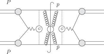
Figure 3. An example of diagrams without the active-spectator coherence. |
3.2. Cancellation of final state interactions
In this section, we take into account the active-spectator coherence and prove the cancellation of final state interactions in the process is inclusive enough. Such general cancellation originates from the unitarity.
For diagrams with the active-spectator coherence, like those shown in figure 4 and their conjugations, the situation is more complicated. Let us consider the quantity,23 ) does not simply work.
$\begin{eqnarray}\begin{array}{l}{ \mathcal H }(P,\bar{P},{q}^{+},{q}^{-})\equiv \sum _{X}\displaystyle \int \displaystyle \frac{{{\rm{d}}}^{2}{q}_{\perp }}{{\left(2\pi \right)}^{2}}\displaystyle \int {{\rm{d}}}^{4}{x}_{1}\displaystyle \int {{\rm{d}}}^{4}{x}_{2}\\ \quad \times \displaystyle \int {{\rm{d}}}^{4}{x}_{3}\displaystyle \int {{\rm{d}}}^{4}{x}_{4}\displaystyle \int {{\rm{d}}}^{4}z{{\rm{e}}}^{{\rm{i}}q\cdot z}\\ \quad \times \left\langle P\bar{P}| \bar{T}\{{{ \mathcal O }}^{\dagger }({x}_{1}){\bar{{ \mathcal O }}}^{\dagger }({x}_{2}){J}^{\dagger }(z){U}^{\dagger }(\infty ,-\infty )\}| H(q)X\right\rangle \\ \quad \times \left\langle H(q)X| T\{{ \mathcal O }({x}_{3})\bar{{ \mathcal O }}({x}_{4})J(0)U(\infty ,-\infty )\}| P\bar{P}\right\rangle ,\end{array}\end{eqnarray}$
where H(q) represents the detected lepton or jet pair with total momenta q and the summation is made over all possible final states. Generally, there is active-spectator coherence in U(t1, t2) and the factorization (
Figure 4. An example of diagrams with the active-spectator coherence. |
Fortunately, the contractions between ${ \mathcal O }$($\bar{{ \mathcal O }}$) and other fields occur only if the time coordinates of fields in ${ \mathcal O }(x)$ are smaller than those of other fields. Otherwise, the contraction does not contribute to ${ \mathcal H }$. We can write ${ \mathcal H }$ as
$\begin{eqnarray}\begin{array}{l}{ \mathcal H }(P,\bar{P},{q}^{+},{q}^{-})\equiv \sum _{X}\displaystyle \int \displaystyle \frac{{{\rm{d}}}^{2}{q}_{\perp }}{{\left(2\pi \right)}^{2}}\displaystyle \int {{\rm{d}}}^{4}{x}_{1}\displaystyle \int {{\rm{d}}}^{4}{x}_{2}\\ \quad \times \displaystyle \int {{\rm{d}}}^{4}{x}_{3}\displaystyle \int {{\rm{d}}}^{4}{x}_{4}\displaystyle \int {{\rm{d}}}^{4}z{{\rm{e}}}^{{\rm{i}}q\cdot z}\\ \quad \times \left\langle P\bar{P}| {{ \mathcal O }}^{\dagger }({x}_{1}){\bar{{ \mathcal O }}}^{\dagger }({x}_{2})\bar{T}\{{J}^{\dagger }(z){U}^{\dagger }(\infty ,-\infty )\}| H(q)X\right\rangle \\ \quad \times \left\langle H(q)X| T\{J(0)U(\infty ,-\infty )\}{ \mathcal O }({x}_{3})\bar{{ \mathcal O }}({x}_{4})| P\bar{P}\right\rangle ,\end{array}\end{eqnarray}$
where the order between operators ${ \mathcal O }$ and $\bar{{ \mathcal O }}$ does not affect the result.We notice that
$\begin{eqnarray}\begin{array}{l}T\{J(x)U(\infty ,-\infty )\}=U(\infty ,{x}^{0})J(x)U({x}^{0},-\infty )\\ \quad =U(\infty ,\max \{{x}^{0},0\})U(\max \{{x}^{0},0\},{x}^{0})J(x)U({x}^{0},-\infty ),\end{array}\end{eqnarray}$
and have $\begin{eqnarray}\begin{array}{l}{ \mathcal H }(P,\bar{P},{q}^{+},{q}^{-})\\ \quad \equiv \sum _{X}\displaystyle \int \displaystyle \frac{{{\rm{d}}}^{2}{q}_{\perp }}{{\left(2\pi \right)}^{2}}\displaystyle \int {{\rm{d}}}^{4}{x}_{1}\displaystyle \int {{\rm{d}}}^{4}{x}_{2}\displaystyle \int {{\rm{d}}}^{4}{x}_{3}\displaystyle \int {{\rm{d}}}^{4}{x}_{4}\displaystyle \int {{\rm{d}}}^{4}z{{\rm{e}}}^{{\rm{i}}q\cdot z}\\ \quad \times \left\langle P\bar{P}\right|{{ \mathcal O }}^{\dagger }({x}_{1}){\bar{{ \mathcal O }}}^{\dagger }({x}_{2})\bar{T}\{{J}^{\dagger }(z){U}^{\dagger }(\max \{{x}^{0},0\},-\infty )\}{U}^{\dagger }\\ \quad \times (\infty ,-\max \{{x}^{0},0\})\left|H(q)X\right\rangle \\ \quad \times \left\langle H(q)X\right|U(\infty ,\max \{{x}^{0},0\})\\ \quad \times T\{J(0)U(\max \{{x}^{0},0\},-\infty )\}{ \mathcal O }({x}_{3})\bar{{ \mathcal O }}({x}_{4})\left|P\bar{P}\right\rangle .\end{array}\end{eqnarray}$
The summation in the above quantity is made over all possible final states. The completeness of the final states X10(X represents all possible other states. Hence H(q)X represents all possible states that contain the detected lepton or jet pair. H(q)X forms the invariant subspace of QCD evolution unless one considers more hard processes after the hard collision(so that the jet pair may vanish). Effects of such hard processes are power suppressed in ${ \mathcal H }(P,\bar{P},{q}^{+},{q}^{-})$ according to the physical picture of pinch singular surfaces [6, 34].) and the unitarity of U(t1, t2) hint that $\begin{eqnarray}\begin{array}{l}\sum _{X}\displaystyle \int \displaystyle \frac{{{\rm{d}}}^{2}{q}_{\perp }}{{\left(2\pi \right)}^{2}}{U}^{\dagger }(\infty ,-\max \{{x}^{0},0\})\left|H(q)X\right\rangle \\ \quad \times \left\langle H(q)X\right|U(\infty ,\max \{{x}^{0},0\})\\ \quad =\sum _{X}\displaystyle \int \displaystyle \frac{{{\rm{d}}}^{2}{q}_{\perp }}{{\left(2\pi \right)}^{2}}\left|H(q)X\right\rangle \left\langle H(q)X\right|\\ \quad \times {U}^{\dagger }(\infty ,-\max \{{x}^{0},0\})U(\infty ,\max \{{x}^{0},0\})\\ \quad =\sum _{X}\displaystyle \int \displaystyle \frac{{{\rm{d}}}^{2}{q}_{\perp }}{{\left(2\pi \right)}^{2}}\left|H(q)X\right\rangle \left\langle H(q)X\right|.\end{array}\end{eqnarray}$
We have, $\begin{eqnarray}\begin{array}{l}{ \mathcal H }(P,\bar{P},{q}^{+},{q}^{-})\\ \quad \equiv \sum _{X}\displaystyle \int \displaystyle \frac{{{\rm{d}}}^{2}{q}_{\perp }}{{\left(2\pi \right)}^{2}}\displaystyle \int {{\rm{d}}}^{4}{x}_{1}\displaystyle \int {{\rm{d}}}^{4}{x}_{2}\displaystyle \int {{\rm{d}}}^{4}{x}_{3}\\ \quad \times \displaystyle \int {{\rm{d}}}^{4}{x}_{4}\displaystyle \int {{\rm{d}}}^{4}z{{\rm{e}}}^{{\rm{i}}q\cdot z}\\ \quad \times \left\langle P\bar{P}| {{ \mathcal O }}^{\dagger }({x}_{1}){\bar{{ \mathcal O }}}^{\dagger }({x}_{2})\bar{T}\{{J}^{\dagger }(z)\right.\\ \quad \left.\times {U}^{\dagger }(\max \{{x}^{0},0\},-\infty )\}| H(q)X\right\rangle \\ \quad \times \left\langle H(q)X| T\{J(0)U(\max \{{x}^{0},0\},-\infty )\}{ \mathcal O }\right.\\ \quad \left.\times ({x}_{3})\bar{{ \mathcal O }}({x}_{4})| P\bar{P}\right\rangle .\end{array}\end{eqnarray}$
Hence final state interactions cancel out in ${ \mathcal H }(P,\bar{P},{q}^{+},{q}^{-})$. This is compatible with the results in [2–4].Especially, the effects of couplings between Glauber gluons and final active particles cancel out in ${ \mathcal H }$ as these couplings occur after the hard collision.
4. Glauber gluons coupling to active particles
In this section, we consider the Glauber couplings of active particles. They are absorbed into collinear and soft Wilson lines for ladder diagram cases [30]. We extend the conclusion to the general situation in this section. Explicitly we see that (1) the active-soft Glauber exchanges can be absorbed into soft Wilson lines in ${ \mathcal H }(P,\bar{P},{q}^{+},{q}^{-})$; (2) the active–active Glauber exchanges can be absorbed into soft Wilson lines in ${ \mathcal H }(P,\bar{P},{q}^{+},{q}^{-})$; (3) the active-spectator Glauber exchanges can be absorbed into collinear Wilson lines in ${ \mathcal H }(P,\bar{P},{q}^{+},{q}^{-})$. We should emphasize that these results are the case even if there is active-spectator coherence.
Glauber gluons look like special collinear or soft gluons. For example, the Glauber gluons ${A}_{{nG}}^{\mu }$ can be viewed as the collinear gluons ${A}_{n,p}^{\mu }$ with $\bar{n}\cdot p=0$ or the soft gluons ${A}_{s,q}^{\mu }$ with n · q = 0. As we always integral over all loop momenta regions in practical diagrams, distinguishing different modes in the loop integrals is quite technical. In perturbative QCD, gluons coupling to active particles are not pinched in the Glauber region [2–4]. As a result, one can deform the integral contour to avoid the Glauber region of these gluons. In SCET, one needs systematic subtraction schemes of which the details are beyond the scope of this paper. We emphasize that whatever the subtraction scheme is, the eikonal approximation is important while dealing with the couplings between collinear and other particles.
The key point is the eikonalization of couplings between Glauber gluons and active particles. As a sequence, Glauber gluons behave like soft or collinear gluons while coupling to active particles. This provides us with the possibility to absorb these Glauber into the definition of soft or collinear gluons. Even if one is not concerned with the definition of different modes, absorption of these Glauber gluons into soft or collinear Wilson lines is the direct result of the eikonlization.
We do not consider the Glauber couplings of final particles as they cancel out in ${ \mathcal H }(P,\bar{P},{q}^{+},{q}^{-})$ (35 ). Without loss of generality, we consider the Glauber couplings of plus-collinear particles in this section. Explicitly, we consider the couplings between some Glauber gluons l1,…,ln and a plus-collinear active particle k in the following sections.
4.1. Eikonal approximation in couplings between collinear particles and soft (ultrasoft) gluons
In this section, we briefly explain the eikonal approximation in soft and ultrasoft couplings of collinear particles.11(Couplings between collinear particles and soft(ultrasoft) fermions are power suppressed [9, 10].) Let us consider the coupling between a plus-collinear particle p and a soft or ultrasoft gluon q. The power counting for p and q reads2.2 ). In summary, we can make the approximation39 ) and (40 ) are termed eikonal approximations in the literature.
$\begin{eqnarray}\begin{array}{l}({p}^{+},{p}^{-},{p}_{\perp })\sim Q(1,{\lambda }^{2},\lambda ),\quad {q}^{\mu }\sim Q\lambda ({\rm{for}}\,{\rm{soft}}\,{\rm{gluons}})\\ \quad \mathrm{or}{q}^{\mu }\sim Q{\lambda }^{2}({\rm{for}}\,{\rm{ultrasoft}}\,{\rm{gluons}}).\end{array}\end{eqnarray}$
We have $\begin{eqnarray}{\left(p\pm q\right)}^{2}={p}^{2}\pm 2p\cdot q+{q}^{2}\simeq {p}^{2}\pm 2{p}^{+}{q}^{-},\end{eqnarray}$
for ultrasoft particles and $\begin{eqnarray}{\left(p\pm q\right)}^{2}={p}^{2}\pm 2p\cdot q+{q}^{2}\simeq \pm 2{p}^{+}{q}^{-},\end{eqnarray}$
for soft particles. The gluon field Aμ(q) should contract with some vectors. In the limit λ → 0, p behaves like a one-dimensional particle and there is only one direction relevant to p, that is, the plus direction. Hence Aμ(q) should contract with the plus direction in this limit. In other words, Aμ(q) should contract with vectors collinear to the plus direction at the leading power of λ. This conforms with the leading power action ( $\begin{eqnarray}{\left(p\pm q\right)}^{2}\simeq {p}^{2}\pm 2{p}^{+}{q}^{-}\quad {A}_{{us}}^{\mu }\equiv ({A}^{+},{A}^{-},{A}_{\perp })\simeq ({A}^{+},0,0)\end{eqnarray}$
in ultrasoft-collinear couplings and $\begin{eqnarray}{\left(p\pm q\right)}^{2}\simeq \pm 2{p}^{+}{q}^{-}\quad {A}^{\mu }\equiv ({A}^{+},{A}^{-},{A}_{\perp })\simeq ({A}^{+},0,0)\end{eqnarray}$
in soft-collinear couplings. The approximations (It is interesting to consider the coordinate space version of the eikonal approximation,
$\begin{eqnarray}\begin{array}{rcl}{A}_{s}^{\mu }(x) & \equiv & ({A}_{s}^{+}(x),{A}_{s}^{-}(x),{A}_{s\perp }(x))\simeq ({A}_{s}^{+}({x}^{+},0,0),0,0)\\ {A}_{{us}}^{\mu }(x) & \equiv & ({A}_{{us}}^{+}(x),{A}_{{us}}^{-}(x),{A}_{{us}\perp }(x))\simeq ({A}_{{us}}^{+}({x}^{+},0,0),0,0).\end{array}\end{eqnarray}$
We have12(According to the formula $\theta (x-y)=\int \tfrac{{\rm{d}}k}{2\pi }\tfrac{{\mathrm{ie}}^{-{\rm{i}}k(x-y)}}{k+{\rm{i}}\varepsilon }$, one has (∂x + ε)θ(x − y) = δ(x − y) and (∂x − ε)θ(y − x) = − δ(y − x).)
$\begin{eqnarray}\begin{array}{l}{\partial }^{\mu }-{\rm{i}}g({A}_{s}^{+}({x}^{+},0,0),0,0)-{\rm{i}}g({A}_{{us}}^{+}({x}^{+},0,0),0,0)-\epsilon \\ \quad ={\left({ \mathcal P }\exp \left({\rm{i}}g{\displaystyle \int }_{0}^{\infty }{\rm{d}}s({A}_{s}^{+}+{A}_{{us}}^{+})({x}^{+}+s,0,0)\right)\right)}^{\dagger }\\ \quad \times ({\partial }^{\mu }-\epsilon ){ \mathcal P }\exp \left({\rm{i}}g{\displaystyle \int }_{0}^{\infty }{\rm{d}}s({A}_{s}^{+}+{A}_{{us}}^{+})({x}^{+}+s,0,0)\right)\end{array}\end{eqnarray}$
$\begin{eqnarray}\begin{array}{l}{\partial }^{\mu }-{\rm{i}}g({A}_{s}^{+}({x}^{+},0,0),0,0)-{\rm{i}}g({A}_{{us}}^{+}({x}^{+},0,0),0,0)+\epsilon \\ \quad =\,{ \mathcal P }\exp \left({\rm{i}}g{\displaystyle \int }_{-\infty }^{0}{\rm{d}}s({A}_{s}^{+}+{A}_{{us}}^{+})({x}^{+}+s,0,0)\right)\\ \quad \times ({\partial }^{\mu }+\epsilon )\left({ \mathcal P }\exp \left({\rm{i}}g{\displaystyle \int }_{-\infty }^{0}{\rm{d}}s({A}_{s}^{+}+{A}_{{us}}^{+})\right.\right.\\ \quad {\left.\left.\times ({x}^{+}+s,0,0\right)\right)}^{\dagger }.\end{array}\end{eqnarray}$
That is to say, the absorption of soft and ultrasoft gluons into light-like Wilson lines is the direct result of the eikonal approximation.13(We do not distinguish the Wilson lines of soft and ultrasoft gluons here as it is irrelevant to the main result in this section.)
The approximation (40 ) also works in couplings between plus-collinear particles and minus-collinear gluons. Although the eikonal approximations (39 ) and (40 ) seem rather diagrammatic, it is necessary in loop level definition of effective modes considered here.14(In fact, the eikonalization approximation is crucial for the higher order definition of spectator and active in [30].) It is also the origin of various Wilson lines in SCET [11]. Hence discussions on the approximations are necessary to examine whether Glauber interactions can be absorbed into collinear and soft Wilson lines or not.
However, the Glauber couplings of collinear particles are more subtle. Taking the coupling between a plus-collinear particle p and a Glauber gluon l as an example, the power counting for p and l reads
$\begin{eqnarray}\begin{array}{rcl}({p}^{+},{p}^{-},{p}_{\perp }) & \sim & Q(1,{\lambda }^{2},\lambda ),\\ ({l}^{+},{l}^{-},{l}_{\perp }) & \sim & Q({\lambda }^{b},{\lambda }^{2},\lambda )(b=1,2).\end{array}\end{eqnarray}$
We have $\begin{eqnarray}2{p}^{+}{l}^{-}\sim 2p\cdot l\sim {l}^{2}\end{eqnarray}$
and the eikonal approximation does not simply work here.4.2. Eikonalization of couplings between active particles and Glauber gluons in ${ \mathcal H }(P,\bar{P},{q}^{+},{q}^{-})$
In this section, we consider the Glauber couplings of active particles in ${ \mathcal H }(P,\bar{P},{q}^{+},{q}^{-})$ and prove the eikonalization of these couplings. We should emphasize that such eikonalization is independent of the other ends of the Glauber gluons. Hence we consider couplings between Glauber gluons and an arbitrary active particle with the other ends of the Glauber gluons discussed in sections 4.3 –4.5 .
The distinction between spectators and active particles is discussed in appendix B . According to results in appendix B , the plus-collinear(minus-collinear) active particles are defined as: (1) plus-collinear (minus-collinear) particles coupling to the hard vertex directly; (2) plus-collinear (minus-collinear) particles for which there is a path made up of plus-collinear (minus-collinear) particles and the plus momenta (minus momenta) of them flow into the hard vertex through the path. We discuss these two cases one by one.
We start from active particles which participate in the hard collision directly. Without loss of generality, we consider Glauber couplings of a plus-collinear active particle k
$\begin{eqnarray}| {k}^{+}| \gg | {k}_{\perp }| \gg | {k}^{-}| .\end{eqnarray}$
Let us consider couplings between k and some Glauber gluons l1,…,ln as shown in figure 5.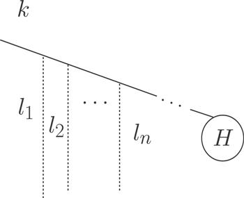
Figure 5. Couplings between Glauber gluons and an active particle, where H represents the hard vertex and dot lines represent Glauber gluons. Other parts of the whole diagram are not displayed explicitly. |
At the leading power of λ and η, we have
$\begin{eqnarray}\begin{array}{l}{\rm{Figure}}\,5=\displaystyle \int \displaystyle \frac{{\rm{d}}{l}_{1}^{-}}{2\pi }\cdots \displaystyle \int \displaystyle \frac{{\rm{d}}{l}_{n}^{-}}{2\pi }\displaystyle \int \displaystyle \frac{{{\rm{d}}}^{D-2}{l}_{1\perp }}{{\left(2\pi \right)}^{D-2}}\cdots \displaystyle \int \displaystyle \frac{{{\rm{d}}}^{D-2}{l}_{n\perp }}{{\left(2\pi \right)}^{D-2}}\\ \quad \times \displaystyle \frac{1}{{k}^{-}+{l}_{1}^{-}\,+\,\tfrac{{\left({k}_{\perp }+{l}_{1\perp }\right)}^{2}}{2{k}^{+}}+{\rm{i}}\varepsilon }\cdots \\ \quad \times \displaystyle \frac{1}{{k}^{-}+{l}_{1}^{-}\,+\cdots +\,{l}_{n}^{-}\,+\,\tfrac{{\left({k}_{\perp }+{l}_{1\perp }\,+\cdots +\,{l}_{n\perp }\right)}^{2}}{2{k}^{+}}+{\rm{i}}\varepsilon }\\ \quad \cdots \displaystyle \frac{1}{{k}^{-}+{l}_{1}^{-}\,+\cdots +\,{l}_{n}^{-}\,+\cdots +\,\tfrac{{\left({k}_{\perp }+{l}_{1\perp }\,+\cdots +\,{l}_{n\perp }+\cdots \right)}^{2}}{2{k}^{+}}+{\rm{i}}\varepsilon }\\ \quad \times \displaystyle \frac{1}{{l}_{1\perp }^{2}+{\rm{i}}\varepsilon }\cdots \displaystyle \frac{1}{{l}_{n\perp }^{2}+{\rm{i}}\varepsilon }\times { \mathcal F }({l}_{1\perp },\ldots ,{l}_{n\perp })\\ \quad \times ({\rm{terms}}\,{\rm{independent}}\,{\rm{of}}\,{l}_{j}^{-}\,{\rm{and}}\,{l}_{j\perp })(1\leqslant j\leqslant n),\end{array}\end{eqnarray}$
where D = 4 − 2ϵ and ${ \mathcal F }({l}_{1\perp },\ldots ,{l}_{n\perp })$ represents the terms on the other ends of these Glauber gluons.One can easily verify that
$\begin{eqnarray}\begin{array}{l}\displaystyle \int \displaystyle \frac{{\rm{d}}{l}_{1}^{-}}{2\pi }\cdots \displaystyle \int \displaystyle \frac{{\rm{d}}{l}_{n}^{-}}{2\pi }\left(\displaystyle \frac{1}{{k}^{-}+{l}_{1}^{-}\,+\,\tfrac{{\left({k}_{\perp }\right)}^{2}}{2{k}^{+}}+{\rm{i}}\varepsilon }\cdots \right.\\ \quad \times \displaystyle \frac{1}{{k}^{-}+{l}_{1}^{-}\,+\cdots +\,{l}_{n}^{-}\,+\cdots +\,\tfrac{{\left({k}_{\perp }+\cdots \right)}^{2}}{2{k}^{+}}+{\rm{i}}\varepsilon }\\ \quad -\displaystyle \frac{1}{{k}^{-}+{l}_{1}^{-}\,+\,\tfrac{{\left({k}_{\perp }+{l}_{1\perp }\right)}^{2}}{2{k}^{+}}+{\rm{i}}\varepsilon }\cdots \\ \quad \left.\times \displaystyle \frac{1}{{k}^{-}+{l}_{1}^{-}\,+\cdots +\,{l}_{n}^{-}\,+\cdots +\,\tfrac{{\left({k}_{\perp }+{l}_{1\perp }\,+\cdots +\,{l}_{n\perp }+\cdots \right)}^{2}}{2{k}^{+}}+{\rm{i}}\varepsilon }\right)\\ \quad =\,0.\end{array}\end{eqnarray}$
Hence $\begin{eqnarray}\begin{array}{l}{\rm{Figure}}\,5=\displaystyle \int \displaystyle \frac{{\rm{d}}{l}_{1}^{-}}{2\pi }\cdots \displaystyle \int \displaystyle \frac{{\rm{d}}{l}_{n}^{-}}{2\pi }\displaystyle \int \displaystyle \frac{{{\rm{d}}}^{D-2}{l}_{1\perp }}{{\left(2\pi \right)}^{D-2}}\cdots \displaystyle \int \displaystyle \frac{{{\rm{d}}}^{D-2}{l}_{n\perp }}{{\left(2\pi \right)}^{D-2}}\\ \quad \times \displaystyle \frac{1}{{k}^{-}+{l}_{1}^{-}\,+\,\tfrac{{\left({k}_{\perp }\right)}^{2}}{2{k}^{+}}+{\rm{i}}\varepsilon }\cdots \\ \quad \times \displaystyle \frac{1}{{k}^{-}+{l}_{1}^{-}\,+\cdots +\,{l}_{n}^{-}\,+\,\tfrac{{\left({k}_{\perp }\right)}^{2}}{2{k}^{+}}+{\rm{i}}\varepsilon }\cdots \\ \quad \times \displaystyle \frac{1}{{k}^{-}+{l}_{1}^{-}\,+\cdots +\,{l}_{n}^{-}\,+\cdots +\,\tfrac{{\left({k}_{\perp }+\cdots \right)}^{2}}{2{k}^{+}}+{\rm{i}}\varepsilon }\\ \quad \times \displaystyle \frac{1}{{l}_{1\perp }^{2}+{\rm{i}}\varepsilon }\cdots \displaystyle \frac{1}{{l}_{n\perp }^{2}+{\rm{i}}\varepsilon }\times { \mathcal F }({l}_{1\perp },\ldots ,{l}_{n\perp })\\ \quad \times ({\rm{terms}}\,{\rm{independent}}\,{\rm{of}}\,{l}_{j}^{-}\,{\rm{and}}\,{l}_{j\perp })(1\leqslant j\leqslant n)\end{array}\end{eqnarray}$
at leading power of λ and η. That is to say, the Glauber of couplings k eikonalize at leading power of λ and η.We then consider active particles which do not couple to the hard vertex directly. We consider a plus-collinear active particle ${k}^{{\prime} }$. ${k}^{{\prime} +}$ is restricted to flow into the hard vertex. We consider Glauber couplings of active particles along the flow of the plus momenta. ${k}^{{\prime} }$ may couple to some Glauber gluons l1,…,ln and other particles q1,…,qm. The momentum of the active particle becomes ${k}^{{\prime} }+{l}_{1}\,+\cdots +\,{l}_{n}+\,{q}_{1}\,+\cdots +\,{q}_{m}$. Finally one meets the hard vertex, which is independent of l1,…,ln. At the leading power of λ and η, these couplings rely on l1,…,ln though the term49 ), we see that the couplings between the Glauber gluons l1,…,ln and the active particle ${k}^{{\prime} }$ eikonalize.
$\begin{eqnarray}\begin{array}{l}\displaystyle \int \displaystyle \frac{{\rm{d}}{l}_{1}^{-}}{2\pi }\cdots \displaystyle \int \displaystyle \frac{{\rm{d}}{l}_{n}^{-}}{2\pi }\displaystyle \int \displaystyle \frac{{{\rm{d}}}^{D-2}{l}_{1\perp }}{{\left(2\pi \right)}^{D-2}}\cdots \\ \quad \times \displaystyle \int \displaystyle \frac{{{\rm{d}}}^{D-2}{l}_{n\perp }}{{\left(2\pi \right)}^{D-2}}\displaystyle \frac{1}{{k}^{{\prime} -}+{l}_{1}^{-}\,+\,\tfrac{{\left({k}_{\perp }+{l}_{1\perp }\right)}^{2}}{2{k}^{{\prime} +}}+{\rm{i}}\varepsilon }\\ \quad \cdots \displaystyle \frac{1}{{k}^{{\prime} -}+{l}_{1}^{-}\,+\cdots +\,{l}_{n}^{-}+{q}_{1}^{-}\,+\cdots +\,{q}_{m}^{-}+\tfrac{{\left({k}_{\perp }+{l}_{1\perp }\,+\cdots +\,{l}_{n\perp }++{q}_{1\perp }\,+\cdots +\,{q}_{m\perp }\right)}^{2}}{2({k}^{{\prime} +}+{q}_{1}^{+}+\cdots +{q}_{m}^{+})}+{\rm{i}}\varepsilon }\\ \quad \times \displaystyle \frac{1}{{l}_{1\perp }^{2}+{\rm{i}}\varepsilon }\cdots \displaystyle \frac{1}{{l}_{n\perp }^{2}+{\rm{i}}\varepsilon }\times { \mathcal F }({l}_{1\perp },\ldots ,{l}_{n\perp })\\ \quad \times ({\rm{terms}}\,{\rm{independent}}\,{\rm{of}}\,{l}_{j}^{-}\,{\rm{and}}\,{l}_{j\perp })(1\leqslant j\leqslant n).\end{array}\end{eqnarray}$
According to similar discussions as those for (For the Glauber couplings of minus-collinear active particles, we have similar results. In conclusion, Glauber couplings of active particles eikonalize at the leading power of λ and η in ${ \mathcal H }(P,\bar{P},{q}^{+},{q}^{-})$.
4.3. Glauber gluons exchanged between active and soft particles
We consider active-soft Glauber exchanges in this section. These Glauber gluons can be absorbed into soft Wilson lines according to discussions here.
Without loss of generality, we consider the Glauber gluons exchanged between plus-collinear active particles and soft particles. To specify our discussions, let us consider the Glauber gluons(l1,…,ln) exchanged between a plus-collinear active particle k and a soft particle ks.
The couplings between k and Glauber gluons read (49 )51 ) with (52 ), we see that Glauber gluons behave like soft gluons while coupling to k.
$\begin{eqnarray}\begin{array}{l}\displaystyle \int \displaystyle \frac{{{\rm{d}}}^{D}{l}_{1}}{{\left(2\pi \right)}^{D}}\cdots \displaystyle \int \displaystyle \frac{{{\rm{d}}}^{D}{l}_{n}}{{\left(2\pi \right)}^{D}}\displaystyle \frac{1}{{k}^{-}+{l}_{1}^{-}\,+\,\tfrac{{\left({k}_{\perp }\right)}^{2}}{2{k}^{+}}+{\rm{i}}\varepsilon }\cdots \\ \quad \times \displaystyle \frac{1}{{k}^{-}+{l}_{1}^{-}\,+\cdots +\,{l}_{n}^{-}\,+\,\tfrac{{\left({k}_{\perp }\right)}^{2}}{2{k}^{+}}+{\rm{i}}\varepsilon }\\ \quad \cdots \displaystyle \frac{1}{{k}^{-}+{l}_{1}^{-}\,+\cdots +\,{l}_{n}^{-}\,+\cdots +\,\tfrac{{\left({k}_{\perp }+\cdots \right)}^{2}}{2{k}^{+}}+{\rm{i}}\varepsilon }\\ \quad \times \displaystyle \frac{1}{{l}_{1\perp }^{2}+{\rm{i}}\varepsilon }\cdots \displaystyle \frac{1}{{l}_{n\perp }^{2}+{\rm{i}}\varepsilon }\\ \quad \times ({\rm{terms}}\,{\rm{independent}}\,{\rm{of}}{l}_{j})(1\leqslant j\leqslant n)\\ \quad \times ({\rm{terms}}\,{\rm{on}}\,{\rm{the}}\,{\rm{other}}\,{\rm{ends}}\,{\rm{of}}{l}_{1},\ldots ,{l}_{n})\end{array}\end{eqnarray}$
at leading power of λ and η, where D = 4 − 2ϵ. We compare the result with the case that k couple to soft gluons q1,…,qn. After the eikonal approximation, the couplings between q1,…,qn and k read $\begin{eqnarray}\begin{array}{l}\displaystyle \int \displaystyle \frac{{{\rm{d}}}^{D}{q}_{1}}{{\left(2\pi \right)}^{D}}\cdots \displaystyle \int \displaystyle \frac{{{\rm{d}}}^{D}{q}_{n}}{{\left(2\pi \right)}^{D}}\displaystyle \frac{1}{{k}^{-}+{q}_{1}^{-}\,+\,\tfrac{{\left({k}_{\perp }\right)}^{2}}{2{k}^{+}}+{\rm{i}}\varepsilon }\cdots \\ \quad \times \displaystyle \frac{1}{{k}^{-}+{q}_{1}^{-}\,+\cdots +\,{q}_{n}^{-}\,+\,\tfrac{{\left({k}_{\perp }\right)}^{2}}{2{k}^{+}}+{\rm{i}}\varepsilon }\\ \quad \cdots \displaystyle \frac{q}{{k}^{-}+{q}_{1}^{-}\,+\cdots +\,{q}_{n}^{-}\,+\cdots +\,\tfrac{{\left({k}_{\perp }+\cdots \right)}^{2}}{2{k}^{+}}+{\rm{i}}\varepsilon }\\ \quad \times \displaystyle \frac{1}{{q}_{1}^{+}{q}_{1}^{-}+{q}_{1\perp }^{2}+{\rm{i}}\varepsilon }\cdots \displaystyle \frac{1}{{q}_{n}^{+}{q}_{n}^{-}+{q}_{n\perp }^{2}+{\rm{i}}\varepsilon }\\ \quad \times ({\rm{terms}}\,{\rm{independent}}\,{\rm{of}}\,{q}_{j})(1\leqslant j\leqslant n)\\ \quad \times ({\rm{terms}}\,{\rm{on}}\,{\rm{the}}\,{\rm{other}}\,{\rm{ends}}\,{\rm{of}}\,{q}_{1},\,\ldots \,,{q}_{n})\end{array}\end{eqnarray}$
at leading power of λ and η. Comparing (l1,…,ln couple to soft particles ks on the other ends. While coupling to soft particles, Glauber gluons behave like soft gluons as demonstrated in the effective action (7 ). In fact, the Glauber region can be viewed as the subregion of the soft region in loop integrals once the Glauber couplings eikonalize. Hence the couplings between Glauber gluons and ks can be absorbed into soft couplings of ks by absorbing the Glauber region into the soft region in loop integrals. In summary, the active-soft type Glauber gluons behave like soft gluons on both ends.
We also notice that the couplings between Glauber gluons and ultrasoft particles are power suppressed according to table 2. So are the couplings between soft gluons and ultrasoft particles. Hence Glauber gluons behave like soft gluons at the leading power of λ while coupling to ultrasoft particles.
In addition, the propagators of lj behave like those of qj in the special momenta region ($| {q}_{j}^{-}| \ll | {q}_{j\perp }| ,\quad 1\leqslant j\leqslant n$).
According to the above facts, we see that Glauber gluons exchanged between ks and k behave like soft gluons and can be absorbed into soft Wilson along +-direction. For other active-soft Glauber exchanges, we have similar results. In other words, active-soft Glauber exchanges can be absorbed into zero bins of soft Wilson lines.15(The Wilson lines should be past pointing according to the poles’ location of ${l}_{j}^{-}$ in (49 ). One may also see this by simply realizing that final interactions cancel out in ${ \mathcal H }(P,\bar{P},{q}^{+},{q}^{-})$ as discussed in section 3.2. )
4.4. Glauber gluons exchanged between spectators and active particles
We consider active-spectator Glauber exchanges in this section. These Glauber gluons are absorbed into collinear Wilson lines according to discussions here.
Without loss of generality, we consider the Glauber gluons exchanged between a minus-collinear spectator $\bar{K}$ and a plus-collinear active particle k(k+ > 0 as plus momenta flow from plus-collinear particles to the hard vertex). While coupling to spectators, these Glauber gluons behave like the collinear gluons ${A}_{-,\bar{p}}^{\mu }$ with ${\bar{p}}^{-}=0$. On the other hand, couplings between Glauber and ultrasoft gluons are power suppressed according to the power counting results in table 2. Hence, we can use the eikonal approximation in couplings between Glauber and ultrasoft gluons without affecting the leading power results. So are couplings between these Glauber gluons and other Glauber gluons.16(Couplings between Glauber and soft gluons are discussed in section 4.4 .) In other words, these Glauber gluons behave like collinear gluons ${A}_{-,\bar{p}}^{\mu }$ with ${\bar{p}}^{-}=0$ while coupling to spectators and ultrasoft and Glauber gluons.
On the other end, these Glauber gluons couple to plus-collinear active particles. According to the results of section 4.2 , such couplings eikonalize at the leading power of λ and η. The couplings between these Glauber gluons and k read (49 )
$\begin{eqnarray}\begin{array}{l}\displaystyle \int \displaystyle \frac{{{\rm{d}}}^{D}{l}_{1}}{{\left(2\pi \right)}^{D}}\cdots \displaystyle \int \displaystyle \frac{{{\rm{d}}}^{D}{l}_{n}}{{\left(2\pi \right)}^{D}}\displaystyle \frac{1}{{k}^{-}+{l}_{1}^{-}\,+\,\tfrac{{\left({k}_{\perp }\right)}^{2}}{2{k}^{+}}+{\rm{i}}\varepsilon }\cdots \\ \quad \times \displaystyle \frac{1}{{k}^{-}+{l}_{1}^{-}\,+\cdots +\,{l}_{n}^{-}\,+\,\tfrac{{\left({k}_{\perp }\right)}^{2}}{2{k}^{+}}+{\rm{i}}\varepsilon }\\ \quad \cdots \displaystyle \frac{1}{{k}^{-}+{l}_{1}^{-}\,+\cdots +\,{l}_{n}^{-}\,+\cdots +\,\tfrac{{\left({k}_{\perp }+\cdots \right)}^{2}}{2{k}^{+}}+{\rm{i}}\varepsilon }\\ \quad \times \displaystyle \frac{1}{{l}_{1\perp }^{2}+{\rm{i}}\varepsilon }\cdots \displaystyle \frac{1}{{l}_{n\perp }^{2}+{\rm{i}}\varepsilon }\\ \quad \times ({\rm{terms}}\,{\rm{independent}}\,{\rm{of}}\,{l}_{j})(1\leqslant j\leqslant n)\\ \quad \times ({\rm{terms}}\,{\rm{on}}\,{\rm{the}}\,{\rm{other}}\,{\rm{ends}}\,{\rm{of}}\,{l}_{1},\ldots ,{l}_{n})\end{array}\end{eqnarray}$
at leading power of λ and η, where D = 4 − 2ϵ. On the other hand, one may consider the couplings between k and minus-collinear gluons. We denote the momenta of these collinear gluons as ${\bar{k}}_{1},\ldots ,{\bar{k}}_{n}$. The couplings between these collinear gluons and k can be written as $\begin{eqnarray}\begin{array}{l}\displaystyle \int \displaystyle \frac{{{\rm{d}}}^{D}{\bar{k}}_{1}}{{\left(2\pi \right)}^{D}}\cdots \displaystyle \int \displaystyle \frac{{{\rm{d}}}^{D}{\bar{k}}_{n}}{{\left(2\pi \right)}^{D}}\displaystyle \frac{1}{{k}^{-}+{\bar{k}}_{1}^{-}\,+\,\tfrac{{\left({k}_{\perp }\right)}^{2}}{2{k}^{+}}+{\rm{i}}\varepsilon }\cdots \\ \quad \times \displaystyle \frac{1}{{k}^{-}+{\bar{k}}_{1}^{-}\,+\cdots +\,{\bar{k}}_{n}^{-}\,+\,\tfrac{{\left({k}_{\perp }\right)}^{2}}{2{k}^{+}}+{\rm{i}}\varepsilon }\\ \quad \cdots \displaystyle \frac{1}{{k}^{-}+{\bar{k}}_{1}^{-}\,+\cdots +\,{\bar{k}}_{n}^{-}\,+\cdots +\,\tfrac{{\left({k}_{\perp }+\cdots \right)}^{2}}{2{k}^{+}}+{\rm{i}}\varepsilon }\\ \quad \times \displaystyle \frac{1}{{\bar{k}}_{1}^{+}{\bar{k}}_{1}^{-}+{\bar{k}}_{1\perp }^{2}+{\rm{i}}\varepsilon }\cdots \displaystyle \frac{1}{{\bar{k}}_{n}^{+}{\bar{k}}_{n}^{-}+{\bar{k}}_{n\perp }^{2}+{\rm{i}}\varepsilon }\\ \quad \times ({\rm{terms}}\,{\rm{independent}}\,{\rm{of}}\,{\bar{k}}_{j})(1\leqslant j\leqslant n)\\ \quad \times ({\rm{terms}}\,{\rm{on}}\,{\rm{the}}\,{\rm{other}}\,{\rm{ends}}\,{\rm{of}}\,{\bar{k}}_{1},\ldots ,{\bar{k}}_{n})\end{array}\end{eqnarray}$
at leading power of λ and η, where we have made use of the eikonal approximation in couplings between k and ${\bar{k}}_{1},\ldots ,{\bar{k}}_{n}$. We see that the couplings between k and l1, …ln behave like those between k and ${\bar{k}}_{1},\ldots ,{\bar{k}}_{n}$.In summary, Glauber gluons exchanged between $\bar{K}$ and k behave like collinear gluons ${A}_{-,\bar{p}}^{\mu }$ with ${\bar{p}}^{-}=0$ on both ends. The propagators of these Glauber gluons behave like those of the collinear gluons ${A}_{-,\bar{p}}^{\mu }$ with ${\bar{p}}^{-}=0$ too. Hence the Glauber gluons exchanged between $\bar{K}$ and k can be absorbed into minus-collinear Wilson lines by extending the collinear region to include the Glauber region in the loop integrals.17(The Wilson lines should be past pointing as final interactions cancel out in ${ \mathcal H }(P,\bar{P},{q}^{+},{q}^{-})$ as discussed in section 3.2 )
For general active-spectator Glauber exchanges, we have similar results. In conclusion, active-spectator Glauber exchanges can be absorbed into collinear Wilson lines.
4.5. Glauber gluons exchanged between active particles
We consider active–active Glauber exchanges in this section. They can be absorbed into soft Wilson lines for ladder diagrams [30]. In this section, we extend the result to the general situation.
Without loss of generality, we consider the Glauber gluons(l1,…,ln) exchanged between a plus-collinear active particle k(k+ > 0 as plus momenta flow from plus-collinear particles to the hard vertex) and a minus-collinear active particle $\bar{k}$(${\bar{k}}^{-}\gt 0$ as minus momenta flow from minus-collinear particles to the hard vertex). Glauber couplings of active particles eikonalize according to the result in section 4.2 . In other words, we can use the eikonal approximation on both ends of these Glauber gluons. The couplings between k and these Glauber gluons can be written as (49 )55 ) with (56 ) and (57 ), we see that the Glauber gluons behave like collinear gluons ${A}_{+,0}^{\mu }$ and soft gluons ${A}_{s}^{\mu }$ while coupling to k.
$\begin{eqnarray}\begin{array}{l}\displaystyle \int \displaystyle \frac{{{\rm{d}}}^{D}{l}_{1}}{{\left(2\pi \right)}^{D}}\cdots \displaystyle \int \displaystyle \frac{{{\rm{d}}}^{D}{l}_{n}}{{\left(2\pi \right)}^{D}}\displaystyle \frac{1}{{k}^{-}+{l}_{1}^{-}\,+\,\tfrac{{\left({k}_{\perp }\right)}^{2}}{2{k}^{+}}+{\rm{i}}\varepsilon }\cdots \\ \quad \times \displaystyle \frac{1}{{k}^{-}+{l}_{1}^{-}\,+\cdots +\,{l}_{n}^{-}\,+\,\tfrac{{\left({k}_{\perp }\right)}^{2}}{2{k}^{+}}+{\rm{i}}\varepsilon }\\ \quad \cdots \displaystyle \frac{1}{{k}^{-}+{l}_{1}^{-}\,+\cdots +\,{l}_{n}^{-}\,+\cdots +\,\tfrac{{\left({k}_{\perp }+\cdots \right)}^{2}}{2{k}^{+}}+{\rm{i}}\varepsilon }\\ \quad \times \displaystyle \frac{1}{{l}_{1\perp }^{2}+{\rm{i}}\varepsilon }\cdots \displaystyle \frac{1}{{l}_{n\perp }^{2}+{\rm{i}}\varepsilon }\\ \quad \times ({\rm{terms}}\,{\rm{independent}}\,{\rm{of}}\,{l}_{j})(1\leqslant j\leqslant n)\\ \quad \times ({\rm{terms}}\,{\rm{on}}\,{\rm{the}}\,{\rm{other}}\,{\rm{ends}}\,{\rm{of}}\,{l}_{1},\ldots ,{l}_{n})\end{array}\end{eqnarray}$
at leading power of λ and η, where D = 4 − 2ϵ. One may compare the result with the cases that k couple to minus-collinear gluons ${\bar{p}}_{1},\ldots ,{\bar{p}}_{n}$ or soft gluons q1,…,qn. After the eikonal approximation, the couplings between ${\bar{p}}_{1},\ldots ,{\bar{p}}_{n}$ and k read $\begin{eqnarray}\begin{array}{l}\displaystyle \int \displaystyle \frac{{{\rm{d}}}^{D}{\bar{p}}_{1}}{{\left(2\pi \right)}^{D}}\cdots \displaystyle \int \displaystyle \frac{{{\rm{d}}}^{D}{\bar{p}}_{n}}{{\left(2\pi \right)}^{D}}\displaystyle \frac{1}{{k}^{-}+{\bar{p}}_{1}^{-}\,+\,\tfrac{{\left({k}_{\perp }\right)}^{2}}{2{k}^{+}}+{\rm{i}}\varepsilon }\cdots \\ \quad \times \displaystyle \frac{1}{{k}^{-}+{\bar{p}}_{1}^{-}\,+\cdots +\,{\bar{p}}_{n}^{-}\,+\,\tfrac{{\left({k}_{\perp }\right)}^{2}}{2{k}^{+}}+{\rm{i}}\varepsilon }\\ \quad \cdots \displaystyle \frac{1}{{k}^{-}+{\bar{p}}_{1}^{-}\,+\cdots +\,{\bar{p}}_{n}^{-}\,+\cdots +\,\tfrac{{\left({k}_{\perp }+\cdots \right)}^{2}}{2{k}^{+}}+{\rm{i}}\varepsilon }\\ \quad \times \displaystyle \frac{1}{{\bar{p}}_{1}^{+}{\bar{p}}_{1}^{-}+{\bar{p}}_{1\perp }^{2}+{\rm{i}}\varepsilon }\cdots \displaystyle \frac{1}{{\bar{p}}_{n}^{+}{\bar{p}}_{n}^{-}+{\bar{p}}_{n\perp }^{2}+{\rm{i}}\varepsilon }\\ \quad \times ({\rm{terms}}\,{\rm{independent}}\,{\rm{of}}\,{\bar{p}}_{j})(1\leqslant j\leqslant n)\\ \quad \times ({\rm{terms}}\,{\rm{on}}\,{\rm{the}}\,{\rm{other}}\,{\rm{ends}}\,{\rm{of}}\,{\bar{p}}_{1},\ldots ,{\bar{p}}_{n})\end{array}\end{eqnarray}$
and the couplings between q1,…,qn and k read $\begin{eqnarray}\begin{array}{l}\displaystyle \int \displaystyle \frac{{{\rm{d}}}^{D}{q}_{1}}{{\left(2\pi \right)}^{D}}\cdots \displaystyle \int \displaystyle \frac{{{\rm{d}}}^{D}{q}_{n}}{{\left(2\pi \right)}^{D}}\displaystyle \frac{1}{{k}^{-}+{q}_{1}^{-}\,+\,\tfrac{{\left({k}_{\perp }\right)}^{2}}{2{k}^{+}}+{\rm{i}}\varepsilon }\cdots \\ \quad \times \displaystyle \frac{1}{{k}^{-}+{q}_{1}^{-}\,+\cdots +\,{q}_{n}^{-}\,+\,\tfrac{{\left({k}_{\perp }\right)}^{2}}{2{k}^{+}}+{\rm{i}}\varepsilon }\cdots \\ \quad \times \displaystyle \frac{1}{{k}^{-}+{q}_{1}^{-}\,+\cdots +\,{q}_{n}^{-}\,+\cdots +\,\tfrac{{\left({k}_{\perp }+\cdots \right)}^{2}}{2{k}^{+}}+{\rm{i}}\varepsilon }\\ \quad \times \displaystyle \frac{1}{{q}_{1}^{+}{q}_{1}^{-}+{q}_{1\perp }^{2}+{\rm{i}}\varepsilon }\cdots \displaystyle \frac{1}{{q}_{n}^{+}{q}_{n}^{-}+{q}_{n\perp }^{2}+{\rm{i}}\varepsilon }\\ \quad \times ({\rm{terms}}\,{\rm{independent}}\,{\rm{of}}\,{q}_{j})(1\leqslant j\leqslant n)\\ \quad \times ({\rm{terms}}\,{\rm{on}}\,{\rm{the}}\,{\rm{other}}\,{\rm{ends}}\,{\rm{of}}\,{q}_{1},\ldots ,{q}_{n})\end{array}\end{eqnarray}$
at leading power of λ and η. Comparing (For the couplings between l1,…,ln and $\bar{k}$, we have a similar result and the Glauber gluons behave like collinear gluons ${A}_{-,0}^{\mu }$ and soft gluons ${A}_{s}^{\mu }$ in these couplings.
According to the above discussions, we see that Glauber gluons exchanged between k and $\bar{k}$ behave like soft gluons on both ends. In addition, the propagators of l1,…,ln behave like those of q1,…,qn in the special momenta region($| {q}_{j}^{+}| \ll | {q}_{j\perp }| $, $| {q}_{j}^{-}| \ll | {q}_{j\perp }| $).
For general active–active Glauber exchanges, we have similar results. Hence active–active Glauber exchanges can be absorbed into soft Wilson lines by extending the soft region to include the Glauber region in loop integrals.18(These Wilson lines should be past pointing as final interactions cancel out in ${ \mathcal H }(P,\bar{P},{q}^{+},{q}^{-})$.)
5. Cancellation of spectator–spectator and spectator-soft Glauber exchanges in ${ \mathcal H }(P,\bar{P},{q}^{+},{q}^{-})$
In this section, we prove the cancellation of the spectator–spectator and the spectator-soft Glauber exchanges in ${ \mathcal H }(P,\bar{P},{q}^{+},{q}^{-})$ 19(Soft–soft Glauber exchanges are power stressed and can be absorbed into soft exchanges between soft particles.). Calculations in [30] show the cancellation of the spectator–spectator type Glauber exchanges in ladder diagrams. According to our discussions in section 3.1 , ladder diagrams of Glauber gluons exchanged between spectators in ${ \mathcal H }$ can be understood as perturbative series of the object3.1 . In this case, the summation over all possible spectator states is not obstructed by the coherence and the cancellation of the ladder diagrams is the direct result of the unitarity of the time evolution of spectators. That is, cancellation occurs between interactions in the evolution and the conjugation of the evolution of spectators.
$\begin{eqnarray}\begin{array}{l}\sum _{X}\langle {p}_{1}^{{\prime} }{\bar{p}}_{1}^{{\prime} }\ldots | {U}^{\dagger }(\infty ,-\infty )| X\rangle \langle X| U(\infty ,-\infty )| {p}_{1}{\bar{p}}_{1}\ldots \rangle \\ \quad =\langle {p}_{1}^{{\prime} }{\bar{p}}_{1}^{{\prime} }\ldots | {U}^{\dagger }(\infty ,-\infty )U(\infty ,-\infty )| {p}_{1}{\bar{p}}_{1}\ldots \rangle \\ \quad =\langle {p}_{1}^{{\prime} }{\bar{p}}_{1}^{{\prime} }\ldots | {p}_{1}{\bar{p}}_{1}\ldots \rangle ,\end{array}\end{eqnarray}$
where $| {p}_{1}{\bar{p}}_{1}\ldots \rangle $ and $| {p}_{1}^{{\prime} }{\bar{p}}_{1}^{{\prime} }\ldots \rangle $ represent initial spectators and ∣X⟩ represents possible final states and U(t2, t1) represents the time evolution operator corresponding to the spectator–spectator Glauber exchanges. We have made use of the unitarity of the time evolution operator in the above equation. In fact, the spectator–spectator type Glauber ladder diagrams can be viewed as the possible evolution of spectators. While neglecting active-spectator coherence, the evolutions of active particles and spectators are independent of each other according to discussions in section In general cases, the active-spectator coherence may obstruct the summation over all possible final spectators. For example, one may consider the diagram shown in figure 6.
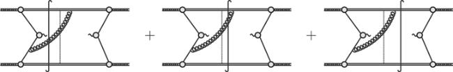
Figure 6. An example of diagrams with the active-spectator coherence which obstructs the summation over all possible Glauber interactions between spectators, where the dot lines represent the Glauber gluons. |
The gluon exchanged between spectators and active particles should not be collinear in the first two diagrams. Otherwise the two diagrams do not contribute to the process considered here. In other words, the summation over Glauber interactions of spectators is hampered by the active-spectator coherence in figure 6. One should deal with the active-spectator coherence carefully to get the cancellation of spectator-spectator and spectator-soft Glauber exchanges.
If the Glauber interactions occur after the spectator-active and the soft-active interactions like the first diagram in figure 7 then the summation over all states after the spectator-active and the soft-active interactions is inclusive enough for the spectator–spectator and the spectator-soft Glauber exchanges.
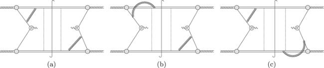
Figure 7. (a) An example of diagrams with the Glauber gluons A+G couple to spectators after the non-Glauber couplings. (b)An example of diagrams with the Glauber gluons A+G couple to plus-collinear spectators before non-Glauber couplings. (c)An example of diagrams with the Glauber gluons A+G couple to minus-collinear spectators before non-Glauber couplings. The Glauber gluons are represented by dot lines in these diagrams. |
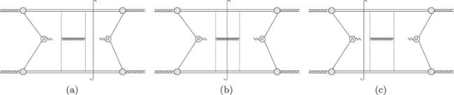
Figure 8. Some examples of spectator–spectator ladder diagrams with soft gluons connecting different ladders. |
The cancellation (58 ) can be extended into this case even if there are spectator-active and soft-active interactions. It seems important for us to exclude spectator-active and soft-active interactions after spectator–spectator and spectator-soft Glauber exchanges like those in figure 6. However, instated of the time evolution of collinear and soft states, we find it convenient to consider the evolution of these states along a nearly light-like direction. This is displayed explicitly in the following sections.
According to the discussions in section 4 , Glauber gluons coupling to active particles should be absorbed into zero bins of collinear or soft gluons. Hence we view Glauber interactions of active particles as collinear or soft interactions of these particles. While referring to Glauber interactions, we always mean the spectator–spectator and the spectator-soft Glauber exchanges in the following texts.
5.1. $\widetilde{{n}_{+}}\cdot x$-evolution in ${ \mathcal H }(P,\bar{P},{q}^{+},{q}^{-})$
It is convenient to consider the x+(or x−)-evolution instead of the time evolution of states in ${ \mathcal H }(P,\bar{P},{q}^{+},{q}^{-})$. Such evolution is crucial in proofs of the factorization theorem of Drell–Yan process in perturbative QCD [4]. In this section, we consider a time-like evolution that is approximately equivalent to x+(or x−)-evolution.
Let us bring in a time-like direction $\widetilde{{n}_{+}}$ and a space-like direction $\widehat{{n}_{+}}$ at first
$\begin{eqnarray}\begin{array}{rcl}{\widetilde{{n}_{+}}}^{\mu } & \equiv & \left({\widetilde{{n}_{+}}}^{+},{\widetilde{{n}_{+}}}^{-},{\widetilde{{n}_{+}}}_{\perp }^{\mu }\right)\equiv \displaystyle \frac{1}{\sqrt{2}}\left(\displaystyle \frac{1}{\sqrt{\lambda \omega }},\sqrt{\lambda \omega },0\right)\\ {\widehat{{n}_{+}}}^{\mu } & \equiv & \left({\widehat{{n}_{+}}}^{+},{\widehat{{n}_{+}}}^{-},{\widetilde{{n}_{+}}}_{\perp }^{\mu }\right)\equiv \displaystyle \frac{1}{\sqrt{2}}\left(\displaystyle \frac{1}{\sqrt{\lambda \omega }},-\sqrt{\lambda \omega },0\right),\end{array}\end{eqnarray}$
where ω is a positive constant of order 1. We have $\begin{eqnarray}\begin{array}{rcl}{\widetilde{{n}_{+}}}^{2} & = & 1,\displaystyle \frac{{\widetilde{{n}_{+}}}^{-}}{{\widetilde{{n}_{+}}}^{+}}=\lambda \omega \\ {\widehat{{n}_{+}}}^{2} & = & -1,\displaystyle \frac{{\widehat{{n}_{+}}}^{-}}{{\widehat{{n}_{+}}}^{+}}=-\lambda \omega .\end{array}\end{eqnarray}$
That is to say $\widetilde{{n}_{+}}$($\widehat{{n}_{+}}$) is time-like (space-like) and nearly collinear to the plus direction.One can choose a reference system so that3.2 one has
$\begin{eqnarray}{\widetilde{{n}_{+}}}^{\mu }\equiv ({\widetilde{{n}_{+}}}^{0},\vec{\widetilde{{n}_{+}}})\to (1,\vec{0})\end{eqnarray}$
in the new reference system. According to the skills in section $\begin{eqnarray}\begin{array}{l}\sum _{X}\displaystyle \int {{\rm{d}}}^{4}{x}_{1}\displaystyle \int {{\rm{d}}}^{4}{x}_{2}\displaystyle \int {{\rm{d}}}^{4}{x}_{3}\displaystyle \int {{\rm{d}}}^{4}{x}_{4}\displaystyle \int {{\rm{d}}}^{4}z{{\rm{e}}}^{{\rm{i}}q\cdot z}\\ \quad \times \left\langle {H}_{1}{H}_{2}| \bar{T}\{{{ \mathcal O }}^{\dagger }({x}_{1}){\bar{{ \mathcal O }}}^{\dagger }({x}_{2}){J}^{\dagger }(z){U}^{\dagger }(\infty ,-\infty )\}| H(q)X\right\rangle \\ \quad \times \left\langle H(q)X| T\{{ \mathcal O }({x}_{3})\bar{{ \mathcal O }}({x}_{4})J(0)U(\infty ,-\infty )\}| {H}_{1}{H}_{2}\right\rangle \\ \quad =\sum _{X}\displaystyle \int {{\rm{d}}}^{4}{x}_{1}\displaystyle \int {{\rm{d}}}^{4}{x}_{2}\displaystyle \int {{\rm{d}}}^{4}{x}_{3}\displaystyle \int {{\rm{d}}}^{4}{x}_{4}\displaystyle \int {{\rm{d}}}^{4}z{{\rm{e}}}^{{\rm{i}}q\cdot z}\\ \quad \times \left\langle {H}_{1}{H}_{2}| {{ \mathcal O }}^{\dagger }({x}_{1}){\bar{{ \mathcal O }}}^{\dagger }({x}_{2})\bar{T}\{{J}^{\dagger }(z){U}^{\dagger }\right.\\ \quad \left.\times (\max \{\widetilde{{n}_{+}}\cdot z,0\},-\infty )\}| H(q)X\right\rangle \\ \quad \times \left\langle H(q)X| T\{J(0)U(\max \{\widetilde{{n}_{+}}\cdot z,0\},-\infty )\}{ \mathcal O }\right.\\ \quad \left.\times ({x}_{3})\bar{{ \mathcal O }}({x}_{4})| {H}_{1}{H}_{2}\right\rangle \end{array}\end{eqnarray}$
in the new reference system.According to the Lorentz invariance of QCD, one has
$\begin{eqnarray}\begin{array}{l}{ \mathcal H }(P,\bar{P},{q}^{+},{q}^{-})\\ \quad \equiv \displaystyle \int \displaystyle \frac{{{\rm{d}}}^{2}{q}_{\perp }}{{\left(2\pi \right)}^{2}}\sum _{X}\displaystyle \int {{\rm{d}}}^{4}{x}_{1}\displaystyle \int {{\rm{d}}}^{4}{x}_{2}\displaystyle \int {{\rm{d}}}^{4}{x}_{3}\displaystyle \int {{\rm{d}}}^{4}{x}_{4}\displaystyle \int {{\rm{d}}}^{4}z{{\rm{e}}}^{{\rm{i}}q\cdot z}\\ \quad \times \left\langle P\bar{P}| {{ \mathcal O }}^{\dagger }({x}_{1}){\bar{{ \mathcal O }}}^{\dagger }({x}_{2})\bar{T}\{{J}^{\dagger }(z){U}_{\widetilde{{n}_{+}}}^{\dagger }\right.\\ \quad \left.\times (\max \{\widetilde{{n}_{+}}\cdot z,0\},-\infty )\}| H(q)X\right\rangle \\ \quad \times \left\langle H(q)X| T\{J(0){U}_{\widetilde{{n}_{+}}}(\max \{\widetilde{{n}_{+}}\cdot z,0\},-\infty ))\}{ \mathcal O }\right.\\ \quad \left.\times ({x}_{3})\bar{{ \mathcal O }}({x}_{4})| P\bar{P}\right\rangle \end{array}\end{eqnarray}$
in the center of mass frame of initial hadrons, where ${U}_{\widetilde{{n}_{+}}}$ represents the evolution operator along the $\widetilde{{n}_{+}}\cdot x$ direction. That is to say, interactions with the coordinates $\widetilde{{n}_{+}}\cdot x$ greater than that of the hard collision cancel out in ${ \mathcal H }(P,\bar{P},{q}^{+},{q}^{-})$.20(One may try to consider the evolution of states along the plus or minus direction directly in ${ \mathcal H }(P,\bar{P},{q}^{+},{q}^{-})$. However, the asymptotic condition in the limit x+ → ∞ or x− → ∞ is not clear to us.)5.2. Couplings involving Glauber gluons A+G in ${ \mathcal H }(P,\bar{P},{q}^{+},{q}^{-})$
In this section, we consider the Glauber gluons A+G exchanged between plus-collinear and other particles. We prove the cancellation of the Glauber couplings at vertexes of which the coordinates $\widetilde{{n}_{+}}\cdot x$ are smaller than those of some vertexes free from A+G (except for the hard vertex).
To distinguish vertexes involving A+G from others, we denote the coordinates of couplings between A+G and plus-collinear particles as yi and those between A+G and minus-collinear and soft particles as ${y}_{i}^{{\prime} }$ and those free from A+G as zi(i = 1, …). Without loss of generality, we consider a Glauber gluon l1 exchanged between the two vertexes y1 and ${y}_{1}^{{\prime} }$. ${l}_{1}^{+}$(${l}_{1}^{-}$) can be neglected at the vertex y1 (${y}_{1}^{{\prime} }$).21(${l}_{1}^{+}\lesssim O$ (Qλ) ≪ p+ ∼ O(Q) and ${l}_{1}^{-}\sim O$ $(Q{\lambda }^{2})\ll {l}_{s}^{-}\sim O$ $(Q\lambda )\ll {\bar{p}}^{-}\sim O(Q)$, where p+ represents the plus momenta of plus-collinear particles and ${l}_{s}^{-}$ and ${\bar{p}}^{-}$ represent the minus momenta of soft and minus-collinear particles.)
The propagator of l1 is independent of ${l}_{1}^{+}$ and ${l}_{1}^{-}$ at the leading power of λ and η. As a result, ${ \mathcal H }(P,\bar{P},{q}^{+},{q}^{-})$ relies on ${l}_{1}^{+}$ and ${l}_{1}^{-}$ only through the term
$\begin{eqnarray}\exp \left(-{\rm{i}}{l}_{1}^{-}{y}_{1}^{+}\,+\,{\rm{i}}{l}_{1}^{+}{y}_{1}^{{\prime} -}\right)\end{eqnarray}$
and the integrals over ${l}_{1}^{-}$ and ${l}_{1}^{+}$ read $\begin{eqnarray}\int \displaystyle \frac{{\rm{d}}{l}_{1}^{-}}{2\pi }\displaystyle \frac{{\rm{d}}{l}_{1}^{+}}{2\pi }\exp \left(-{\rm{i}}{l}_{1}^{-}{y}_{1}^{+}\,+\,{\rm{i}}{l}_{1}^{+}{y}_{1}^{{\prime} -}\right)=\delta ({y}_{1}^{+})\delta ({y}_{1}^{{\prime} -})\end{eqnarray}$
The vertex y1 and the hard vertex are connected through plus-collinear particles. For a plus-collinear particle with momenta ξP + k(ξ ∼ O(1), kμ ≲ Qλ for plus-collinear external lines), the propagator reads
$\begin{eqnarray}\int \displaystyle \frac{{{\rm{d}}}^{4}k}{{\left(2\pi \right)}^{4}}\displaystyle \frac{N(P)}{2\xi {P}^{+}{k}^{-}+{\left({k}_{\perp }\right)}^{2}+{\rm{i}}\varepsilon }{{\rm{e}}}^{-{\rm{i}}k\cdot ({x}_{1}-{x}_{2})}\propto \delta ({x}_{1}^{-}-{x}_{2}^{-}),\end{eqnarray}$
where N(P) represents possible numerators in the propagators.We have
$\begin{eqnarray}{y}_{1}^{-}=0,\quad \delta ({y}_{1}^{+})=\sqrt{\displaystyle \frac{\lambda \omega }{2}}\delta \left(\widetilde{{n}_{+}}\cdot {y}_{1}\right)\end{eqnarray}$
on the left side of the final cut and $\begin{eqnarray}{y}_{1}^{-}\,=\,{z}^{-},\quad \delta ({y}_{1}^{+})\simeq \delta ({y}_{1}^{+}-{z}^{+})=\sqrt{\displaystyle \frac{\lambda \omega }{2}}\delta \left(\widetilde{{n}_{+}}\cdot {y}_{1}-\widetilde{{n}_{+}}\cdot z\right)\end{eqnarray}$
on the right side of the final cut, where we have made use of the fact $\begin{eqnarray}{z}^{+}\sim {z}^{-}\sim 1/Q.\end{eqnarray}$
For the vertex ${y}_{1}^{{\prime} }$, we have
$\begin{eqnarray}\delta ({y}_{1}^{{\prime} -})\simeq \displaystyle \frac{1}{\sqrt{2\lambda \omega }}\delta \left(\widetilde{{n}_{+}}\cdot {y}_{1}^{{\prime} }\right)\end{eqnarray}$
on the left side of the final cut and $\begin{eqnarray}\delta ({y}_{1}^{{\prime} -})\simeq \delta ({y}_{1}^{{\prime} -}-{z}_{1}^{-})\simeq \displaystyle \frac{1}{\sqrt{2\lambda \omega }}\delta \left(\widetilde{{n}_{+}}\cdot {y}_{1}^{{\prime} }-\widetilde{{n}_{+}}\cdot {y}_{1}\right)\end{eqnarray}$
on the right side of the final cut. Hence $\begin{eqnarray}\widetilde{{n}_{+}}\cdot {z}_{i}\leqslant 0\Rightarrow \widetilde{{n}_{+}}\cdot {z}_{i}\leqslant \widetilde{{n}_{+}}\cdot {y}_{1},\quad \widetilde{{n}_{+}}\cdot {z}_{i}\leqslant \widetilde{{n}_{+}}\cdot {y}_{1}^{{\prime} }\end{eqnarray}$
on the left side of the final cut and $\begin{eqnarray}\widetilde{{n}_{+}}\cdot {z}_{i}\leqslant \widetilde{{n}_{+}}\cdot z\Rightarrow \widetilde{{n}_{+}}\cdot {z}_{i}\leqslant \widetilde{{n}_{+}}\cdot {y}_{1},\quad \widetilde{{n}_{+}}\cdot {z}_{i}\leqslant \widetilde{{n}_{+}}\cdot {y}_{1}^{{\prime} }\end{eqnarray}$
on the right side of the final cut. That is to say $\begin{eqnarray}\widetilde{{n}_{+}}\cdot {z}_{i}\leqslant \widetilde{{n}_{+}}\cdot {y}_{1},\quad \widetilde{{n}_{+}}\cdot {z}_{i}\leqslant \widetilde{{n}_{+}}\cdot {y}_{1}^{{\prime} }\end{eqnarray}$
on both sides of the final cut.For other vertexes involving the Glauber gluons A+G, we repeat the calculations and get similar results. We conclude that the Glauber gluons A+G should couple to collinear or soft particles at vertexes with coordinates $\widetilde{{n}_{+}}\cdot {y}_{i}$ greater than those of vertexes free from A+G(except for the hard vertex), otherwise effects of the Glauber gluons A+G cancel out at leading power of λ and η.
5.3. Cancellation of Glauber gluon A+G
In this section, we prove the cancellation of the Glauber gluons A+G, which are exchanged between plus-collinear and minus-collinear spectators or between plus-collinear spectators and soft particles.
According to the results of section 5.2 , the Glauber gluons A+G should couple to collinear and soft particles at vertexes with the coordinates $\widetilde{{n}_{+}}\cdot x$ greater than those of vertexes free from A+G(except for vertexes in the hard subprocess). After the absorption of Glauber gluons coupling to active particles into collinear and soft Wilson lines, we have7 ) and
$\begin{aligned}& \mathcal{H}\left(P, \bar{P}, q^{+}, q^{-}\right) \\\equiv & \int \frac{\mathrm{d}^{2} q_{\perp}}{(2 \pi)^{2}} \sum_{X} \int \mathrm{d}^{4} z \mathrm{e}^{\mathrm{i} q \cdot z}\left\langle P \bar{P}\left|\bar{T} \mathcal{O}^{\dagger}\left(S_{+}, S_{-}, W_{+}, W_{-}\right)(x)\right| X\right\rangle \\& \times\left\langle X\left|T\left\{\mathcal{O}\left(S_{+}, S_{-}, W_{+}, W_{-}\right)(0)\right\}\right| P \bar{P}\right\rangle \otimes h(z),\end{aligned}$
where h(z) represents contributions of the hard scattering subprocess and ${ \mathcal O }({S}_{+},{S}_{-},{W}_{+},{W}_{-})$ represents the Wilson line structure of the hard vertex and $\begin{eqnarray}\begin{array}{rcl}{W}_{+}(x) & = & P\exp ({\rm{i}}g{\displaystyle \int }_{-\infty }^{0}{\rm{d}}{{sA}}_{+}^{+}(0,{x}^{-}+s,0)\\ {S}_{+}(x) & = & P\exp ({\rm{i}}g{\displaystyle \int }_{-\infty }^{0}{\rm{d}}s\cdot {A}_{s}^{-}({x}^{+}+s,0,0)\\ {W}_{-}(x) & = & P\exp ({\rm{i}}g{\displaystyle \int }_{-\infty }^{0}{\rm{d}}s\cdot {A}_{-}^{-}({x}^{+}+s,0,0)\\ {S}_{-}(x) & = & P\exp ({\rm{i}}g{\displaystyle \int }_{-\infty }^{0}{\rm{d}}s\cdot {A}_{s}^{+}(0,{x}^{-}+s,0).\end{array}\end{eqnarray}$
The $\widetilde{{n}_{+}}\cdot x$-evolution of these Wilson lines is determined by the operator $\begin{eqnarray}{U}_{{{SCET}}_{G}}(\widetilde{{n}_{+}}\cdot {x}_{1},\widetilde{{n}_{+}}\cdot {x}_{2}),\end{eqnarray}$
where ${U}_{{{SCET}}_{G}}$ represents the n · x evolution operator related to the action ( $\begin{eqnarray}\begin{array}{rcl}{A}^{\mu }(x) & = & {U}_{{{SCET}}_{G}}(\widetilde{{n}_{+}}\cdot x,0){A}^{\mu }(0,\widehat{{n}_{+}}\cdot x,{x}_{\perp }){U}_{{{SCET}}_{G}}^{\dagger }\\ & & \times (\widetilde{{n}_{+}}\cdot x,0)\end{array}\end{eqnarray}$
with ${A}^{\mu }={A}_{+}^{\mu },{A}_{-}^{\mu },{A}_{s}^{\mu }$.According to the results of section 5.2 , A+G couple to spectators and soft particles at vertexes with the coordinates n · x greater than those of vertexes free from A+G in the matrix elements7 ). We show some examples of these diagrams in figure 8. Effects of these diagrams should be absorbed into U+G once they do not bring in active-spectator coherence with the coordinates $\widetilde{{n}_{+}}\cdot x$ greater than those of the hard collision. Otherwise the diagrams can be simply neglected according to discussions in section 5.2 .)
$\begin{eqnarray}\left\langle X| T\{{ \mathcal O }({S}_{+},{S}_{-},{W}_{+},{W}_{-})(0)\}| P\bar{P}\right\rangle \end{eqnarray}$
and $\begin{eqnarray}\left\langle P\bar{P}| \bar{T}{{ \mathcal O }}^{\dagger }({S}_{+},{S}_{-},{W}_{+},{W}_{-})(x)| X\right\rangle .\end{eqnarray}$
We make the perturbative expansion about interactions free from A+G and have $\begin{eqnarray}\begin{array}{l}{ \mathcal H }(P,\bar{P},{q}^{+},{q}^{-})\\ \quad =\sum _{{m}_{1},{m}_{2}}\displaystyle \int \displaystyle \frac{{{\rm{d}}}^{2}{q}_{\perp }}{{\left(2\pi \right)}^{2}}\sum _{X}\displaystyle \int {{\rm{d}}}^{4}z{\displaystyle \int }_{-\infty }^{\widetilde{{n}_{+}}\cdot z}{\rm{d}}{s}_{1}{\displaystyle \int }_{-\infty }^{0}{\rm{d}}{s}_{2}{{\rm{e}}}^{{\rm{i}}q\cdot z}\\ \quad \times \left\langle P\bar{P}| {{ \mathcal O }}_{{m}_{1}}^{\dagger }({s}_{1}){U}_{+G}^{\dagger }(\widetilde{{n}_{+}}\cdot z,{s}_{1})| X\right\rangle \\ \quad \times \left\langle X| {U}_{+G}(0,{s}_{2}){{ \mathcal O }}_{{m}_{2}}({s}_{2})| P\bar{P}\right\rangle \otimes h(z),\end{array}\end{eqnarray}$
where ${{ \mathcal O }}_{{m}_{1}}^{\dagger }$ and ${{ \mathcal O }}_{{m}_{2}}$ represent the m1th and m2th perturbative order interactions free from A+G and U+G represents the $\widetilde{{n}_{+}}\cdot x$ evolution operator corresponding to the spectator–spectator and spectator-soft Glauber exchanges.22(There could be spectator–spectator ladder diagrams with soft gluons connecting different ladders induced by soft-Glauber couplings in the effective action (Considering that5.2 , we have
$\begin{eqnarray}\widetilde{{n}_{+}}\cdot x\simeq 0,\quad \widetilde{{n}_{+}}\cdot z\end{eqnarray}$
for interactions involving the Glauber gluons A+G23(While considering the next leading power results, one has $\widetilde{{n}_{+}}\cdot x\sim O(\lambda )$ and $\widetilde{{n}_{+}}\cdot x\lt 0,\quad \widetilde{{n}_{+}}\cdot x\lt \widetilde{{n}_{+}}\cdot z$.) as discussed in section $\begin{eqnarray}{U}_{+G}(0,{s}_{2})\simeq {U}_{+G}(\infty ,-\infty )\end{eqnarray}$
on the left side of the final cut and $\begin{eqnarray}{U}_{+G}^{\dagger }(\widetilde{{n}_{+}}\cdot z,{s}_{1})\simeq {U}_{+G}^{\dagger }(\infty ,-\infty )\end{eqnarray}$
on the right side of the final cut. Hence $\begin{eqnarray}\begin{array}{l}{ \mathcal H }(P,\bar{P},{q}^{+},{q}^{-})\\ \quad \simeq \sum _{{m}_{1},{m}_{2}}\displaystyle \int \displaystyle \frac{{{\rm{d}}}^{2}{q}_{\perp }}{{\left(2\pi \right)}^{2}}\sum _{X}\displaystyle \int {{\rm{d}}}^{4}z{\displaystyle \int }_{-\infty }^{\widetilde{{n}_{+}}\cdot z}{\rm{d}}{s}_{1}{\displaystyle \int }_{-\infty }^{0}{\rm{d}}{s}_{2}{{\rm{e}}}^{{\rm{i}}q\cdot z}\\ \quad \times \left\langle P\bar{P}| {{ \mathcal O }}_{{m}_{1}}^{\dagger }({s}_{1}){U}_{+G}^{\dagger }(\infty ,-\infty )| X\right\rangle \\ \quad \times \left\langle X| {U}_{+G}(\infty ,-\infty ){{ \mathcal O }}_{{m}_{2}}({s}_{2})| P\bar{P}\right\rangle \otimes h(z)\\ \quad =\sum _{{m}_{1},{m}_{2}}\displaystyle \int \displaystyle \frac{{{\rm{d}}}^{2}{q}_{\perp }}{{\left(2\pi \right)}^{2}}\sum _{X}\displaystyle \int {{\rm{d}}}^{4}z{\displaystyle \int }_{-\infty }^{\widetilde{{n}_{+}}\cdot z}{\rm{d}}{s}_{1}{\displaystyle \int }_{-\infty }^{0}{\rm{d}}{s}_{2}{{\rm{e}}}^{{\rm{i}}q\cdot z}\\ \quad \times \left\langle P\bar{P}| {{ \mathcal O }}_{{m}_{1}}^{\dagger }({s}_{1})| X\right\rangle \left\langle X| {{ \mathcal O }}_{{m}_{2}}({s}_{2})| P\bar{P}\right\rangle \otimes h(z)\end{array}\end{eqnarray}$
at leading power of λ and η. That is, the spectator–spectator and spectator-soft type Glauber exchanges of A+G cancel out in ${ \mathcal H }(P,\bar{P},{q}^{+},{q}^{-})$. We emphasize that the cancellation originates from the unitarity of the $\widetilde{{n}_{+}}\cdot x$ evolution operator induced by interactions between spectators and soft particles. Hence, such cancellation is independent of the details of these interactions.5.4. Cancellation of Glauber gluons A−G
In this section, we consider the Glauber gluons A−G and outline the proof of cancellation of A−G.
According to the results of sections 4 and 5.3 , contributions of A+G can be absorbed into those of collinear gluons A+G and soft gluons As. Hence We can drop the Glauber gluons A+G in calculations of ${ \mathcal H }(P,\bar{P},{q}^{+},{q}^{-})$. After this, we consider the $\widetilde{{n}_{-}}\cdot x$-evolution, where the direction ${\widetilde{{n}_{-}}}^{\mu }$ is defined as5.1 , interactions with the coordinates $\widetilde{{n}_{-}}\cdot x$ greater than those of the hard collision cancel out in ${ \mathcal H }(P,\bar{P},{q}^{+},{q}^{-})$. We have
$\begin{eqnarray}{\widetilde{{n}_{-}}}^{\mu }\equiv ({\widetilde{{n}_{-}}}^{+},{\widetilde{{n}_{-}}}^{-},{\widetilde{{n}_{-}}}_{\perp }^{\mu })\equiv \displaystyle \frac{1}{\sqrt{2}}(\sqrt{\lambda \omega },\displaystyle \frac{1}{\sqrt{\lambda \omega }},0),\end{eqnarray}$
with ω a positive constant of order 1. Attributing to proofs similar to those in section $\begin{eqnarray}\begin{array}{l}{ \mathcal H }(P,\bar{P},{q}^{+},{q}^{-})\\ \quad \equiv \displaystyle \int \displaystyle \frac{{{\rm{d}}}^{2}{q}_{\perp }}{{\left(2\pi \right)}^{2}}\sum _{X}\displaystyle \int {{\rm{d}}}^{4}{x}_{1}\displaystyle \int {{\rm{d}}}^{4}{x}_{2}\displaystyle \int {{\rm{d}}}^{4}{x}_{3}\displaystyle \int {{\rm{d}}}^{4}{x}_{4}\displaystyle \int {{\rm{d}}}^{4}z{{\rm{e}}}^{{\rm{i}}q\cdot z}\\ \quad \times \left\langle P\bar{P}| {{ \mathcal O }}^{\dagger }({x}_{1}){\bar{{ \mathcal O }}}^{\dagger }({x}_{2})\bar{T}\{{J}^{\dagger }(z){U}_{\widetilde{{n}_{-}}}^{\dagger }(\max \{\widetilde{{n}_{-}}\cdot z,0\},-\infty )\}\right.\\ \quad \left.\times | H(q)X\right\rangle \\ \quad \times \left\langle H(q)X| T\{J(0){U}_{\widetilde{{n}_{-}}}(\max \{\widetilde{{n}_{-}}\cdot z,0\},-\infty ))\}{ \mathcal O }\right.\\ \quad \left.\times ({x}_{3})\bar{{ \mathcal O }}({x}_{4})| P\bar{P}\right\rangle \end{array}\end{eqnarray}$
in the center of mass system of initial hadrons, where ${U}_{\widetilde{{n}_{-}}}$ represents the evolution operator along the $\widetilde{{n}_{-}}\cdot x$ direction with the Glauber gluons A+G removed from the effective action.We then repeat the discussions in section 5.2 and see that A−G should couple to collinear or soft particles at vertexes of which the coordinates $\widetilde{{n}_{-}}\cdot x$ are smaller than those of vertexes free from A−G (except for the hard vertexes). Otherwise, A−G cancels out at the leading power of λ and η.
According to proofs similar to those in section 5.3 , we conclude that spectator–spectator and spectator-soft type Glauber gluons (both A+G and A−G) cancel out in ${ \mathcal H }(P,\bar{P},{q}^{+},{q}^{-})$.
In conclusion, spectator–spectator and spectator-soft Glauber exchanges cancel out in ${ \mathcal H }(P,\bar{P},{q}^{+},{q}^{-})$ and other Glauber gluons are equivalent to zero bins of collinear and soft gluons according to discussions in sections 4 and 5 . We should mention that such cancellation works at cross section level instead of amplitude level and eikonalization of collinear-Glauber couplings should be viewed as a cross section instead of Lagrangian level result even if one is concerned with inclusive processes. Therefore effective theories like the original SCET, in which Glauber modes are absent or absorbed into collinear and soft Wilson lines, only work at cross section level for processes inclusive enough. In other words, the collinear-Glauber couplings do not eikonalize in the Lagrangian for general cases.
6. Graphic cancellation of Glauber gluons
For readers who are familiar with the graphic cancellation of Glauber gluons [2–4] rather than the operator level skills in this paper, we discuss the graphic aspects of the cancellation of Glauber gluons in this section. One should not view these discussions as strict proof of the graphic cancellation of Glauber gluons. Instead, we prefer to explain how the graphic and operator level cancellation of Glauber gluons is related to each other.
The key point is the unitarity of the $\widetilde{{n}_{+}}\cdot x$ and $\widetilde{{n}_{-}}\cdot x$-evolution of collinear and soft particles. Although $\widetilde{{n}_{+}}$ and $\widetilde{{n}_{-}}$ are time-like, they are approximately light-like (with corrections of order λ) in the center of mass frame of initial hadrons. Hence it is not surprising that the $\widetilde{{n}_{+}}\cdot x$-evolution($\widetilde{{n}_{-}}\cdot x$-evolution) of collinear and soft particles is approximately equivalent to the light-cone evolution of them.
6.1. $\widetilde{{n}_{+}}\cdot x$ evolution of plus-collinear particles
Let us start from couplings involving plus-collinear particles at an arbitrary point y.
We denote the momenta of particles at the vertex y as li(i = 1, …), which are defended as flow into the vertex y. Interactions with the coordinates $\widetilde{{n}_{+}}\cdot x$ greater than those of the hard collision cancel out in ${ \mathcal H }(P,\bar{P},{q}^{+},{q}^{-})$. Hence
$\begin{eqnarray}\widetilde{{n}_{+}}\cdot y\leqslant \max \{\widetilde{{n}_{+}}\cdot z,0\},\end{eqnarray}$
where z and 0 are the coordinates of the hard collisions. At the vertex y, one has $\begin{eqnarray}\begin{array}{l}\displaystyle \int {{\rm{d}}}^{4}y\exp \left(-{\rm{i}}\sum {l}_{i}\cdot y\right)\theta \left(\max \{\widetilde{{n}_{+}}\cdot z,0\}-\widetilde{{n}_{+}}\cdot y\right)\\ \quad ={\left(2\pi \right)}^{3}\delta \left(\widehat{{n}_{+}}\cdot \sum {l}_{i}\right){\delta }^{(2)}\left(\sum {l}_{i\perp }\right)\\ \quad \times \displaystyle \frac{\mathrm{iexp}\left(\left(\sum \widetilde{{n}_{+}}\cdot {l}_{i}\right)\max \{\widetilde{{n}_{+}}\cdot z,0\}\right)}{\sum \widetilde{{n}_{+}}\cdot {l}_{i}+{\rm{i}}\varepsilon },\end{array}\end{eqnarray}$
where the term $\begin{eqnarray}\exp \left(\left(\sum \widetilde{{n}_{+}}\cdot {l}_{i}\right)\max \{\widetilde{{n}_{+}}\cdot z,0\}\right),\end{eqnarray}$
contributes to the momenta conservation δ-function of the hard subprocess and can be dropped here.Without loss of generality, we define l1 as the momentum of a plus-collinear internal line connecting to y and have
$\begin{eqnarray}\begin{array}{l}\widehat{{n}_{+}}\cdot {l}_{1}=-\sum _{i\ne 1}\widehat{{n}_{+}}\cdot {l}_{i}\\ \quad \Rightarrow {l}_{1}^{+}=-\sum _{i\ne 1}{l}_{i}^{+}\,+\,\frac{1}{\lambda \omega }\sum {l}_{i}^{-}.\end{array}\end{eqnarray}$
Considering that $\begin{eqnarray}{l}_{i}^{-}\sim O(Q{\lambda }^{2})\end{eqnarray}$
for plus-collinear particles and Glauber gluons A+G24(Couplings between collinear and soft (ultrasoft) particles eikonalize. Hence the coordinates x− of plus-collinear particles remain unchanged in these couplings. Be compatible with our discussions for couplings between Glauber gluons here, $\widetilde{{n}_{+}}\cdot x$ and x+-order of plus-collinear states are equivalent to each other even if one considers soft(ultrasoft) interactions of these states.), we have $\begin{eqnarray}{l}_{1}^{+}\simeq -\sum _{i\ne 1}{l}_{i}^{+}\Rightarrow \delta \left(\widehat{{n}_{+}}\cdot \sum {l}_{i}\right)\simeq \sqrt{\displaystyle \frac{2}{\lambda \omega }}\delta \left(\sum {l}_{i}^{+}\right)\end{eqnarray}$
$\begin{eqnarray}\displaystyle \frac{{\rm{i}}\delta \left(\widehat{{n}_{+}}\cdot \sum {l}_{i}\right)}{\sum \widetilde{{n}_{+}}\cdot {l}_{i}+{\rm{i}}\varepsilon }\simeq \displaystyle \frac{{\rm{i}}\delta \left(\sum {l}_{i}^{+}\right)}{\sum {l}_{i}^{-}+{\rm{i}}\varepsilon }.\end{eqnarray}$
That is to say, the couplings involving a plus-collinear particle l1 (except for hard interactions) can be calculated through the Feynman diagram skill except that one should make the substitution $\begin{eqnarray}\begin{array}{l}{\left(2\pi \right)}^{4}{\delta }^{(4)}({l}_{1}^{\mu }+\ldots )\to {\left(2\pi \right)}^{3}\delta ({l}_{1}^{+}+\ldots ){\delta }^{(2)}({l}_{1\perp }+\ldots )\\ \quad \times \displaystyle \frac{{\rm{i}}}{{l}_{1}^{-}\,+\cdots +\,{\rm{i}}\varepsilon },\end{array}\end{eqnarray}$
for the δ-function of momenta conservation.We then integrate out the minus momenta of plus-collinear internal lines. For an arbitrary plus-collinear internal line k, ${ \mathcal H }$ relies on l− through the propagator
$\begin{eqnarray}\displaystyle \frac{N({l}^{+})}{2{l}^{+}{l}^{-}+{\left({l}_{\perp }\right)}^{2}+{\rm{i}}\varepsilon }.\end{eqnarray}$
and the two vertexes $\begin{eqnarray}\displaystyle \frac{1}{-{l}^{-}+\ldots +{q}_{i}^{-}+\ldots +{\rm{i}}\varepsilon },\quad \displaystyle \frac{1}{{l}^{-}+\ldots +{q}_{j}^{-}+\ldots +{\rm{i}}\varepsilon },\end{eqnarray}$
where qi and qj represent the momenta of Glauber and soft (ultrasoft) gluons. We take l+ > 0 as plus momenta of plus-collinear particle flow from the initial particle P to the hard vertex or final cut. We can then integrate out l− by taking the residue of poles located in the upper half plane. After this operation, we have $\begin{eqnarray}\begin{array}{l}\displaystyle \frac{1}{-{l}^{-}+\ldots +{q}_{i}^{-}+\ldots +{\rm{i}}\varepsilon }\displaystyle \frac{1}{{l}^{-}+\ldots +{q}_{j}^{-}+\ldots +{\rm{i}}\varepsilon }\\ \quad \times \displaystyle \frac{N({l}^{+})}{2{l}^{+}{l}^{-}+{\left({l}_{\perp }\right)}^{2}+{\rm{i}}\varepsilon }\\ \quad \to \displaystyle \frac{-\pi {\rm{i}}N({l}^{+})}{{l}^{+}}\displaystyle \frac{1}{{q}_{i}^{-}+\ldots +{q}_{j}^{-}+\ldots +{\rm{i}}\varepsilon }\\ \quad \times \displaystyle \frac{1}{{q}_{i}^{-}+\ldots +\tfrac{{\left({l}_{\perp }\right)}^{2}}{2{l}^{+}}+{\rm{i}}\varepsilon },\end{array}\end{eqnarray}$
We repeat this procedure and get terms shaped like $\begin{eqnarray}\displaystyle \frac{1}{{P}^{-}+\sum {q}_{i}^{-}+\sum \tfrac{{\left({k}_{i\perp }\right)}^{2}}{2{k}_{i}^{+}}+\sum \tfrac{{\left({l}_{i\perp }\right)}^{2}}{2{l}_{i}^{+}}+{\rm{i}}\varepsilon },\end{eqnarray}$
on the left side of the final cut and $\begin{eqnarray}\displaystyle \frac{1}{{P}^{-}+\sum {q}_{j}^{-}+\sum \tfrac{{\left({k}_{j\perp }\right)}^{2}}{2{k}_{j}^{+}}+\sum \tfrac{{\left({l}_{j\perp }\right)}^{2}}{2{l}_{j}^{+}}-{\rm{i}}\varepsilon }\end{eqnarray}$
on the right side of the final cut, where qi(qj) represents the momenta of Glauber and soft(ultrasoft) gluons and li(lj) represents the momenta of plus-collinear internal lines and ki(kj) represents the momenta of on-shell plus-collinear particles. The summation of li (lj) is made over states with the coordinates $\widetilde{{n}_{+}}\cdot x$ between two given vertexes. The summation of qi(qj) and ki(kj) is made over states connecting to vertexes with the coordinates $\widetilde{{n}_{+}}\cdot x$ smaller than those of li(lj). We should mention that li(lj) may rely on transverse momenta of external lines and Glauber and soft(ultrasoft) gluons through the δ-function of transverse momenta conservation.Compared to the light-cone perturbative series in [4], terms of the type (99 ) and (100 ) correspond to contributions of states with the coordinates x+(or the coordinates $\widetilde{{n}_{+}}\cdot x$) smaller than that of the hard collision. Interactions with the coordinates $\widetilde{{n}_{+}}\cdot x$ greater than that of the hard collision cancel out as demonstrated in section 5.1 .
6.2. $\widetilde{{n}_{+}}\cdot x$ evolution of minus-collinear and soft particles
We then consider couplings free from plus-collinear particles. Considering that
$\begin{eqnarray}{l}_{i}^{\mu }\sim O(Q\lambda ),\quad {l}_{i}^{\mu }\sim O(Q{\lambda }^{2})\end{eqnarray}$
for soft and ultrasoft particles and $\begin{eqnarray}{l}_{i}^{\mu }\lesssim O(Q\lambda )\end{eqnarray}$
for Glauber gluons, we have25(Couplings between soft and ultrasoft particles are power suppressed and can be neglected. So are couplings between Glauber gluons and ultrasoft particles and those between Glauber gluons.) $\begin{eqnarray}\begin{array}{rcl} & & \displaystyle \frac{{\rm{i}}\delta \left(\widehat{{n}_{+}}\cdot \sum {l}_{i}\right)}{\sum \widetilde{{n}_{+}}\cdot {l}_{i}+{\rm{i}}\varepsilon }\\ & \simeq & \displaystyle \frac{1}{\sqrt{2\lambda \omega }}\displaystyle \frac{{\rm{i}}\delta \left(\tfrac{1}{\sqrt{2\lambda \omega }}\sum {l}_{i}^{-}\right)}{\sum {l}_{i}^{+}+{\rm{i}}\varepsilon }\\ & = & \displaystyle \frac{{\rm{i}}\delta \left(\sum {l}_{i}^{-}\right)}{\sum {l}_{i}^{+}+{\rm{i}}\varepsilon }.\end{array}\end{eqnarray}$
Hence we should make the substitution
$\begin{eqnarray}{\left(2\pi \right)}^{4}{\delta }^{(4)}\left(\sum {l}_{i}^{\mu }\right)\to {\left(2\pi \right)}^{3}\delta \left(\sum {l}_{i}^{-}\right){\delta }^{(2)}\left(\sum {l}_{i\perp }\right)\displaystyle \frac{{\rm{i}}}{\sum {l}_{i}^{+}+{\rm{i}}\varepsilon }\end{eqnarray}$
in vertexes free from plus-collinear particles.
We then integral out the plus momenta of minus-collinear particles. For an arbitrary internal line $\bar{l}$, ${ \mathcal H }$ relies on ${\bar{l}}^{+}$ through the propagator
$\begin{eqnarray}\displaystyle \frac{N(k)}{2{\bar{l}}^{+}{\bar{l}}^{-}+{\left({\bar{l}}_{\perp }\right)}^{2}+{\rm{i}}\varepsilon },\end{eqnarray}$
and the two vertexes
$\begin{eqnarray}\displaystyle \frac{1}{-{\bar{l}}^{+}+\ldots +\,{q}_{i}^{+}\,+\ldots +\,{\rm{i}}\varepsilon },\quad \displaystyle \frac{1}{{\bar{l}}^{+}+\,\ldots +\,{q}_{j}^{+}+\ldots +\,{\rm{i}}\varepsilon },\end{eqnarray}$
where qi and qj represent the momenta of Glauber gluons and ultrasoft particles, which are defined as flow into $\bar{l}$. We have dropped terms independent of ${\bar{l}}^{+}$. We choose the direction of $\bar{l}$ so that ${\bar{l}}^{-}\gt 0$(${\bar{l}}^{-}\ne 0$ unless $\bar{l}$ is a Glauber gluon or ultrasoft particle). We can then integrate out ${\bar{l}}^{+}$ by taking the residues of poles in the upper half plane. After this operation, we can make the substitution
$\begin{eqnarray}{\bar{l}}^{+}\to {q}_{i}^{+}+\ldots +\,{\rm{i}}\varepsilon \end{eqnarray}$
in remaining terms. That is $\begin{eqnarray}\begin{array}{l}\displaystyle \frac{1}{-{\bar{l}}^{+}+\ldots +{q}_{i}^{+}+\ldots +{\rm{i}}\varepsilon }\displaystyle \frac{1}{{\bar{l}}^{+}+\ldots +{q}_{j}^{+}+\ldots +{\rm{i}}\varepsilon }\\ \quad \times \displaystyle \frac{N(\bar{l})}{2{\bar{l}}^{-}{\bar{l}}^{+}+{\left({\bar{l}}_{\perp }\right)}^{2}+{\rm{i}}\varepsilon }\\ \quad \to \displaystyle \frac{-\pi {\rm{i}}N(\bar{l})}{{\bar{l}}^{-}}\displaystyle \frac{1}{{q}_{i}^{+}+\ldots +{q}_{j}^{+}+\ldots +{\rm{i}}\varepsilon }\\ \quad \times \displaystyle \frac{1}{{q}_{i}^{+}+\ldots +\tfrac{{\left({\bar{l}}_{\perp }\right)}^{2}}{2{\bar{l}}^{-}}+{\rm{i}}\varepsilon }.\end{array}\end{eqnarray}$
We repeat the procedure and get terms shaped like
$\begin{eqnarray}\displaystyle \frac{1}{{\bar{P}}^{+}+\sum {q}_{i}^{+}+\sum \tfrac{{\left({\bar{k}}_{i\perp }\right)}^{2}}{2{\bar{k}}_{i}^{-}}+\sum \tfrac{{\left({\bar{l}}_{i\perp }\right)}^{2}}{2{\bar{l}}_{i}^{-}}+{\rm{i}}\varepsilon }\end{eqnarray}$
on the left side of the final cut and $\begin{eqnarray}\displaystyle \frac{1}{{\bar{P}}^{+}+\sum {q}_{j}^{+}+\sum \tfrac{{\left({\bar{k}}_{j\perp }\right)}^{2}}{2{\bar{k}}_{j}^{-}}+\sum \tfrac{{\left({\bar{l}}_{j\perp }\right)}^{2}}{2{\bar{l}}_{j}^{-}}-{\rm{i}}\varepsilon }\end{eqnarray}$
on the right side of the final cut, where qi (qj) represents the momenta of Glauber and soft(ultrasoft) gluons and ${\bar{l}}_{i}$(${\bar{l}}_{j}$) represents the momenta of collinear particles and ${\bar{k}}_{i}$(${\bar{k}}_{j}$) represents the momenta of on-shell minus-collinear particles. The summation of ${\bar{l}}_{i}$(${\bar{l}}_{j}$) is made over states with the coordinates $\widetilde{{n}_{+}}\cdot x$ between two given vertexes. The summation of qi (qj) and ${\bar{k}}_{i}$(${\bar{k}}_{j}$) is made over states connecting to vertexes with the coordinates $\widetilde{{n}_{+}}\cdot x$ smaller than those of ${\bar{l}}_{i}$(${\bar{l}}_{j}$).Terms of the type (99 ) and (100 ) correspond to contributions of states with the coordinates x−(or the coordinates $\widetilde{{n}_{+}}\cdot x$ as $\widetilde{{n}_{+}}\cdot x=\tfrac{1}{\sqrt{2\lambda \omega }}{x}^{-}(1+O(\lambda ))$) smaller than that of the hard collision in x−-ordered perturbation theory. Minus-collinear states with the coordinates $\widetilde{{n}_{+}}\cdot x$ greater than that of the hard collision cancel out in ${ \mathcal H }(P,\bar{P},{q}^{+},{q}^{+})$.
6.3. Glauber graphs in ${ \mathcal H }(P,\bar{P},{q}^{+},{q}^{-})$
According to the discussions in section 5.2 , the Glauber gluons A+G should couple to other particles at vertexes with the coordinates $\widetilde{{n}_{+}}\cdot x$ greater than those free from A+G (except for the hard vertex). The result is helpful for us to exclude graphs in which the summation over all spectator–spectator and spectator-soft Glauber exchanges is hampered by the active-spectator coherence.
Let us start from an example shown in figure 9, in which there are Glauber couplings of a plus-collinear particle before its non-Glauber couplings (not the hard vertex). According to the substitution rule (94 ), we have
$\begin{eqnarray}\begin{array}{l}{\rm{Figure}}\,9=\displaystyle \int \displaystyle \frac{{\rm{d}}{l}^{-}}{2\pi }\displaystyle \int \displaystyle \frac{{\rm{d}}{p}_{1}^{-}}{2\pi }\displaystyle \int \displaystyle \frac{{\rm{d}}{p}_{2}^{-}}{2\pi }\displaystyle \int \displaystyle \frac{{\rm{d}}{q}^{-}}{2\pi }\displaystyle \int \displaystyle \frac{{\rm{d}}{k}^{-}}{2\pi }\\ \quad \times \displaystyle \frac{1}{2{q}^{+}{q}^{-}+{\left({q}_{\perp }\right)}^{2}+{\rm{i}}\varepsilon }\\ \quad \times \displaystyle \frac{1}{2({P}^{+}-{p}^{+}-{q}^{+}){k}^{-}+{\left({P}_{\perp }-{p}_{\perp }-{q}_{\perp }+{l}_{\perp }\right)}^{2}+{\rm{i}}\varepsilon }\\ \quad \times \displaystyle \frac{1}{2({p}^{+}+{q}^{+}){p}_{2}^{-}+{\left({p}_{\perp }+{q}_{\perp }-{l}_{\perp }\right)}^{2}+{\rm{i}}\varepsilon }\\ \quad \times \displaystyle \frac{1}{2({p}^{+}+{q}^{+}){p}_{1}^{-}+{\left({p}_{\perp }+{q}_{\perp }\right)}^{2}+{\rm{i}}\varepsilon }\\ \quad \times \displaystyle \frac{1}{{P}^{-}-{k}^{-}-{p}_{2}^{-}+{\rm{i}}\varepsilon }\displaystyle \frac{1}{{p}_{2}^{-}+{l}^{-}-{p}_{1}^{-}+{\rm{i}}\varepsilon }\\ \quad \times \displaystyle \frac{1}{{p}_{1}^{-}-{q}^{-}\,+\,\tfrac{{\left({p}_{\perp }\right)}^{2}}{2{p}^{+}}+{\rm{i}}\varepsilon }\\ \quad \times ({\rm{terms}}\,{\rm{independent}}\,{\rm{of}}\,{l}^{-}\,{\rm{and}}\,{p}_{j}^{-}\,\\ \quad {\rm{and}}\,{q}^{-}\,{\rm{and}}\,{k}^{-})(j=1,2).\end{array}\end{eqnarray}$
After the cancelation of interactions with the coordinates $\widetilde{{n}_{+}}\cdot x$ greater than that of the hard collision. We integrate out q− and k− and ${p}_{j}^{-}$(j = 1,2) and have $\begin{eqnarray}\begin{array}{l}{\rm{Figure}}\,9=\displaystyle \int \displaystyle \frac{{\rm{d}}{l}^{-}}{2\pi }\displaystyle \frac{\theta ({q}^{+})}{2{q}^{+}({p}_{2}^{-}+{l}^{-}\,+\,\tfrac{{\left({p}_{\perp }\right)}^{2}}{2{p}^{+}})+{\left({q}_{\perp }\right)}^{2}+{\rm{i}}\varepsilon }\\ \quad \times \displaystyle \frac{\theta ({P}^{+}-{p}^{+}-{q}^{+})}{2({p}^{+}+{q}^{+}){p}_{2}^{-}+{\left({p}_{\perp }+{q}_{\perp }-{l}_{\perp }\right)}^{2}+{\rm{i}}\varepsilon }\\ \quad \times \displaystyle \frac{1}{2({p}^{+}+{q}^{+})({p}_{2}^{-}+{l}^{-})+{\left({p}_{\perp }+{q}_{\perp }\right)}^{2}+{\rm{i}}\varepsilon }\\ \quad \times \left|{}_{{p}_{2}^{-}={P}^{-}-\tfrac{{\left({P}_{\perp }-{p}_{\perp }-{q}_{\perp }+{l}_{\perp }\right)}^{2}}{2({P}^{+}-{p}^{+}-{q}^{+})}}\right.\\ \quad \times ({\rm{terms}}\,{\rm{independent}}\,{\rm{of}}\,{l}^{-}).\end{array}\end{eqnarray}$
We see that all poles of l− locate in the lower half plane and have $\begin{eqnarray}{\rm{Figure}}\,9=0.\end{eqnarray}$
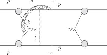
Figure 9. An example of diagrams with Glauber couplings between non-Glauber couplings and the final cut, where the dot lines represent Glauber gluons and the circle lines represent collinear gluons. |
For general diagrams, one may consider the flow of the plus momenta of plus-collinear particles. According to the discussions in section 6.1 , the plus momenta should flow from these collinear particles to the hard vertex or the final cut. We consider the couplings involving these collinear particles through the order of the flow26(According to the physical picture in [6, 34], such order should be definite on pinch singular surfaces.). We can define the momenta of these particles so that the plus momenta of these particles are positive. We then integrate out the minus momenta of these collinear particles by taking the residues of poles of the vertex from which the plus momenta of the collinear particles flow out of. If we meet Glauber couplings before non-Glauber couplings in some diagrams then there are some Glauber gluons of which all poles of the minus momenta (no less than two) locate in the upper half plane as shown in the example figure 9 and the formula (112 )27(These poles originate from the propagators of plus collinear particles coupling to Glauber gluons and vertexes which plus momenta of these particles flow into.). Hence these diagrams vanish after the cancellation of interactions with the coordinates $\widetilde{{n}_{+}}\cdot x$ greater than that of the hard collision.
For Glauber couplings of minus-collinear and soft particles, one may consider the flow of the minus momenta of these particles. According to the discussions in section 6.2 , we can consider these couplings through the order of the flow and meet the hard vertex or the final cut finally. We define the momenta of these particles so that the minus momenta of these particles are positive. Be similar to the Glauber couplings of plus-collinear particles, if we meet Glauber couplings before non-Glauber couplings in some diagrams then all poles of the plus momenta(no less than two) of some Glauber gluons locate in the upper half plane. These diagrams do not contribute to ${ \mathcal H }(P,\bar{P},{q}^{+},{q}^{-})$.
In summary, the active-spectator coherence with the coordinates $\widetilde{{n}_{+}}\cdot x$ greater than those of Glauber interactions cancel out in ${ \mathcal H }(P,\bar{P},{q}^{+},{q}^{-})$. As a result, the summation over final states in ${ \mathcal H }(P,\bar{P},{q}^{+},{q}^{-})$ is inclusive enough for spectator–spectator and spectator-soft Glauber interactions involving A+G even if there are detected final states. This is crucial in the cancellation of these Glauber interactions.
6.4. Cancellation of spectator–spectator and spectator-soft Glauber subgraphs
After excluding the effects of the active-spectator coherence, the Glauber subgraphs involving A+G factorize from other parts of ${ \mathcal H }(P,\bar{P},{q}^{+},{q}^{-})$. We can then consider the subgraphs separately.
An example of cancellation of spectator-soft and spectator–spectator Glauber exchange involving A+G is shown in figure 10.
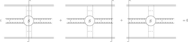
Figure 10. An example of cancellation of spectator-spectator and spectator-soft Glauber subgraphs. |
To confirm the cancellation of spectator–spectator and spectator-soft Glauber gluons no matter the initial spectators of the Glauber subprocess are on-shell or not, let us first consider an example shown in figure 11.
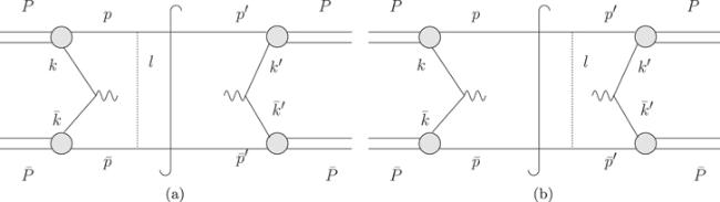
Figure 11. An example of the summation over spectator-spectator elastic scatterings. |
We have
$\begin{eqnarray}\begin{array}{l}{\rm{Figure}}\,11=\displaystyle \int \displaystyle \frac{{\rm{d}}{l}^{+}}{2\pi }\displaystyle \int \displaystyle \frac{{\rm{d}}{l}^{-}}{2\pi }\displaystyle \int \displaystyle \frac{{\rm{d}}{p}^{-}}{2\pi }\displaystyle \int \displaystyle \frac{{\rm{d}}{\bar{p}}^{+}}{2\pi }\displaystyle \int \displaystyle \frac{{\rm{d}}{p}^{{\prime} -}}{2\pi }\displaystyle \int \displaystyle \frac{{\rm{d}}{\bar{p}}^{{\prime} +}}{2\pi }\\ \quad \times \displaystyle \frac{{\rm{i}}}{{P}^{-}-{k}^{-}-{p}^{-}+{\rm{i}}\varepsilon }\displaystyle \frac{{\rm{i}}}{{\bar{P}}^{+}-{\bar{k}}^{+}-{\bar{p}}^{+}+{\rm{i}}\varepsilon }\\ \quad \times \left(\displaystyle \frac{{\rm{i}}\delta \left({p}^{{\prime} -}\,+\,\tfrac{{\left({p}_{\perp }^{{\prime} }\right)}^{2}}{2{p}^{{\prime} +}}\right)}{{p}^{-}\,+\,\tfrac{{\left({p}_{\perp }\right)}^{2}}{2{p}^{+}}+{\rm{i}}\varepsilon }\displaystyle \frac{{\rm{i}}\delta \left({\bar{p}}^{{\prime} +}\,+\,\tfrac{{\left({\bar{p}}_{\perp }^{{\prime} }\right)}^{2}}{2{\bar{p}}^{{\prime} -}}\right)}{{\bar{p}}^{+}\,+\,\tfrac{{\left({\bar{p}}_{\perp }\right)}^{2}}{2{\bar{p}}^{-}}+{\rm{i}}\varepsilon }\displaystyle \frac{{\rm{i}}}{{p}^{-}-{l}^{-}-{p}^{{\prime} -}+{\rm{i}}\varepsilon }\right.\\ \quad \times \displaystyle \frac{{\rm{i}}}{{\bar{p}}^{+}+{l}^{+}-{\bar{p}}^{{\prime} +}+{\rm{i}}\varepsilon }\displaystyle \frac{-{\rm{i}}}{{l}_{\perp }^{2}}+\displaystyle \frac{{\rm{i}}}{{l}_{\perp }^{2}}\displaystyle \frac{-{\rm{i}}}{{\bar{p}}^{{\prime} +}-{\bar{p}}^{+}-{l}^{+}-{\rm{i}}\varepsilon }\\ \left.\displaystyle \frac{-{\rm{i}}}{{p}^{{\prime} -}+{l}^{-}-{p}^{-}-{\rm{i}}\varepsilon }\displaystyle \frac{-{\rm{i}}\delta \left({\bar{p}}^{+}\,+\,\tfrac{{\left({\bar{p}}_{\perp }\right)}^{2}}{2{\bar{p}}^{-}}\right)}{{\bar{p}}^{{\prime} +}\,+\,\tfrac{{\left({\bar{p}}_{\perp }^{{\prime} }\right)}^{2}}{2{\bar{p}}^{{\prime} -}}-{\rm{i}}\varepsilon }\displaystyle \frac{-{\rm{i}}\delta \left({p}^{-}\,+\,\tfrac{{\left({p}_{\perp }\right)}^{2}}{2{p}^{+}}\right)}{{p}^{{\prime} -}\,+\,\tfrac{{\left({p}_{\perp }^{{\prime} }\right)}^{2}}{2{p}^{{\prime} +}}+{\rm{i}}\varepsilon }\right)\\ \quad \times \displaystyle \frac{-{\rm{i}}}{{P}^{-}-{k}^{{\prime} -}-{p}^{{\prime} -}-{\rm{i}}\varepsilon }\displaystyle \frac{-{\rm{i}}}{{\bar{P}}^{+}-{\bar{k}}^{{\prime} +}-{\bar{p}}^{{\prime} +}-{\rm{i}}\varepsilon }\\ \quad \times ({\rm{terms}}\,{\rm{independent}}\,{\rm{of}}\,{p}^{-}\,{\rm{and}}\,{p}^{{\prime} -}\,{\rm{and}}\,{l}^{-}\,{\rm{and}}\,{\bar{p}}^{+}\,\\ \quad {\rm{and}}\,{\bar{p}}^{{\prime} +}\,{\rm{and}}\,{l}^{+}),\end{array}\end{eqnarray}$
where the iϵ term in the propagator of l has been dropped as Glauber gluons are off-shell. After integrating out l+ and l−, we have
$\begin{eqnarray}\begin{array}{l}{\rm{Figure}}\,11=\displaystyle \int \displaystyle \frac{{\rm{d}}{p}^{-}}{2\pi }\displaystyle \int \displaystyle \frac{{\rm{d}}{\bar{p}}^{+}}{2\pi }\displaystyle \int \displaystyle \frac{{\rm{d}}{p}^{{\prime} -}}{2\pi }\displaystyle \int \displaystyle \frac{{\rm{d}}{\bar{p}}^{{\prime} +}}{2\pi }\\ \quad \times \displaystyle \frac{{\rm{i}}}{{P}^{-}-{k}^{-}-{p}^{-}+{\rm{i}}\varepsilon }\displaystyle \frac{{\rm{i}}}{{\bar{P}}^{+}-{\bar{k}}^{+}-{\bar{p}}^{+}+{\rm{i}}\varepsilon }\\ \quad \times \left(\displaystyle \frac{{\rm{i}}\delta \left({p}^{{\prime} -}\,+\,\tfrac{{\left({p}_{\perp }^{{\prime} }\right)}^{2}}{2{p}^{{\prime} +}}\right)}{{p}^{-}\,+\,\tfrac{{\left({p}_{\perp }\right)}^{2}}{2{p}^{+}}+{\rm{i}}\varepsilon }\displaystyle \frac{{\rm{i}}\delta \left({\bar{p}}^{{\prime} +}\,+\,\tfrac{{\left({\bar{p}}_{\perp }^{{\prime} }\right)}^{2}}{2{\bar{p}}^{{\prime} -}}\right)}{{\bar{p}}^{+}\,+\,\tfrac{{\left({\bar{p}}_{\perp }\right)}^{2}}{2{\bar{p}}^{-}}+{\rm{i}}\varepsilon }\displaystyle \frac{-{\rm{i}}}{{l}_{\perp }^{2}}\right.\\ \quad \left.+\displaystyle \frac{{\rm{i}}}{{l}_{\perp }^{2}}\displaystyle \frac{-{\rm{i}}\delta \left({\bar{p}}^{+}\,+\,\tfrac{{\left({\bar{p}}_{\perp }\right)}^{2}}{2{\bar{p}}^{-}}\right)}{{\bar{p}}^{{\prime} +}\,+\,\tfrac{{\left({\bar{p}}_{\perp }^{{\prime} }\right)}^{2}}{2{\bar{p}}^{{\prime} -}}-{\rm{i}}\varepsilon }\displaystyle \frac{-{\rm{i}}\delta \left({p}^{-}\,+\,\tfrac{{\left({p}_{\perp }\right)}^{2}}{2{p}^{+}}\right)}{{p}^{{\prime} -}\,+\,\tfrac{{\left({p}_{\perp }^{{\prime} }\right)}^{2}}{2{p}^{{\prime} +}}+{\rm{i}}\varepsilon }\right)\\ \quad \times \displaystyle \frac{-{\rm{i}}}{{P}^{-}-{k}^{{\prime} -}-{p}^{{\prime} -}-{\rm{i}}\varepsilon }\displaystyle \frac{-{\rm{i}}}{{\bar{P}}^{+}-{\bar{k}}^{{\prime} +}-{\bar{p}}^{{\prime} +}-{\rm{i}}\varepsilon }\\ \quad \times ({\rm{terms}}\,{\rm{independent}}\,{\rm{of}}\,{p}^{-}\,{\rm{and}}\,{p}^{{\prime} -}\,{\rm{and}}\,{\bar{p}}^{+}\,{\rm{and}}\,{\bar{p}}^{{\prime} +}).\end{array}\end{eqnarray}$
We then integrate out p− and ${p}^{{\prime} -}$ and ${\bar{p}}^{+}$ and ${\bar{p}}^{{\prime} +}$ and have
$\begin{eqnarray}{\rm{Figure}}\,11=0.\end{eqnarray}$
That is, the Glauber exchanges cancel out in figure 11 no matter whether the initial spectators are on-shell or not.
For general cases, one may consider Glauber couplings according to the $\widetilde{{n}_{+}}\cdot x$-order. We take the substitution (95 ) in couplings involving plus-collinear particles. After the substitution, the minus momenta of plus collinear particles are independent of each other. We then integrate out the minus momenta of Glauber gluons coupling to plus-collinear particles by taking residues of the Glauber vertexes. These vertexes look like
$\begin{eqnarray}\displaystyle \frac{-{\rm{i}}}{{l}_{i}\cdots +\,{\rm{i}}\varepsilon }.\end{eqnarray}$
After these integrals, the Glauber exchange subprocess relies on the minus momenta of initial plus-collinear spectators only through their propagators or wave function. In other words, the whole process (including the Glauber and non-Glauber subprocess) relies on the minus momenta of the spectators only through the vertex at which the spectators are produced and propagators or wave functions of the spectators.28(For example, one may check the p−-terms in (115 ).) We then integrate out the minus momenta of the spectators by taking the poles of the propagators (if the spectators are off-shell) or using the on-shell condition(if the spectators are on-shell). Obviously, these two results are equivalent to each other. For Glauber couplings of other particles, we have similar results. That is, the cancellation of spectator–spectator and spectator-soft Glauber gluons is irrelevant to the off-shellness of initial particles of the Glauber subprocess at the leading power of λ and η.
Generally, one may consider the $\widetilde{{n}_{+}}\cdot x$-evolution of spectators and soft particles. Such evolution is unitary as ${\widetilde{{n}_{+}}}^{\mu }$ is time-like. As a result, one has a $\widetilde{{n}_{+}}\cdot x$ version of the optical theorem
$\begin{eqnarray}{T}_{+}^{\dagger }{T}_{+}=-{\rm{i}}({T}_{+}-{T}_{+}^{\dagger }),\end{eqnarray}$
where T+ represents the $\widetilde{{n}_{+}}\cdot x$-version of the scattering matrix. According to the relation (118 ), Glauber exchange with the coordinates $\widetilde{{n}_{+}}\cdot x$ greater than those of the active-spectator coherence cancels out at the leading order of λ. The optical theorem (118 ) is the direct result of the unitarity of the $\widetilde{{n}_{+}}\cdot x$-evolution operator U+G( ∞ , − ∞ ) in (85 ). The cancellation in figure 10 is a special case of (118 ). That is
$\begin{eqnarray}\begin{array}{l}{U}_{+G}(\infty ,-\infty ){U}_{+G}(\infty ,-\infty )=1\\ \quad \Rightarrow {T}_{+}^{\dagger }{T}_{+}=-{\rm{i}}({T}_{+}-{T}_{+}^{\dagger }).\end{array}\end{eqnarray}$
Hence the graphic cancellation of spectator–spectator and spectator-soft Glauber exchange involving A+G based on the relation (118 ) is equivalent to our operator level method in section 5.3 .
After the cancellation of the Glauber gluons A+G, one may consider an effective theory free from A+G. Calculations of ${ \mathcal H }(P,\bar{P},{q}^{+},{q}^{-})$ in this effective theory are equivalent to those in the theory (7 ). One can then consider the $\widetilde{{n}_{-}}\cdot x$-evolution and repeat the procedure of A+G to see the cancellation of A−G. The cancellation originates from the $\widetilde{{n}_{-}}\cdot x$ version of the optical theorem, which is equivalent to our operator level method.
7. Conclusions and discussions
We discuss the Glauber gluon effects in hadron collisions in this paper. It is proved that final state interactions cancel out in processes inclusive enough. For a time-like evolution(like $\widetilde{{n}_{+}}\cdot x$-evolution in section 5.1 ) which is approximately equivalent to a light-like evolution, we have a similar result. That is, interactions with the coordinates $\widetilde{n}\cdot x$ greater than that of the hard collision cancel out in processes inclusive enough. After the cancellation, the active-spectator coherence no longer disturbs us and we prove the cancellation of the spectator-spectator and spectator-soft Glauber exchanges for processes inclusive enough. We also present the proof of eikonalization of active-spectator and active-active and active-soft type Glauber exchanges. According to our discussions, these Glauber gluons should be viewed as zero-bins of collinear or soft gluons and absorbed into directions of collinear and soft Wilson lines of the hard vertex. The graphic cancellation of the spectator-spectator and spectator-soft Glauber exchanges are also discussed here to show how such graphic cancellation is related to operator level skills in this paper.
Exactly, the cancellation of interactions with the coordinates $\widetilde{{n}_{+}}\cdot x$ greater than that of the hard collision is equivalent to the cancellation of final states interactions as $\widetilde{{n}_{+}}$ is time-like. On the other hand, $\widetilde{{n}_{+}}$ is approximately light-like and the $\widetilde{{n}_{+}}\cdot x$-evolution of collinear and soft particles is approximately equivalent to the light cone evolution of these particles at the mass center frame of initial hadrons as discussed in sections 6.1 and 6.2 . This explains why proofs based on the time-like evolution here give the same conclusion as those based on the light cone evolution [4].
According to our discussions, the eikonal approximation is crucial in the definition of collinear and soft modes at loop level. At the tree level, collinear and soft modes are characterized by their momenta. Considering that one usually runs over all momenta regions in practical loop integrals, the subtraction scheme to avoid double counting in loop level definition of different modes is necessary for the definition. Although the details of such a subtraction scheme are not concerned here, higher order definitions of different modes depending on the manner in which they couple to lower order modes. Especially, the eikonalized parts of couplings between collinear and other modes should be absorbed into collinear-collinear or soft-collinear or ultrasoft-collinear couplings. According to these definitions, active-spectator and active-soft exchanged gluons should be absorbed into the definition of loop level collinear and soft gluons.
Spectator-active interactions with the coordinates $\widetilde{{n}_{+}}\cdot x$($\widetilde{{n}_{-}}\cdot x$) greater than those of Glauber exchanges should be treated carefully as they may obstruct the summation of spectator-soft and spectator-spectator Glauber exchanges. Fortunately, these interactions cancel out for processes considered here as discussed in section 5.2 . Intuitively, spectator-soft and spectator-spectator exchange of Glauber gluons A+G and A−G should occur at the vertexes with the coordinates x+ and x− equivalent to those of the hard collision according to the classical trajectories of collinear particles29(Pinch singular surfaces are related to classical trajectories as discussed in [34].) and locality of the Glauber propagators in the x+ and x− directions. Therefore one should not be surprised to see such a cancellation.
Considering that Glauber couplings may change the transverse momenta of final particles, the summation over these final states, especially the integration over transverse momenta of these final states, is necessary for the cancellation of Glauber exchanges. While considered observable is not inclusive enough, the final states may not form the invariant subspace of the evolution induced by Glauber couplings and the Glauber cancellations induced by the unitarity of the evolution may break up. That is to say, our proofs of Glauber cancellation only work for quantities inclusive enough. For electromagnetic processes like the Drell–Yan process, the result is stronger. In these processes, there are no QCD interactions between the lepton pair l+l− and undetected states X. Thus QCD interactions between final states do not change the total momentum of the lepton pair at the lowest order of electromagnetic interactions. Hence the final state interactions cancel out in these processes even if q⊥ is not integrated out.
According to our discussions, the operator level factorization theorem should be tightly related to the graphic aspects of the theorem. However, the operator level factorization differs from the graphic factorization through the aspects: (1) instead of explicit perturbative calculations, we get the operator level cancellation of final state interactions through the unitarity of the time evolution operator; (2) instead of light cone perturbative series, we exclude the active-spectator coherence with x+ and x− greater than those of spectator–spectator and spectator-soft Glauber exchanges through the (operator level) evolution property of collinear particles; (3) instead of light cone perturbative series, we get the cancellation of spectator-spectator and spectator-soft Glauber exchanges through the operator level unitarity.
Acknowledgments
The work of G L Zhou is supported by The National Nature Science Foundation of China under Grant No. 11805151 and The Scientific Research Foundation for the Doctoral Program of Xi’an University of Science and Technology under Grant No. 6310116055 and The Scientific Fostering Foundation of Xi’an University of Science and Technology under Grant No. 201709. The work of Z X Yan is supported by The Department of Shanxi Province Natural Science Foundation of China under Grant No. 2015JM1027. The work of F Li is supported by China Postdoctoral Foundation under Grant No. 2015M581824, 20161001 and International Postdoctoral Exchange Fellowship Program between JUELICH and OCPC.
Appendix A. Time evolution operator of the effective theory
We discuss the time evolution operator of the effective theory here. Generally speaking, the time evolution operator in the interaction picture reads7 ), which should be viewed as constraints. According to the effective action (7 ), one has
$\begin{eqnarray}U({t}_{1},{t}_{2})={{\rm{e}}}^{{\rm{i}}{H}_{0}{t}_{2}}{{\rm{e}}}^{-{\rm{i}}H({t}_{2}-{t}_{1})}{{\rm{e}}}^{-{\rm{i}}{H}_{0}{t}_{1}},\end{eqnarray}$
where H0 and H are the free and full Hamiltonian of the theory. However, the Hamiltonian formulation of non-Abelian gauge theory is quite nontrivial (see e.g. [35, 36]), not to mention the difficulties caused by Glauber gluon fields in ( $\begin{eqnarray}\begin{array}{l}{\left({{ \mathcal P }}_{\perp }\right)}^{2}n\cdot {A}_{{nG}}^{a}\\ \quad =g({\bar{\xi }}_{\bar{n}}{t}^{a}{/}\!\!\!\!{n}{\xi }_{\bar{n}})+2{g}{\rm{tr}}\{{\bar{c}}_{\bar{n}}[{\rm{i}}n\cdot {{ \mathcal D }}_{\bar{n}},[{t}^{a},{c}_{\bar{n}}]]\}\\ \quad +\displaystyle \frac{2}{g}{\rm{tr}}\{[{\rm{i}}{{ \mathcal D }}_{\bar{n}}^{\mu }+{{gA}}_{\bar{n}}^{\mu },{\rm{i}}n\cdot {{ \mathcal D }}_{\bar{n}}+{gn}\cdot {A}_{\bar{n}}][{\rm{i}}{{ \mathcal D }}_{\bar{n}\mu }\\ \quad +{{gA}}_{\bar{n}\mu },{t}^{a}]\}\\ \quad +g({\bar{\psi }}_{s}{t}^{a}{/}\!\!\!\!{n}{\psi }_{s})+2{g}{\rm{tr}}\{{\bar{c}}_{s}[n\cdot { \mathcal P },[{t}^{a},{c}_{s}]]\}\\ \quad +\displaystyle \frac{2}{g}{\rm{tr}}\{[{{ \mathcal P }}^{\mu }+{{gA}}_{s}^{\mu }+g\sum _{{n}^{{\prime} }\ne n}\bar{{n}^{{\prime} }}\cdot {A}_{{n}^{{\prime} }G}{n}^{{\prime} \mu },n\cdot { \mathcal P }\\ \quad +{gn}\cdot {A}_{s}+g\sum _{{n}^{{\prime} }\ne n}\bar{{n}^{{\prime} }}\cdot {A}_{{n}^{{\prime} }G}n\cdot {n}^{{\prime} }]\\ \quad \times [{{ \mathcal P }}_{\mu }+{{gA}}_{s\mu }+g\sum _{{n}^{{\prime} }\ne n}\bar{{n}^{{\prime} }}\cdot {A}_{{n}^{{\prime} }G}{n}_{{\prime} \mu },{t}^{a}]\}\\ \quad \times {\left({{ \mathcal P }}_{\perp }\right)}^{2}\bar{n}\cdot {A}_{{nG}}^{a}\\ \quad =g({\bar{\xi }}_{n}{t}^{a}{/}\!\!\!\!{n}{\xi }_{n})+2{g}{\rm{tr}}\{{\bar{c}}_{n}[{\rm{i}}\bar{n}\cdot {{ \mathcal D }}_{n},[{t}^{a},{c}_{n}]]\}\\ \quad +\displaystyle \frac{2}{g}{\rm{tr}}\{[{\rm{i}}{{ \mathcal D }}_{n}^{\mu }+{{gA}}_{n}^{\mu },{\rm{i}}\bar{n}\cdot {{ \mathcal D }}_{n}+g\bar{n}\cdot {A}_{n}]\\ \quad \times [{\rm{i}}{{ \mathcal D }}_{n\mu }+{{gA}}_{n\mu },{t}^{a}]\},\end{array}\end{eqnarray}$
where collinear and soft momenta are not displayed explicitly for simplicity.Solving the constraints corresponding to Glauber gluon fields is equivalent to integrating out Glauber gluon fields in the effective theory. Let us consider the solution of n · An,G
$\begin{eqnarray}\begin{array}{l}n\cdot {A}_{{nG}}^{a}\\ \quad =\displaystyle \frac{g}{{\left({{ \mathcal P }}_{\perp }\right)}^{2}}({\bar{\xi }}_{\bar{n}}{t}^{a}{/}\!\!\!\!{n}{\xi }_{\bar{n}})+\displaystyle \frac{2g}{{\left({{ \mathcal P }}_{\perp }\right)}^{2}}{\rm{tr}}\{{\bar{c}}_{\bar{n}}[{\rm{i}}n\cdot {{ \mathcal D }}_{\bar{n}},[{t}^{a},{c}_{\bar{n}}]]\}\\ \quad +\displaystyle \frac{1}{{\left({{ \mathcal P }}_{\perp }\right)}^{2}}\displaystyle \frac{2}{g}{\rm{tr}}\{[{\rm{i}}{{ \mathcal D }}_{\bar{n}}^{\mu }+{{gA}}_{\bar{n}}^{\mu },{\rm{i}}n\cdot {{ \mathcal D }}_{\bar{n}}+{gn}\cdot {A}_{\bar{n}}]\\ \quad \times [{\rm{i}}{{ \mathcal D }}_{\bar{n}\mu }+{{gA}}_{\bar{n}\mu },{t}^{a}]\}\\ \quad +\displaystyle \frac{g}{{\left({{ \mathcal P }}_{\perp }\right)}^{2}}({\bar{\psi }}_{s}{t}^{a}{/}\!\!\!\!{n}{\psi }_{s})+\displaystyle \frac{2g}{{\left({{ \mathcal P }}_{\perp }\right)}^{2}}{\rm{tr}}\{{\bar{c}}_{s}[n\cdot { \mathcal P },[{t}^{a},{c}_{s}]]\}\\ \quad +\displaystyle \frac{1}{{\left({{ \mathcal P }}_{\perp }\right)}^{2}}\displaystyle \frac{2}{g}{\rm{tr}}\{[{{ \mathcal P }}^{\mu }+{{gA}}_{s}^{\mu }+g\sum _{{n}^{{\prime} }\ne n}\bar{{n}^{{\prime} }}\cdot {A}_{{n}^{{\prime} }G}{n}^{{\prime} \mu },n\cdot { \mathcal P }\\ \quad +{gn}\cdot {A}_{s}+g\sum _{{n}^{{\prime} }\ne n}\bar{{n}^{{\prime} }}\cdot {A}_{{n}^{{\prime} }G}n\cdot {n}^{{\prime} }]\\ \quad \times [{{ \mathcal P }}_{\mu }+{{gA}}_{s\mu }+g\sum _{{n}^{{\prime} }\ne n}\bar{{n}^{{\prime} }}\cdot {A}_{{n}^{{\prime} }G}{n}_{{\prime} \mu },{t}^{a}]\}.\end{array}\end{eqnarray}$
We substitute the solution into couplings between n-collinear quarks and the Glauber gluons An,G and have
$\begin{eqnarray}\begin{array}{l}g{\bar{\xi }}_{n}n\cdot {A}_{{nG}}{/}\!\!\!\!{\bar{n}}{\xi }_{n}\\ \quad ={\bar{\xi }}_{n}{t}^{a}{/}\!\!\!\!{\bar{n}}{\xi }_{n}\displaystyle \frac{{g}^{2}}{{\left({{ \mathcal P }}_{\perp }\right)}^{2}}{\bar{\xi }}_{\bar{n}}{t}^{a}{/}\!\!\!\!{n}{\xi }_{\bar{n}}+{\bar{\xi }}_{n}{t}^{a}{/}\!\!\!\!{\bar{n}}{\xi }_{n}\\ \quad \times \displaystyle \frac{2{g}^{2}}{{\left({{ \mathcal P }}_{\perp }\right)}^{2}}{\rm{tr}}\{{\bar{c}}_{\bar{n}}[{\rm{i}}n\cdot {{ \mathcal D }}_{\bar{n}},[{t}^{a},{c}_{\bar{n}}]]\}\\ \quad +{\bar{\xi }}_{n}{t}^{a}{/}\!\!\!\!{\bar{n}}{\xi }_{n}\displaystyle \frac{2}{{\left({{ \mathcal P }}_{\perp }\right)}^{2}}{\rm{tr}}\{[{\rm{i}}{{ \mathcal D }}_{\bar{n}}^{\mu }+{{gA}}_{\bar{n}}^{\mu },{\rm{i}}n\cdot {{ \mathcal D }}_{\bar{n}}\\ \quad +{gn}\cdot {A}_{\bar{n}}][{\rm{i}}{{ \mathcal D }}_{\bar{n}\mu }+{{gA}}_{\bar{n}\mu },{t}^{a}]\}\\ \quad +{\bar{\xi }}_{n}{t}^{a}{/}\!\!\!\!{\bar{n}}{\xi }_{n}\displaystyle \frac{{g}^{2}}{{\left({{ \mathcal P }}_{\perp }\right)}^{2}}({\bar{\psi }}_{s}{t}^{a}{/}\!\!\!\!{n}{\psi }_{s})+{\bar{\xi }}_{n}{t}^{a}{/}\!\!\!\!{\bar{n}}{\xi }_{n}\\ \quad \times \displaystyle \frac{2{g}^{2}}{{\left({{ \mathcal P }}_{\perp }\right)}^{2}}{\rm{tr}}\{{\bar{c}}_{s}[n\cdot { \mathcal P },[{t}^{a},{c}_{s}]]\}\\ \quad +{\bar{\xi }}_{n}{t}^{a}{/}\!\!\!\!{\bar{n}}{\xi }_{n}\displaystyle \frac{2}{{\left({{ \mathcal P }}_{\perp }\right)}^{2}}{\rm{tr}}\{[{{ \mathcal P }}^{\mu }+{{gA}}_{s}^{\mu }\\ \quad +g\sum _{{n}^{{\prime} }\ne n}\bar{{n}^{{\prime} }}\cdot {A}_{{n}^{{\prime} }G}{n}^{{\prime} \mu },n\cdot { \mathcal P }\\ \quad +{gn}\cdot {A}_{s}+g\sum _{{n}^{{\prime} }\ne n}\bar{{n}^{{\prime} }}\cdot {A}_{{n}^{{\prime} }G}n\cdot {n}^{{\prime} }]\\ \quad \times [{{ \mathcal P }}_{\mu }+{{gA}}_{s\mu }+g\sum _{{n}^{{\prime} }\ne n}\bar{{n}^{{\prime} }}\cdot {A}_{{n}^{{\prime} }G}{n}_{{\prime} \mu },{t}^{a}]\}.\end{array}\end{eqnarray}$
While neglecting the Glauber gluon terms in the solution of n · AnG, we obtain the scattering processes induced by the exchange of a Glauber gluon. Some examples of these scattering processes are shown in figure A1
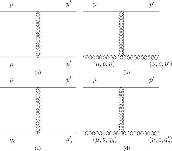
Figure A1. Examples of tree level elastics scattering processes induced by a Glauber exchange. Figure (a) shows the scattering between n-collinear and $\bar{n}$-collinear quarks. Figure (b) shows the scattering between n-collinear quarks and transverse polarized $\bar{n}$-collinear gluons. Figure (c) shows the scattering between n-collinear and soft quarks. Figure (d) shows the scattering between n-collinear quarks and soft gluons. |
At leading of power λ, figure A1 reads
$\begin{eqnarray}\begin{array}{rcl}\mathrm{Figure}\,{\rm{A}}1(a) & = & -\frac{{\rm{i}}{g}^{2}}{(\vec{{p}^{^{\prime} }}-\vec{p}{)}_{\perp }^{2}}\bar{u}({p}^{^{\prime} }){t}^{a}{/}\!\!\!\!{\bar{n}}u(p)\bar{u}({\bar{p}}^{^{\prime} }){t}^{a}{/}\!\!\!\!{n}u(\bar{p})\\ \mathrm{Figure}\,{\rm{A}}1(b) & = & -\frac{2{g}^{2}{f}^{{abc}}}{(\vec{{p}^{^{\prime} }}-\vec{p}{)}_{\perp }^{2}}\bar{u}({p}^{^{\prime} }){t}^{a}{/}\!\!\!\!{\bar{n}}u(p){g}_{\perp }^{\mu \nu }n\cdot \bar{p}\\ \mathrm{Figure}\,{\rm{A}}1(c) & = & -\frac{{\rm{i}}{g}^{2}}{(\vec{{q}_{s}^{\mbox{'}}}-\vec{{q}_{s}}{)}_{\perp }^{2}}\bar{u}({p}^{^{\prime} }){t}^{a}{/}\!\!\!\!{\bar{n}}u(p)\bar{u}({q}_{s}){t}^{a}{/}\!\!\!\!{n}u({q}_{s})\\ \mathrm{Figure}\,{\rm{A}}1(d) & = & -\frac{{g}^{2}{f}^{{abc}}}{(\vec{{q}_{s}^{\mbox{'}}}-\vec{{q}_{s}}{)}_{\perp }^{2}}\bar{u}({p}^{^{\prime} }){t}^{a}{/}\!\!\!\!{\bar{n}}u(p)({n}^{\mu }({q}_{s}^{\mbox{'}\nu }-2{q}_{s}^{\nu })\\ & & +{n}^{\nu }({q}_{s}^{\mu }-2{q}_{s}^{\mbox{'}\mu })+2n\cdot {q}_{s}{g}^{\mu \nu }).\end{array}\end{eqnarray}$
For the Glauber gluon terms in equation (A4 ), one may obtain their contribution order by order and see elastic processes induced by the exchange of more sequential Glauber gluons. We show some examples of such elastic scattering in figure A2.

Figure A2. Examples of tree level elastics scattering processes induced by two sequential Glauber gluons, where qs and ${q}_{s}^{{\prime} }$ represent soft gluons. |
At leading of power λ, figure A2 readsA5 ) and (A6 ) are equivalent to the full QCD results at the leading power of λ.
$\begin{eqnarray}\begin{array}{l}\mathrm{Figure}\,{\rm{A}}2(a)=\frac{{g}^{3}{f}^{{abc}}}{(\vec{{p}^{^{\prime} }}-\vec{p}{)}_{\perp }^{2}(\vec{{\bar{p}}^{^{\prime} }}-\vec{\bar{p}}{)}_{\perp }^{2}}\\ \quad \times \bar{u}({p}^{{\prime} }){t}^{a}{/}\!\!\!\!{\bar{n}}u(p)\bar{u}({\bar{p}}^{{\prime} }){t}^{b}{/}\!\!\!\!{n}u(\bar{p})\\ \quad \times \left({p}^{^{\prime} }-p-{\bar{p}}^{^{\prime} }+\bar{p}{)}_{\perp }^{\mu }\right.\\ \quad \left.+2n\cdot ({\bar{p}}^{^{\prime} }-\bar{p})-2\bar{n}\cdot ({p}^{^{\prime} }-p\right)\\ \mathrm{Figure}\,{\rm{A}}2(b)=-\frac{{\rm{i}}{g}^{4}}{(\vec{{p}^{^{\prime} }}-\vec{p}{)}_{\perp }^{2}(\vec{{\bar{p}}^{^{\prime} }}-\vec{\bar{p}}{)}_{\perp }^{2}}\\ \quad \times \bar{u}({p}^{{\prime} }){t}^{a}{/}\!\!\!\!{\bar{n}}u(p)\bar{u}({\bar{p}}^{{\prime} }){t}^{b}{/}\!\!\!\!{n}u(\bar{p})\\ \quad \times \left({f}^{{abe}}{f}^{{cde}}({\bar{n}}^{\mu }{n}^{\nu }-{n}^{\mu }{\bar{n}}^{\nu })+{f}^{{ace}}{f}^{{bde}}({g}^{\mu \nu }-{n}^{\mu }{\bar{n}}^{\nu })\right.\\ \quad \left.+{f}^{{ade}}{f}^{{bce}}({g}^{\mu \nu }-{\bar{n}}^{\mu }{n}^{\nu }\right).\end{array}\end{eqnarray}$
One can verify that equations (For couplings between Glauber and n-collinear gluons, we have similar results. Although Glauber gluons are not integrated out here, one should keep in mind that they are constraints and do not correspond to any quantum states.
Instead of the Hamiltonian formula, we would like to discuss the time evolution operator in the frame of the path integral. Let us start from the time evolution operator of an ordinary gauge theory. According to the relation between the Hamiltonian formulation and path integral method, one hasA7 ) can be extended to arbitrary states(including non-physical states)30(According to the discussions in [37], physical states should be annihilated by the BRST-charge.)
$\begin{eqnarray}\begin{array}{l}\left\langle {B}_{{\rm{phy}}}| U({t}_{2},{t}_{1})| {A}_{{\rm{phy}}}\right\rangle \\ \quad \equiv \left\langle {B}_{{\rm{phy}}}| {{\rm{e}}}^{{\rm{i}}{H}_{0}{t}_{2}}{{\rm{e}}}^{-{\rm{i}}H({t}_{2}-{t}_{1})}{{\rm{e}}}^{-{\rm{i}}{H}_{0}{t}_{1}}| {A}_{{\rm{phy}}}\right\rangle \\ \quad ={ \mathcal C }\displaystyle \int [D{\psi }_{2}][D{\bar{\psi }}_{2}][{{DA}}_{2}^{\mu }][{{Dc}}_{2}][D{\bar{c}}_{2}]\\ \quad \times \displaystyle \int [D\psi ][D\bar{\psi }][{{DA}}^{\mu }][{Dc}][D\bar{c}]\\ \quad \times \displaystyle \int [D{\psi }_{1}][D{\bar{\psi }}_{1}][{{DA}}_{1}^{\mu }][{{Dc}}_{1}][D{\bar{c}}_{1}]\left\langle {B}_{{\rm{phy}}}| {\psi }_{2},{\bar{\psi }}_{2},{A}_{2}^{\mu }\right\rangle \\ \quad \times \left\langle {\psi }_{1},{\bar{\psi }}_{1},{A}_{1}^{\mu }| {A}_{{\rm{phy}}}\right\rangle \\ \quad \times \,\exp (-{\rm{i}}{I}_{0}({\psi }_{2},{\bar{\psi }}_{2},{A}_{2}^{\mu },{c}_{2},{\bar{c}}_{2})({t}_{2},0))\\ \quad \times \,\exp ({\rm{i}}I(\psi ,\bar{\psi },{A}^{\mu },c,\bar{c})({t}_{2},{t}_{1}))\\ \quad \times \,\exp ({\rm{i}}{I}_{0}({\psi }_{1},{\bar{\psi }}_{1},{A}_{1}^{\mu },{c}_{1},{\bar{c}}_{1})({t}_{1},0))\end{array}\end{eqnarray}$
for arbitrary physical states $\left|{A}_{{\rm{phy}}}\right\rangle $ and $\left|{B}_{{\rm{phy}}}\right\rangle $, where ${ \mathcal C }$ is a constant independent of the fields and the states $\left|{A}_{{\rm{phy}}}\right\rangle $ and $\left|{B}_{{\rm{phy}}}\right\rangle $. The matrix element ( $\begin{eqnarray}\begin{array}{l}\left\langle B\right|U({t}_{2},{t}_{1})\left|A\right\rangle \\ \quad \equiv { \mathcal C }\displaystyle \int [D{\psi }_{2}][D{\bar{\psi }}_{2}][{{DA}}_{2}^{\mu }][{{Dc}}_{2}][D{\bar{c}}_{2}]\\ \quad \times \displaystyle \int [D\psi ][D\bar{\psi }][{{DA}}^{\mu }][{Dc}][D\bar{c}]\\ \quad \times \displaystyle \int [D{\psi }_{1}][D{\bar{\psi }}_{1}][{{DA}}_{1}^{\mu }][{{Dc}}_{1}][D{\bar{c}}_{1}]\left\langle B| {\psi }_{2},{\bar{\psi }}_{2},{A}_{2}^{\mu },{c}_{2},{\bar{c}}_{2}\right\rangle \\ \quad \times \left\langle {\psi }_{1},{\bar{\psi }}_{1},{A}_{1}^{\mu },{c}_{1},{\bar{c}}_{1}| A\right\rangle \\ \quad \times \,\exp (-{\rm{i}}{I}_{0}({\psi }_{2},{\bar{\psi }}_{2},{A}_{2}^{\mu },{c}_{2},{\bar{c}}_{2})({t}_{2},0))\\ \quad \times \,\exp ({\rm{i}}I(\psi ,\bar{\psi },{A}^{\mu },c,\bar{c})({t}_{2},{t}_{1}))\\ \quad \times \,\exp ({\rm{i}}{I}_{0}({\psi }_{1},{\bar{\psi }}_{1},{A}_{1}^{\mu },{c}_{1},{\bar{c}}_{12})({t}_{1},0)).\end{array}\end{eqnarray}$
The matrix element (A8 ) can be viewed as the Lagrangian formula of the time evolution operator.
For the effective theory, one has a similar Lagrangian formula of the time evolution operator
$\begin{eqnarray}\begin{array}{l}\left\langle B| {U}_{{{SCET}}_{G}}({t}_{2},{t}_{1})| A\right\rangle \\ \quad \equiv { \mathcal C }\displaystyle \int [D{\xi }_{n}^{(2)}\cdots ][D{\bar{\xi }}_{n}^{(2)}\cdots ][{{DA}}_{n}^{(2)\mu }\cdots ]\\ \quad \times [{{Dc}}_{n}^{(2)}\cdots ][D{\bar{c}}_{n}^{(2)}\cdots ]\\ \quad \times \displaystyle \int [D{\xi }_{n}\cdots ][D{\bar{\xi }}_{n}\cdots ][{{DA}}_{n}^{\mu }\cdots ][{{Dc}}_{n}\cdots ][D{\bar{c}}_{n}\cdots ]\\ \quad \times \displaystyle \int [D{\xi }_{n}^{(1)}\cdots ][D{\bar{\xi }}_{n}^{(1)}\cdots ][{{DA}}_{n}^{(1)\mu }\cdots ]\\ \quad \times [{{Dc}}_{n}^{(1)}\cdots ][D{\bar{c}}_{n}^{(1)}\cdots ]\\ \quad \times \,\exp (-{\rm{i}}{I}_{{eff}}^{(0)}({\xi }_{n}^{(2)},{\bar{\xi }}_{n}^{(2)},{A}_{n}^{(2)\mu },{c}_{n}^{(2)},{\bar{c}}_{n}^{(2)},\ldots )({t}_{2},0))\\ \quad \times \,\exp ({\rm{i}}{I}_{{eff}}({\xi }_{n},{\bar{\xi }}_{n},{A}_{n}^{\mu },{c}_{n},{\bar{c}}_{n},\ldots )({t}_{2},{t}_{1}))\\ \quad \times \,\exp ({\rm{i}}{I}_{{eff}}^{(0)}({\xi }_{n}^{(1)},{\bar{\xi }}_{n}^{(1)},{A}_{n}^{(1)\mu },{c}_{n}^{(1)},{\bar{c}}_{n}^{(1)},\ldots )({t}_{1},0))\\ \quad \times \left\langle B| {\xi }_{n}^{(2)},{\bar{\xi }}_{n}^{(2)},{A}_{n}^{(2)\mu },{c}_{n}^{(2)},{\bar{c}}_{n}^{(2)},\cdots \right\rangle \\ \quad \times \left\langle {\xi }_{n}^{(1)},{\bar{\xi }}_{n}^{(1)},{A}_{n}^{(1)\mu },{c}_{n}^{(1)},{\bar{c}}_{n}^{(1)},\cdots | A\right\rangle ,\end{array}\end{eqnarray}$
where ${I}_{{eff}}^{(0)}$ represents the free part of the effective action (7 ). While considering hard collision processes, the relevant time evolution operator reads
$\begin{eqnarray}\begin{array}{l}\left\langle B| {U}_{{{SCET}}_{G}}^{h}({t}_{2},{t}_{1})| A\right\rangle \\ \quad \equiv { \mathcal C }\displaystyle \int [D{\xi }_{n}^{(2)}\cdots ][D{\bar{\xi }}_{n}^{(2)}\cdots ][{{DA}}_{n}^{(2)\mu }\cdots ]\\ \quad \times [{{Dc}}_{n}^{(2)}\cdots ][D{\bar{c}}_{n}^{(2)}\cdots ]\\ \quad \times \displaystyle \int [D{\xi }_{n}\cdots ][D{\bar{\xi }}_{n}\cdots ][{{DA}}_{n}^{\mu }\cdots ]\\ \quad \times [{{Dc}}_{n}\cdots ][D{\bar{c}}_{n}\cdots ]\\ \quad \times \displaystyle \int [D{\xi }_{n}^{(1)}\cdots ][D{\bar{\xi }}_{n}^{(1)}\cdots ][{{DA}}_{n}^{(1)\mu }\cdots ][{{Dc}}_{n}^{(1)}\cdots ][D{\bar{c}}_{n}^{(1)}\cdots ]\\ \quad \times \,\exp (-{\rm{i}}{I}_{{eff}}^{(0)}({\xi }_{n}^{(2)},{\bar{\xi }}_{n}^{(2)},{A}_{n}^{(2)\mu },{c}_{n}^{(2)},{\bar{c}}_{n}^{(2)},\ldots )({t}_{2},0))\\ \quad \times \,\exp ({\rm{i}}{I}_{{eff}}({\xi }_{n},{\bar{\xi }}_{n},{A}_{n}^{\mu },{c}_{n},{\bar{c}}_{n},\ldots )({t}_{2},{t}_{1}))\\ \quad \times \,\exp \left({\rm{i}}{\displaystyle \int }_{{t}_{1}}^{{t}_{2}}{\rm{d}}t\displaystyle \int {{\rm{d}}}^{3}\vec{x}{J}_{h}({S}_{n}{W}_{n}^{\dagger }{\xi }_{n},{S}_{n}{W}_{n}^{\dagger }{A}_{n}^{\mu }{W}_{n}{S}_{n}^{\dagger },{\bar{\xi }}_{n}{W}_{n}{S}_{n}^{\dagger },\ldots )\right)\\ \quad \times \,\exp ({\rm{i}}{I}_{{eff}}^{(0)}({\xi }_{n}^{(1)},{\bar{\xi }}_{n}^{(1)},{A}_{n}^{(1)\mu },{c}_{n}^{(1)},{\bar{c}}_{n}^{(1)},\ldots )({t}_{1},0))\\ \quad \times \,\left\langle B| {\xi }_{n}^{(2)},{\bar{\xi }}_{n}^{(2)},{A}_{n}^{(2)\mu },{c}_{n}^{(2)},{\bar{c}}_{n}^{(2)},\cdots \right\rangle \\ \quad \times \left\langle {\xi }_{n}^{(1)},{\bar{\xi }}_{n}^{(1)},{A}_{n}^{(1)\mu },{c}_{n}^{(1)},{\bar{c}}_{n}^{(1)},\cdots | A\right\rangle .\end{array}\end{eqnarray}$
For $\widetilde{{n}_{+}}\cdot x$-evolution, we have similar results
$\begin{eqnarray}\begin{array}{l}\left\langle B| {U}_{{{SCET}}_{G}}(\widetilde{{n}_{+}}\cdot {x}_{2},\widetilde{{n}_{+}}\cdot {x}_{1})| A\right\rangle \\ \quad \equiv { \mathcal C }\displaystyle \int [D{\xi }_{n}^{(2)}\cdots ][D{\bar{\xi }}_{n}^{(2)}\cdots ][{{DA}}_{n}^{(2)\mu }\cdots ]\\ \quad \times [{{Dc}}_{n}^{(2)}\cdots ][D{\bar{c}}_{n}^{(2)}\cdots ]\\ \quad \times \displaystyle \int [D{\xi }_{n}\cdots ][D{\bar{\xi }}_{n}\cdots ][{{DA}}_{n}^{\mu }\cdots ][{{Dc}}_{n}\cdots ][D{\bar{c}}_{n}\cdots ]\\ \quad \times \displaystyle \int [D{\xi }_{n}^{(1)}\cdots ][D{\bar{\xi }}_{n}^{(1)}\cdots ][{{DA}}_{n}^{(1)\mu }\cdots ][{{Dc}}_{n}^{(1)}\cdots ][D{\bar{c}}_{n}^{(1)}\cdots ]\\ \quad \times \,\exp (-{\rm{i}}{I}_{{eff}}^{(0)}({\xi }_{n}^{(2)},{\bar{\xi }}_{n}^{(2)},{A}_{n}^{(2)\mu },{c}_{n}^{(2)},{\bar{c}}_{n}^{(2)},\ldots )(\widetilde{{n}_{+}}\cdot {x}_{2},0)\\ \quad \times \,\exp ({\rm{i}}{I}_{{eff}}({\xi }_{n},{\bar{\xi }}_{n},{A}_{n}^{\mu },{c}_{n},{\bar{c}}_{n},\ldots )(\widetilde{{n}_{+}}\cdot {x}_{2},\widetilde{{n}_{+}}\cdot {x}_{1})\\ \quad \times \,\exp ({\rm{i}}{I}_{{eff}}^{(0)}({\xi }_{n}^{(1)},{\bar{\xi }}_{n}^{(1)},{A}_{n}^{(1)\mu },{c}_{n}^{(1)},{\bar{c}}_{n}^{(1)},\ldots )(\widetilde{{n}_{+}}\cdot {x}_{1},0))\\ \quad \times \left\langle B| {\xi }_{n}^{(2)},{\bar{\xi }}_{n}^{(2)},{A}_{n}^{(2)\mu },{c}_{n}^{(2)},{\bar{c}}_{n}^{(2)},\cdots \right\rangle \\ \quad \times \left\langle {\xi }_{n}^{(1)},{\bar{\xi }}_{n}^{(1)},{A}_{n}^{(1)\mu },{c}_{n}^{(1)},{\bar{c}}_{n}^{(1)},\cdots | A\right\rangle ,\end{array}\end{eqnarray}$
$\begin{eqnarray}\begin{array}{l}\left\langle B\right|{U}_{{{SCET}}_{G}}^{h}(\widetilde{{n}_{+}}\cdot {x}_{2},\widetilde{{n}_{+}}\cdot {x}_{1})\left|A\right\rangle \\ \quad \equiv { \mathcal C }\displaystyle \int [D{\xi }_{n}^{(2)}\cdots ][D{\bar{\xi }}_{n}^{(2)}\cdots ][{{DA}}_{n}^{(2)\mu }\cdots ]\\ \quad \times [{{Dc}}_{n}^{(2)}\cdots ][D{\bar{c}}_{n}^{(2)}\cdots ]\\ \quad \times \displaystyle \int [D{\xi }_{n}\cdots ][D{\bar{\xi }}_{n}\cdots ][{{DA}}_{n}^{\mu }\cdots ][{{Dc}}_{n}\cdots ][D{\bar{c}}_{n}\cdots ]\\ \quad \times \displaystyle \int [D{\xi }_{n}^{(1)}\cdots ][D{\bar{\xi }}_{n}^{(1)}\cdots ][{{DA}}_{n}^{(1)\mu }\cdots ]\\ \quad \times [{{Dc}}_{n}^{(1)}\cdots ][D{\bar{c}}_{n}^{(1)}\cdots ]\\ \quad \times \,\exp (-{\rm{i}}{I}_{{eff}}^{(0)}({\xi }_{n}^{(2)},{\bar{\xi }}_{n}^{(2)},{A}_{n}^{(2)\mu },{c}_{n}^{(2)},{\bar{c}}_{n}^{(2)},\ldots )(\widetilde{{n}_{+}}\cdot {x}_{2},0))\\ \quad \times \,\exp ({\rm{i}}{I}_{{eff}}({\xi }_{n},{\bar{\xi }}_{n},{A}_{n}^{\mu },{c}_{n},{\bar{c}}_{n},\ldots )(\widetilde{{n}_{+}}\cdot {x}_{2},\widetilde{{n}_{+}}\cdot {x}_{1}))\\ \quad \times \,\exp \left({\rm{i}}{\displaystyle \int }_{\widetilde{{n}_{+}}\cdot {x}_{1}}^{\widetilde{{n}_{+}}\cdot {x}_{2}}{\rm{d}}\widetilde{{n}_{+}}\cdot x\displaystyle \int {\rm{d}}\widehat{{n}_{+}}\cdot x\right.\\ \quad \left.\times \displaystyle \int {{\rm{d}}}^{2}{\vec{x}}_{\perp }{J}_{h}({S}_{n}{W}_{n}^{\dagger }{\xi }_{n},{S}_{n}{W}_{n}^{\dagger }{A}_{n}^{\mu }{W}_{n}{S}_{n}^{\dagger },{\bar{\xi }}_{n}{W}_{n}{S}_{n}^{\dagger },\ldots \right)\\ \times \,\exp ({\rm{i}}{I}_{{eff}}^{(0)}({\xi }_{n}^{(1)},{\bar{\xi }}_{n}^{(1)},{A}_{n}^{(1)\mu },{c}_{n}^{(1)},{\bar{c}}_{n}^{(1)},\ldots )(\widetilde{{n}_{+}}\cdot {x}_{1},0))\\ \left\langle B| {\xi }_{n}^{(2)},{\bar{\xi }}_{n}^{(2)},{A}_{n}^{(2)\mu },{c}_{n}^{(2)},{\bar{c}}_{n}^{(2)},\cdots \right\rangle \\ \quad \times \left\langle {\xi }_{n}^{(1)},{\bar{\xi }}_{n}^{(1)},{A}_{n}^{(1)\mu },{c}_{n}^{(1)},{\bar{c}}_{n}^{(1)},\cdots | A\right\rangle ,\end{array}\end{eqnarray}$
where Jh represents the hard vertex.The unitarity of these evolution operators is guaranteed by the BRST invariance. In fact, one can verify that the effective action is invariant under the ultrashort BRST transformation
$\begin{eqnarray}\begin{array}{rcl}\delta {\xi }_{n} & = & {\rm{i}}g\epsilon {c}_{{us}}{\xi }_{n},\quad \delta {A}_{n}^{\mu }=[{\rm{i}}g\epsilon {c}_{{us}},{A}_{n}^{\mu }],\\ \delta {c}_{n} & = & [{\rm{i}}g\epsilon {c}_{{us}},{c}_{n}]\\ \delta {\psi }_{s} & = & {\rm{i}}g\epsilon {c}_{{us}}{\psi }_{s},\quad \delta {A}_{s}^{\mu }=[{\rm{i}}g\epsilon {c}_{{us}},{A}_{s}^{\mu }],\\ \delta {c}_{s} & = & [{\rm{i}}g\epsilon {c}_{{us}},{c}_{s}]\\ \delta {A}_{{nG}}^{\mu } & = & [{\rm{i}}g\epsilon {c}_{{us}},{A}_{{nG}}^{\mu }],\quad \delta {\psi }_{{us}}={\rm{i}}g\epsilon {c}_{{us}}{\psi }_{{us}},\\ \delta {A}_{{us}}^{\mu } & = & [{D}^{\mu },\epsilon {c}_{{us}}]\\ \delta {c}_{{us}}^{a} & = & -\displaystyle \frac{g}{2}\epsilon {f}^{{abd}}{c}_{{us}}^{b}{c}_{{us}}^{d},\quad \delta {\bar{c}}_{{us}}=-\epsilon \partial \cdot {A}_{{us}}\end{array}\end{eqnarray}$
and the soft BRST transformation $\begin{eqnarray}\begin{array}{l}\delta {\xi }_{n}=0,\quad \delta {A}_{n}^{\mu }=0,\quad \delta {c}_{n}=0\\ \delta {A}_{{nG}}^{\mu }=0,\quad \delta {\psi }_{{us}}=0,\quad \delta {A}_{{us}}^{\mu }=0\\ \delta {c}_{{us}}^{a}=0,\quad \delta {\psi }_{s}={\rm{i}}g\epsilon {c}_{s}{\psi }_{s},\\ \delta {A}_{s}^{\mu }=[-{\rm{i}}{{ \mathcal P }}^{\mu }-{\rm{i}}{{gA}}_{s}^{\mu }-{\rm{i}}\displaystyle \frac{g}{2}\sum _{n}\bar{n}\cdot {A}_{{nG},k}{n}^{\mu },{c}_{s}]\\ \delta {c}_{s}^{a}=-\displaystyle \frac{g}{2}\epsilon {f}^{{abd}}{c}_{s}^{b}{c}_{s}^{d},\quad \delta {\bar{c}}_{s}={\rm{i}}\varepsilon { \mathcal P }\cdot {A}_{s}\quad \end{array}\end{eqnarray}$
and the collinear BRST transformation $\begin{eqnarray}\begin{array}{l}\delta {\xi }_{{n}^{{\prime} }}=0,\quad \delta {A}_{{n}^{{\prime} }}^{\mu }=0,\quad \delta {c}_{{n}^{{\prime} }}=0({n}^{{\prime} \mu }\ne {n}^{\mu })\\ \delta {A}_{{nG}}^{\mu }=0,\quad \delta {\psi }_{{us}}=0,\quad \delta {A}_{{us}}^{\mu }=0\\ \delta {c}_{{us}}^{a}=0,\quad \delta {\psi }_{s}=0,\quad \delta {A}_{s}^{\mu }=0,\\ \delta {c}_{s}=0,\quad \delta {\xi }_{n}={\rm{i}}g\epsilon {c}_{n}{\xi }_{n},\quad \delta {A}_{n}^{\mu }=[{{ \mathcal D }}_{{nG}}^{\mu }-{\rm{i}}{{gA}}_{n,q}^{\mu },\epsilon {c}_{n}]\\ \delta {c}_{n}^{a}=-\displaystyle \frac{g}{2}\epsilon {f}^{{abd}}{c}_{n}^{b}{c}_{n}^{d},\quad \delta {\bar{c}}_{n}=-\epsilon ([{{ \mathcal D }}_{n}^{\mu },{A}_{n\mu }]\\ \quad -{\rm{i}}\displaystyle \frac{g}{2}\bar{n}\cdot { \mathcal P }n\cdot {A}_{{nG}}),\end{array}\end{eqnarray}$
where we have made use of the fact $\begin{eqnarray}n\cdot { \mathcal P }\bar{n}\cdot {A}_{{nG}}=0,\quad [\bar{n}\cdot {{ \mathcal D }}_{n},n\cdot {A}_{{us}}]=0.\end{eqnarray}$
Besides the effective action (7 ), the hard vertex (20 ) is also invariant under the BRST transformations (A13 )–(A15 ) given that cn( ∞ ) = cs( ∞ ) = cus( ∞ ) = 0. In fact, once the global invariant hard vertex takes the formA13 )–(A15 ) in the case cn( ∞ ) = cs( ∞ ) = cus( ∞ ) = 0.
$\begin{eqnarray}{J}_{h}={J}_{h}({S}_{n}{W}_{n}^{\dagger }{\xi }_{n},{S}_{n}{W}_{n}^{\dagger }{A}_{n}^{\mu }{W}_{n}{S}_{n}^{\dagger },{\bar{\xi }}_{n}{W}_{n}{S}_{n}^{\dagger },\ldots )\end{eqnarray}$
then Jh is invariant under the BRST transformations (One may worry about the mixture between Glauber gluons and other modes. Fortunately, the cancellation of nonphysical polarized collinear and soft gluons is not affected by such a mixture. In fact, we have
$\begin{eqnarray}\begin{array}{l}({{ \mathcal P }}_{\mu }+{\rm{i}}{\partial }_{\mu })({A}_{s}^{\mu }+\sum _{n}\bar{n}\cdot {A}_{{nG}}{n}^{\mu })\\ \quad =({{ \mathcal P }}_{\mu }+{\rm{i}}{\partial }_{\mu })(1+O({\lambda }^{1+\tfrac{b}{2}}))\\ ({\bar{{ \mathcal P }}}_{\mu }+{\rm{i}}{\bar{\partial }}_{\mu })({A}_{s}^{\mu }+\sum _{n}\bar{n}\cdot {A}_{{nG}}{n}^{\mu })\\ \quad =({\bar{{ \mathcal P }}}_{\mu }+{\rm{i}}{\bar{\partial }}_{\mu }){A}_{s}^{\mu }(1+O({\lambda }^{\tfrac{3b}{2}-1}))\end{array}\end{eqnarray}$
$\begin{eqnarray}\begin{array}{l}({{ \mathcal P }}_{\mu }+{\rm{i}}{\partial }_{\mu })({A}_{n}^{\mu }+{\bar{n}}^{\mu }n\cdot {A}_{{us}}+{\bar{n}}^{\mu }n\cdot {A}_{{nG}})\\ \quad =({{ \mathcal P }}_{\mu }+{\bar{n}}_{\mu }{\rm{i}}n\cdot \partial ){A}_{n}^{\mu }(1+O({\lambda }^{\tfrac{3b}{2}}))\\ \quad \times ({\bar{{ \mathcal P }}}_{\mu }+{\rm{i}}{\bar{\partial }}_{\mu })({A}^{n\mu }+{\bar{n}}^{\mu }n\cdot {A}_{{us}}+{\bar{n}}^{\mu }n\cdot {A}_{{nG}})\\ \quad =({{ \mathcal P }}_{\bar{n}\mu }+{n}_{\mu }{\rm{i}}n\cdot \partial ){A}_{n}^{\mu }(1+O({\lambda }^{2+\tfrac{b}{2}}))\end{array}\end{eqnarray}$
and the mixture between Glauber and nonphysical polarized gluons vanishes at the leading power of λ31(The power counting for couplings between soft and Glauber gluons reads ${\lambda }^{1-\tfrac{b}{2}}$ or higher. If there is additional suppression of order ${\lambda }^{\tfrac{3b}{2}-1}$ or higher, then the mixture between soft and Glauber gluons affects the cancellation of nonphysical polarized soft gluons at order λb.),where
$\begin{eqnarray}{\bar{{ \mathcal P }}}^{\mu }={{ \mathcal P }}_{\mu },\quad {\bar{\partial }}^{\mu }={\partial }_{\mu }.\end{eqnarray}$
Hence the mixture is power suppressed unless the contraction between non-physical polarized gluons and superleading vertexes occurs in the process. The superleading interactions(order ${\lambda }^{\tfrac{b}{2}-1}$) originate from couplings between the Glauber components n · AnG with b = 1 and n-collinear particles. Hence such superleading vertexes can contract with the Glauber components n · AnG not $\bar{n}\cdot {A}_{{nG}}$. According to the power counting results of nonphysical polarized gluons in (Appendix B. Active particles and spectators in hard collisions
We consider the definition of active particles and spectators in this appendix. Considering that such a definition relies on specific processes and graphs, we should consider the definition at the graphic level. That is to say, whether a collinear particle should be viewed as an active particle or a spectator depends on its behaviour in a specific diagram. We should consider a suitable definition to facilitate the disposal of Glauber couplings of collinear particles
Literally, active particles should be the collinear particles that participate in the hard subprocess32(At the leading power of λ, soft and ultrasoft particles and Glauber gluons are free from the hard subprocess) and spectators should be those free from the subprocess. On the hand, there may be collinear particles that do not participate in the hard subprocess directly but can not be cut by the final cuts like k1 in figure B1.
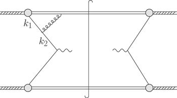
Figure B1. An example of parents of active particles. k1 is a parent of active particles. |
Glauber couplings of these particles are not removed by the summation of final spectators. One may verify that Glauber couplings of k1 eikonalize. It seems that k1 should be defined as active particles even if it does not participate in the hard subprocess directly.
Without loss of generality, let us consider plus-collinear active particles and spectators. Trajectories of these particles originate from the initial plus-collinear hadron and end at the final cuts or the hard vertex. If the plus momentum of a plus-collinear particle k1 flows into the hard vertex finally, then k1 can not survive after the hard collision. In other words, k1 can not be cut by the final cuts even if it does not participate in the hard subprocess directly. For example, one may consider the particle k1 in figure B1. ${k}_{1}^{+}$ flow into the hard vertex through the path k1 → k2 → hard vertex.
According to the above discussions, if there is a path made up of plus-collinear particles k1,…,kn 33(Obviously, ${{ \mathcal P }}^{+}({k}_{j})\gt 0$(1 ≤ j ≤ n) as the reflux of plus momenta, which contradicts classical trajectories of plus-collinear particles, is absent on the leading pinch singular surfaces.) flows into the hard vertex through the path k1 → ⋯ → kn → hard vertex then kj can not be cut by the final cuts and they should be defined as active particles. One may verify the eikonalization of Glauber couplings of kj(1 ≤ j ≤ n). Let us consider the propagator of kj, which reads4.2 .
$\begin{eqnarray}\displaystyle \frac{N(j)}{{k}_{1}^{-}+{l}_{1}^{-}\,+\cdots +\,{l}_{j-1}^{-}+\cdots +\tfrac{{\left({k}_{1\perp }+{l}_{1\perp }\,+\cdots +\,{l}_{j-1\perp }+\cdots \right)}^{2}}{2{{ \mathcal P }}^{+}({k}_{j})}+{\rm{i}}\varepsilon },\end{eqnarray}$
where N(j) represents terms independent of Glauber momenta in the propagator and l1, …lj−1 represent the momenta of Glauber gluons coupling to k1,…,kj−1.34(kj may couple to other non-Glauber particles (except for k1, …kn). We define the momenta of these particles as variables independent of Glauber gluons coupling to kj.) According to the form of the propagators of kj(1 ≤ J ≤ n), poles of l1,…,ln−1 are all located in the lower half plane. Hence one can take the eikonal approximation in Glauber couplings of kj without changing the leading power result. This is compatible with discussions in section It is worth noting that the above definition distinguishes from one’s intuitive insight. For example, let us consider the particle p1 in figure B2.
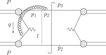
Figure B2. An example of how +-momenta flow affects the definition of plus-collinear active particles and spectators, where the dot line l represents a Glauber gluon. |
At first glance, p1 should be defined as spectators. However, p1 and p2 are defined as active particles if (p1, p2, q) are plus-collinear and ${{ \mathcal P }}^{+}(q)={{ \mathcal P }}^{+}({p}_{1}-{p}_{3})\gt 0$ according to the above discussions since there is a path p1 → p2 → q → hard vertex through which ${p}_{1}^{+}$ and ${p}_{2}^{+}$ flow into the hard vertex. In this case, we choose (p1, l, p3) as independent variables and figure B2 relies on l− through the terms5.2 .) This is compatible with discussions in section 4.2 .
$\begin{eqnarray}\begin{array}{l}\displaystyle \frac{1}{{p}_{1}^{-}+{l}^{-}+\tfrac{{\left({p}_{1\perp }+{l}_{\perp }\right)}^{2}}{2{{ \mathcal P }}^{+}({p}_{1})}+{\rm{i}}\varepsilon }\\ \quad \times \displaystyle \frac{1}{{p}_{1}^{-}+{l}^{-}+\tfrac{{\left({p}_{3\perp }\right)}^{2}}{2{{ \mathcal P }}^{+}({p}_{3})}+\tfrac{{\left({p}_{1\perp }+{l}_{\perp }-{p}_{3\perp }\right)}^{2}}{2{{ \mathcal P }}^{+}({p}_{1}-{p}_{3})}+{\rm{i}}\varepsilon }.\end{array}\end{eqnarray}$
Hence l− is not pinched in the Glauber region at the leading power of λ.35(In fact, figure B2 cancels out in summation over final states as discussed in section For a plus-collinear particle p1 free from the hard vertex, if there are no paths through which ${p}_{1}^{+}$ flow into the hard vertex then p1 flows into the final cuts. There should be a path p1 → ⋯ pn → final cuts. The propagator of pj(1 ≤ j ≤ n − 1) reads
$\begin{eqnarray}\displaystyle \frac{N(j)}{{p}_{1}^{-}+{l}_{1}^{-}\,+\cdots +\,{l}_{j-1}^{-}\,+\cdots +\,\tfrac{{\left({p}_{1\perp }+{l}_{1\perp }\,+\cdots +\,{l}_{j-1\perp }+\cdots \right)}^{2}}{2{{ \mathcal P }}^{+}({p}_{j})}+{\rm{i}}\varepsilon },\end{eqnarray}$
and the final cut on pn reads $\begin{eqnarray}\begin{array}{l}\delta \left({p}_{1}^{-}+{l}_{1}^{-}\,+\cdots +\,{l}_{j-1}^{-}+\cdots \right.\\ \quad \left.+\displaystyle \frac{{\left({p}_{1\perp }+{l}_{1\perp }\,+\cdots +\,{l}_{n-1\perp }+\cdots \right)}^{2}}{2{{ \mathcal P }}^{+}({p}_{n})}\right)\\ \quad =\displaystyle \frac{1}{2\pi }\left(\displaystyle \frac{1}{{p}_{1}^{-}+{l}_{1}^{-}\,+\cdots +\,{l}_{j-1}^{-}\,+\cdots +\,\tfrac{{\left({p}_{1\perp }+{l}_{1\perp }\,+\cdots +\,{l}_{n-1\perp }+\cdots \right)}^{2}}{2{{ \mathcal P }}^{+}({p}_{n})}-{\rm{i}}\varepsilon }\right.\\ \quad \left.-\displaystyle \frac{1}{{p}_{1}^{-}+{l}_{1}^{-}\,+\cdots +\,{l}_{j-1}^{-}\,+\cdots +\,\tfrac{{\left({p}_{1\perp }+{l}_{1\perp }\,+\cdots +\,{l}_{n-1\perp }+\cdots \right)}^{2}}{2{{ \mathcal P }}^{+}({p}_{n})}+{\rm{i}}\varepsilon }\right).\end{array}\end{eqnarray}$
${p}_{j}^{-}$ and pj⊥(1 ≤ j ≤ n) may relies on Glauber momenta. Pinch poles in the Glauber region may originate from the poles of ${p}_{n}^{-}={p}_{1}^{-}+{l}_{1}^{-}\,+\cdots +\,{l}_{j-1}^{-}+\cdot $. Hence Glauber couplings of pj do not eikonalize in general as the Glauber momenta flow into pn finally. We define pj(1 ≤ j ≤ n) as spectators.It is interesting to consider a path including non-collinear particles. For example, we consider a plus-collinear particle p1 and a path p1 → ⋯ → l → ⋯ → pn → hard vertex, where l is soft or ultrasoft or Glauber. Considering that the trajectory of l differs from those of collinear particles, this path should not be viewed as an effective path through which plus momenta of active particles flow into the hard vertex. In fact, Glauber couplings of p1 cancel out if l is soft or ultrasoft according to discussions in section 5.2 since there are non-Glauber interactions after Glauber coupling of p1. In the case that l is Glauber, whether Glauber coupling of p1 eikonalize depends on whether there is a path made up of plus-collinear particles through which ${p}_{1}^{+}$ flow into the hard vertex. In both cases, one should investigate other possible paths made up of plus-collinear particles through which ${p}_{1}^{+}$ flow into the hard vertex.
According to our definition, plus momenta of plus-collinear spectators do not flow into the hard vertex or they flow into the hard vertex through paths including non-collinear particles. In the former case, spectators may survive after the hard collision and the spectators can be cut by the final cuts. That is, inclusive summation over spectators is possible in this case. In the latter case, Glauber couplings of spectators cancel out if the paths include soft or ultrasoft particles as discussed in section 5.2 . If the paths do not contain soft or ultrasoft particles and plus momenta of spectators flow into the hard vertex through Glauber gluons and active particles, we can then deal with Glauber couplings of these spectators according to the skills in sections 4.1 and 5 .
For minus-collinear particles, we have a similar definition.
In summary, we define plus-collinear(minus-collinear) active particles as:36(The two cases may overlap.) (1) the plus-collinear(minus-collinear) particles coupling to particles collinear to other directions or hard modes directly; (2) the plus-collinear(minus-collinear) particles of which the plus (minus) momenta flow into the hard vertex through a path made up of collinear particles. Other plus-collinear(minus-collinear) particles are defined as spectators37(Certainly, a high loop level definition of collinear particles relies on how they couple to other particles and a suitable subtraction scheme which is beyond the scope of this paper.). The definition of active particles is compatible with discussions in section 4.2 . And further, we can deal with Glauber exchanges between spectators and other particles according to skills in sections 4.1 and 5 .
Appendix C. Reparameterization invariance of the effective theory
We consider the reparameterization invariance in this appendix. For simplicity, we neglect ghost fields in this appendix. In original SCET, the reparameterization invariance of the n-collinear sector arises from two types of ambiguity [38, 39]:
| 1. | 1. The subscript p of the collinear fields ξn,p and ${A}_{n,p}^{\mu }$ is arbitrary by order Qλ2 |
| 2. | 2. Transformations on nμ and ${\bar{n}}_{\mu }$ reads $\begin{eqnarray}\begin{array}{l}(a)\left\{\begin{array}{l}{n}_{\mu }\to {n}_{\mu }+{{\rm{\Delta }}}_{\mu }^{\perp }\\ {\bar{n}}_{\mu }\to {\bar{n}}_{\mu }\end{array}\right.\quad (b)\left\{\begin{array}{l}{n}_{\mu }\to {n}_{\mu }\\ {\bar{n}}_{\mu }\to {\bar{n}}_{\mu }+{\varepsilon }_{\mu }^{\perp }\end{array}\right.\\ \quad \times (c)\left\{\begin{array}{l}{n}_{\mu }\to (1+\alpha ){n}_{\mu }\\ {\bar{n}}_{\mu }\to (1-\alpha ){\bar{n}}_{\mu }\end{array}\right.\end{array}\end{eqnarray}$ should not change physical results, where the infinitesimal parameters satisfy the condition $\bar{n}\cdot {{\rm{\Delta }}}^{\perp }=n\cdot {{\rm{\Delta }}}^{\perp }=\bar{n}\cdot {\varepsilon }^{\perp }=n\cdot {\varepsilon }^{\perp }=0$. |
The type-1 transformations leave nμ and ${\bar{n}}^{\mu }$ invariant and affect the subscripts of collinear fields. Keep in mind, the momenta of these particles are independent of the manner which we decompose them. Hence the operators rely on ${{ \mathcal P }}^{\mu }$ and i∂μ through the combination ${{ \mathcal P }}^{\mu }+{\rm{i}}{\partial }^{\mu }$ are invariant under these transformations. At the leading power of λ,7 ) invariant at the leading power of λ.
$\begin{eqnarray}{{ \mathcal P }}^{\mu }+{\rm{i}}{\partial }^{\mu }\simeq \bar{n}\cdot { \mathcal P }{n}^{\mu }+{{ \mathcal P }}_{\perp }^{\mu }+{\rm{i}}n\cdot \partial \end{eqnarray}$
for n-collinear particles and Glauber gluons and $\begin{eqnarray}{{ \mathcal P }}^{\mu }+{\rm{i}}{\partial }^{\mu }\simeq {{ \mathcal P }}^{\mu }\end{eqnarray}$
for soft particles and $\begin{eqnarray}{{ \mathcal P }}^{\mu }+{\rm{i}}{\partial }^{\mu }=i{\partial }^{\mu }\end{eqnarray}$
for ultrasoft particles. Therefore the type-1 transformations leave the action (Table C1. Transformations of relevant operators under the type-2 reparameterization. |
| Type 2a | Type 2b | Type 2c |
|---|---|---|
| ${n}_{\mu }\to {n}_{\mu }+{{\rm{\Delta }}}_{\mu }^{\perp }$ | nμ → nμ | nμ → (1 + α)nμ |
| ${\bar{n}}_{\mu }\to {\bar{n}}_{\mu }$ | ${\bar{n}}_{\mu }\to {\bar{n}}_{\mu }+{\varepsilon }_{\mu }^{\perp }$ | ${\bar{n}}_{\mu }\to (1-\alpha ){\bar{n}}_{\mu }$ |
| $n\cdot {{ \mathcal D }}_{{nG}}\to n\cdot {{ \mathcal D }}_{{nG}}+{{\rm{\Delta }}}^{\perp }\cdot {{ \mathcal D }}_{{nG}}^{\perp }$ | $n\cdot {{ \mathcal D }}_{{nG}}\to n\cdot {{ \mathcal D }}_{{nG}}$ | $n\cdot {{ \mathcal D }}_{{nG}}\to (1+\alpha )n\cdot {{ \mathcal D }}_{{nG}}$ |
| ${{ \mathcal D }}_{{nG}\mu }^{\perp }\to {{ \mathcal D }}_{{nG}\mu }^{\perp }-{{\rm{\Delta }}}_{\mu }^{\perp }\bar{n}\cdot {{ \mathcal D }}_{{nG}}-{\bar{n}}_{\mu }{{\rm{\Delta }}}^{\perp }\cdot {{ \mathcal D }}_{{nG}}^{\perp }$ | ${{ \mathcal D }}_{{nG}\mu }^{\perp }\to {{ \mathcal D }}_{{nG}\mu }^{\perp }-\varepsilon \cdot {{ \mathcal D }}_{{nG}}-{n}_{\mu }{\varepsilon }^{\perp }\cdot {{ \mathcal D }}_{{nG}}^{\perp }$ | ${{ \mathcal D }}_{{nG}\mu }^{\perp }\to {{ \mathcal D }}_{{nG}\mu }^{\perp }$ |
| $\bar{n}\cdot {{ \mathcal D }}_{{nG}}\to \bar{n}\cdot {{ \mathcal D }}_{{nG}}$ | $\bar{n}\cdot {{ \mathcal D }}_{{nG}}\to \bar{n}\cdot {{ \mathcal D }}_{{nG}}+{\varepsilon }^{\perp }\cdot {{ \mathcal D }}_{{nG}}^{\perp }$ | $\bar{n}\cdot {{ \mathcal D }}_{{nG}}\to (1-\alpha )\bar{n}\cdot {{ \mathcal D }}_{{nG}}$ |
| $n\cdot {{ \mathcal D }}_{\bar{n}G}\to n\cdot {{ \mathcal D }}_{\bar{n}G}+{{\rm{\Delta }}}^{\perp }\cdot {{ \mathcal D }}_{\bar{n}G}^{\perp }$ | $n\cdot {{ \mathcal D }}_{\bar{n}G}\to n\cdot {{ \mathcal D }}_{\bar{n}G}$ | $n\cdot {{ \mathcal D }}_{\bar{n}G}\to (1+\alpha )n\cdot {{ \mathcal D }}_{\bar{n}G}$ |
| ${{ \mathcal D }}_{\bar{n}G\mu }^{\perp }\to {{ \mathcal D }}_{\bar{n}G\mu }^{\perp }-{{\rm{\Delta }}}_{\mu }^{\perp }\bar{n}\cdot {{ \mathcal D }}_{\bar{n}G}-{\bar{n}}_{\mu }{{\rm{\Delta }}}^{\perp }\cdot {{ \mathcal D }}_{\bar{n}G}^{\perp }$ | ${{ \mathcal D }}_{\bar{n}G\mu }^{\perp }\to {{ \mathcal D }}_{\bar{n}G\mu }^{\perp }-\varepsilon \cdot {{ \mathcal D }}_{\bar{n}G}-{n}_{\mu }{\varepsilon }^{\perp }\cdot {{ \mathcal D }}_{\bar{n}G}^{\perp }$ | ${{ \mathcal D }}_{\bar{n}G\mu }^{\perp }\to {{ \mathcal D }}_{\bar{n}G\mu }^{\perp }$ |
| $\bar{n}\cdot {{ \mathcal D }}_{\bar{n}G}\to \bar{n}\cdot {{ \mathcal D }}_{\bar{n}G}$ | $\bar{n}\cdot {{ \mathcal D }}_{\bar{n}G}\to \bar{n}\cdot {{ \mathcal D }}_{\bar{n}G}+{\varepsilon }^{\perp }\cdot {{ \mathcal D }}_{\bar{n}G}^{\perp }$ | $\bar{n}\cdot {{ \mathcal D }}_{\bar{n}G}\to (1-\alpha )\bar{n}\cdot {{ \mathcal D }}_{\bar{n}G}$ |
| ${\xi }_{n}\to (1+{{/}\!\!\!\!{{\rm{\Delta }}}}^{\perp }{/}\!\!\!\!{\bar{n}}){\xi }_{n}$ | ${\xi }_{n}\to (1+{{/}\!\!\!\!{\varepsilon }}^{\perp }\tfrac{1}{\bar{n}\cdot {{ \mathcal D }}_{{nG}}}{{/}\!\!\!\!{{ \mathcal D }}}_{{nG}}^{\perp }){\xi }_{n}$ | ξn → ξn |
| ${\xi }_{\bar{n}}\to (1+{{/}\!\!\!\!{{\rm{\Delta }}}}^{\perp }\tfrac{1}{n\cdot {{ \mathcal D }}_{\bar{n}G}}{{/}\!\!\!\!{{ \mathcal D }}}_{\bar{n}G}^{\perp }){\xi }_{\bar{n}}$ | ${\xi }_{\bar{n}}\to (1+{{/}\!\!\!\!{\varepsilon }}^{\perp }{/}\!\!\!\!{n}){\xi }_{\bar{n}}$ | ${\xi }_{\bar{n}}\to {\xi }_{\bar{n}}$ |
| WnG → WnG | ${W}_{{nG}}\to \left(1-\tfrac{1}{\bar{n}\cdot {{ \mathcal D }}_{{nG}}}{\varepsilon }^{\perp }\cdot {{ \mathcal D }}_{{nG}}^{\perp }\right){W}_{{nG}}$ | WnG → WnG |
| ${W}_{\bar{n}G}\to \left(1-\tfrac{1}{n\cdot {{ \mathcal D }}_{\bar{n}G}}{{\rm{\Delta }}}^{\perp }\cdot {{ \mathcal D }}_{\bar{n}G}^{\perp }\right){W}_{\bar{n}G}$ | ${W}_{\bar{n}G}\to {W}_{\bar{n}G}$ | ${W}_{\bar{n}G}\to {W}_{\bar{n}G}$ |
| ψs → ψs | ψs → ψs | ψs → ψs |
| ${A}_{s}^{\mu }\to {A}_{s}^{\mu }$ | ${A}_{s}^{\mu }\to {A}_{s}^{\mu }$ | ${A}_{s}^{\mu }\to {A}_{s}^{\mu }$ |
Where
$\begin{eqnarray}{W}_{{nG}}=\sum _{{perms}}\left(-\displaystyle \frac{g}{\bar{n}\cdot { \mathcal P }}\bar{n}\cdot ({A}_{n,p}+{A}_{{nG},k})\right)\end{eqnarray}$
at leading power of λ. Considering the Glauber exchange causes $n-\bar{n}$ and n-soft correlations, we also present the transformation properties of $\bar{n}$-sector and soft sector in table C1.One may verify that the transformations in table C1 leave the effective action (7 ) invariant at the leading power of λ. Instead of explicit calculations, we would like to show the reason for the invariance. Let us start from the decomposition of the fields2.2 , the subtraction to remove the overlap between AnG and ${A}_{\bar{n}G}$ is not displayed here for simplicity. Although the reparameterization transformations may change fields in the effective theory, the decomposition (C6 ) is invariant under the transformations. Obviously, reparameterization transformations do not mix the (ψoff, Aoff) and (ψn, ψs, ψus, An, As, Aus, AnG). We simply drop the modes (ψoff, Aoff) from the basic theory and obtain the tree-level matching effective action,
$\begin{eqnarray}\begin{array}{rcl}\psi (x) & = & \sum _{n}{\psi }_{n}(x)+{\psi }_{s}(x)+{\psi }_{{us}}(x)+{\psi }_{{off}}(x)\\ {A}^{\mu } & = & \sum _{n}({A}_{n}^{\mu }+{A}_{{nG}}^{\mu })(x)+{A}_{s}^{\mu }(x)+{A}_{{us}}^{\mu }(x)+{A}_{{off}}^{\mu }(x),\end{array}\end{eqnarray}$
where (ψ, Aμ) represent fields in the basic theory and (ψn, ψs, ψus, An, As, Aus, AnG) represent the modes in the effective theory and (ψoff, Aoff) represent the modes we integrate out. As discussed in section $\begin{eqnarray}\begin{array}{rcl}{I}_{{\rm{eff}}} & = & \sum _{n}{\bar{\psi }}_{n}({\rm{i}}{{/}\!\!\!\!{D}}_{{nG}}){\psi }_{n}+\displaystyle \int {{\rm{d}}}^{4}x\displaystyle \frac{1}{2{g}^{2}}{\rm{tr}}\\ & & \times \{[{\rm{i}}{{ \mathcal D }}_{{nG}}^{\mu }+{{gA}}_{n}^{\mu },{\rm{i}}{{ \mathcal D }}_{{nG}}^{\nu }+{{gA}}_{n}^{\nu }]\}{}^{2}\\ & & +{\rm{ghost}}\,{\rm{terms}}\\ & & +{I}_{s}^{G}+{I}_{{us}}+\sum _{n}{I}_{{nG}}\end{array}\end{eqnarray}$
$\begin{eqnarray}+O(\lambda )\end{eqnarray}$
which is invariant under the transformations.We then consider the decomposition7 ). That is to say, the effective action (7 ) is reparameterization invariant at the leading power of λ.
$\begin{eqnarray}\begin{array}{rcl}{\psi }_{n}(x) & = & {\xi }_{n}(x)+{\xi }_{\bar{n}}(x),\quad {\xi }_{n}(x)\equiv \displaystyle \frac{{/}\!\!\!\!{n}{/}\!\!\!\!{\bar{n}}}{2}{\psi }_{n}(x),\\ {\xi }_{\bar{n}}(x) & \equiv & \displaystyle \frac{{/}\!\!\!\!{\bar{n}}{/}\!\!\!\!{n}}{2}{\psi }_{n}(x),\end{array}\end{eqnarray}$
which is reparameterization invariant. We have $\begin{eqnarray}\begin{array}{l}{\bar{\psi }}_{n}({\rm{i}}{{/}\!\!\!\!{D}}_{{nG}}){\psi }_{n}\\ \quad ={\bar{\xi }}_{n}({\rm{i}}{{/}\!\!\!\!{D}}_{{nG}}){\xi }_{n}+{\bar{\xi }}_{\bar{n}}({\rm{i}}{{/}\!\!\!\!{D}}_{{nG}}){\xi }_{n}\\ \quad +{\bar{\xi }}_{n}({\rm{i}}{{/}\!\!\!\!{D}}_{{nG}}){\xi }_{\bar{n}}+{\bar{\xi }}_{\bar{n}}({\rm{i}}{{/}\!\!\!\!{D}}_{{nG}}){\xi }_{\bar{n}}\\ \quad ={\bar{\xi }}_{n}({\rm{i}}n\cdot {D}_{{nG}}){/}\!\!\!\!{\bar{n}}{\xi }_{n}+{\bar{\xi }}_{\bar{n}}({\rm{i}}{{/}\!\!\!\!{D}}_{{nG}}^{\perp }){\xi }_{n}+{\bar{\xi }}_{n}({\rm{i}}{{/}\!\!\!\!{D}}_{{nG}}^{\perp }){\xi }_{\bar{n}}\\ \quad +{\bar{\xi }}_{\bar{n}}({\rm{i}}\bar{n}\cdot {D}_{{nG}}){/}\!\!\!\!{n}{\xi }_{\bar{n}}.\end{array}\end{eqnarray}$
We integrate out ${\xi }_{\bar{n}}$ and have $\begin{eqnarray}\begin{array}{rcl}{\psi }_{n} & = & (1+\displaystyle \frac{1}{\bar{n}\cdot {D}_{{nG}}}{{/}\!\!\!\!{D}}_{{nG}}^{\perp }{/}\!\!\!\!{\bar{n}}){\xi }_{n}\\ & = & (1+{W}_{n}\displaystyle \frac{1}{\bar{{ \mathcal P }}}{W}_{n}^{\dagger }{{/}\!\!\!\!{D}}_{{nG}}^{\perp }{/}\!\!\!\!{\bar{n}}){\xi }_{n}(1+O(\lambda )).\end{array}\end{eqnarray}$
Substituting the expression of ψn(x) into the effective action, we get results equivalent to those in (