


1. Introduction
Heavy-ion collisions at intermediate energies exhibit strong nonequilibrium features and provide a way to study the equation of state, the multi-fragmentation reaction and the production of subthreshold meson [1–4]. The theoretical study of heavy-ion collisions in the intermediate energy region is very difficult due to the combined effects of many factors, such as the mean field, two-body collision and Pauli blocking. For the sake of studying on the dynamics of heavy-ion collision at intermediate energy, theoretical approaches such as extended time-dependent Hartree–Fock theory [5–8] and semi-classical Boltzmann-Uehling-Uhlenbeck (BUU) equation [9, 10] are applied to describe the one-body observable in nuclear collisions. However, since the BUU equation lacks the two-body correlation effects, it cannot be used to describe the properties of the Fermion system far from equilibrium such as multi-fragmentation and subthreshold particle production [11]. There are mainly two kinds of transport approaches for considering the correlation effects between nucleons. One is the quantum molecular dynamics model in which the nucleon is considered to be a gaussian wave packet with a finite width [12–14]. The other is the Boltzmann framework developed based on the BUU model which incorporates fluctuations within the model, such as the Boltzmann–Langevin equation (BLE) which turns many-body problem into one-body problem and considers the dynamical fluctuations caused by many-body associations [11, 15–17]; the stochastic mean field approach which considers dissipation of the relative radial linear momentum [18–20]; and the Boltzmann–Langevin-One-Body dynamics [21, 22]. The first comparison of the fluctuations in transport models is published in 1992 [23]. Up to now, a large number of investigations have been conducted to compare different transport theories to improve the robustness of their predictions. More detailed information on the comparison of transport approaches for heavy-ion collisions can be found in the recent studies and references therein [24–29].
The two-body collision can produce dissipations by random distribution of particle momentum and induce fluctuations by propagating correlations [1]. According to the survey, fluctuation plays an important role in some physical phenomena such as multi-fragmentation and subthreshold particle production [4, 30]. In heavy-ion collisions at the Fermi energy domain up to 150 MeV u−1, the dynamical fluctuations always take place in the early state of the collisions. The fluctuations will naturally propagate along with the self-consistent mean field and particle collisions, rendering the system dynamics reach the unstable region, in which the dynamic instability caused by fluctuations will lead to irreversible events and make the system split into several fragments. Thus, a clear understanding of the reaction mechanism in a quantitative manner needs a microscopic description of the collision process, especially during the strong dissipative region after the contact of projectile and target and begin to overlap [1]. The BLE provides a well-suited method to analyze fragmentation reactions, which incorporates dynamical fluctuations into the collision term of system dynamical evolutions [21]. The addition of dynamical fluctuations creates branching points in the evolution of the system, allowing jumps in different states, including those that are prone to instability, which is important in the fragmentation reactions [31]. The BLE was introduced in 1969 firstly in order to describe the hydrodynamic fluctuations [32, 33]. Ayik and Gregoire et al used the BLE in the non-equilibrium region in the 1980s [11]. The theoretical method applied in this paper is the isospin-dependent Boltzmann–Langevin equation (IBLE) advanced by Xie and Bian, and to which different dynamical fluctuations have been added [34–36].
Nuclear fragmentation is one of the important reaction mechanisms in heavy-ion collisions not only for the finding of new isotopes but also for cosmic-ray physics [37, 38], and still engages continuous interests up to now [39–41]. With the development of radioactive nuclear beam facilities, more exotic isotopes will be found and the heavy-ion and/or hadron therapy will help damage the tumour tissues more effectively [42–44]. In fragmentation reactions at energies ranging from tens of MeV u−1 to hundreds of MeV u−1, a large number of intermediate mass fragments (IMFs) are produced [45, 46]. The process of nuclear fragmentation process can be divided into three stages: dynamical compression and expansion, primary hot nuclear formation and the deexcitation of primary hot nuclear [40]. The intermediate dynamical process of heavy-ion collisions can be well inferred by exploring the properties of these IMFs.
In this study, the dynamical fluctuations in the fragmentation reactions are investigated by using the framework of IBLE. The dynamical fluctuations in momentum space and the effects of different fluctuations on the fragmentation reaction of 112Sn+112Sn are analyzed. The article is organized as follows. The IBLE model and methods are introduced in section 2 , in which we incorporate different fluctuations into the IBLE model and discuss the effects of these fluctuations on dynamical evolution of the system. The calculated results and discussion are presented in section 3 . Finally, conclusions are given in section 4 .
2. Model and methods
2.1. IBLE
The BLE incorporates a fluctuating collision term based on the BUU equation, thus it can describe the dynamical fluctuations originating at the beginning of the collision. The IBLE was obtained by incorporating the isospin effect. The fluctuating single particle density $\hat{f}({\boldsymbol{r}},{\boldsymbol{p}},t)$ is determined by the IBLE [2, 3]:4 ) denote a local ensemble averaging which is generated during a short time interval Δt. When averaging inside one of the subensembles, one is performing a so-called local average [2, 3]. The correlation function C(p1, p2) is improved by Ayik and Gregoire [3, 11], in order to calculate C(p1, p2) directly in non-equilibrium within a weak-coupling approximation. In the semi-classical limit, the correlation function is determined by local averaged single particle density f(r, p, t), which is given by5 ) reflects the ‘fluctuation-dissipation theorem’, that is to say, in phase space, fluctuations and dissipations of single particle density are locally correlated. Another thing should be noted, the IBLE obeys the conservation laws of total particle numbers, momentum and energy [11].
$\begin{eqnarray}\begin{array}{l}(\displaystyle \frac{\partial }{\partial t}+\displaystyle \frac{{\boldsymbol{p}}}{m}\cdot { \triangledown }_{r}-{ \triangledown }_{r}U(\hat{f})\cdot { \triangledown }_{p})\hat{f}({\boldsymbol{r}},{\boldsymbol{p}},t)\\ =\,K(\hat{f})+\delta K({\boldsymbol{r}},{\boldsymbol{p}},t),\end{array}\end{eqnarray}$
in which the left side of the equation presents the Vlasov propagation which is determined by the nuclear mean field $U(\hat{f})$ [47]. On the right side, $K(\hat{f})$ and δK(r, p, t) denote the collision term and fluctuating collision term, respectively [3]. The collision term $K(\hat{f})$ has the usual BUU form but is described by the fluctuating density $\hat{f}({\boldsymbol{r}},{\boldsymbol{p}},t)$, which is: $\begin{eqnarray}\begin{array}{rcl}K({\hat{f}}_{1}) & = & \displaystyle \int {\rm{d}}{{\boldsymbol{p}}}_{2}{\rm{d}}{{\boldsymbol{p}}}_{3}{\rm{d}}{{\boldsymbol{p}}}_{4}W(12;34)\\ & & \left[\times ,\,,[,{\hat{f}}_{3}{\hat{f}}_{4}(1-{\hat{f}}_{1})(1-{\hat{f}}_{2})-{\hat{f}}_{1}{\hat{f}}_{2}(1-{\hat{f}}_{3})(1-{\hat{f}}_{4})\right],\end{array}\end{eqnarray}$
where ${\hat{f}}_{i}$=$\hat{f}({\boldsymbol{r}},{{\boldsymbol{p}}}_{i},t)$ denotes the diagonal elements of single particle density; W(12; 34) is the transition rate which can be described by the cross section for the collision (p1, p2) →(p3, p4) as $\begin{eqnarray}\begin{array}{rcl}W(12;34) & = & \displaystyle \frac{{\rm{d}}\sigma }{{\rm{d}}{\rm{\Omega }}}\delta ({{\boldsymbol{p}}}_{1}+{{\boldsymbol{p}}}_{2}-{{\boldsymbol{p}}}_{3}-{{\boldsymbol{p}}}_{4})\\ & & \times \,\delta ({\epsilon }_{1}+{\epsilon }_{2}-{\epsilon }_{3}-{\epsilon }_{4}),\end{array}\end{eqnarray}$
where εi are the single particle energies. Starting from the two-body correlations, the fluctuating collision term δK(r, p, t) acts as a random force, which is in analogy with the Brownian motion [11, 17]. We cannot calculate the fluctuation collision term explicitly, so we need to introduce approximations like the Markovian approximation [3]. In this description, the fluctuating collision term can be characterized by a correlation function $\begin{eqnarray}\begin{array}{rcl}\langle \delta K({{\boldsymbol{r}}}_{1},{{\boldsymbol{p}}}_{1},{t}_{1})\delta K({{\boldsymbol{r}}}_{2},{{\boldsymbol{p}}}_{2},{t}_{2})\rangle & = & C({{\boldsymbol{p}}}_{1},{{\boldsymbol{p}}}_{2})\delta ({{\boldsymbol{r}}}_{1}-{{\boldsymbol{r}}}_{2})\\ & & \times \,\delta ({t}_{1}-{t}_{2}).\end{array}\end{eqnarray}$
The brackets in equation ( $\begin{eqnarray}\begin{array}{l}C({{\boldsymbol{p}}}_{1},{{\boldsymbol{p}}}_{2})=\displaystyle \int {\rm{d}}{{\boldsymbol{p}}}_{3}{\rm{d}}{{\boldsymbol{p}}}_{4}W(12;34)\left[{f}_{1}{f}_{2}(1-{f}_{3})(1-{f}_{4})\right.\\ \left.+\,{f}_{3}{f}_{4}(1-{f}_{1})(1-{f}_{2})\right]-2\displaystyle \int {\rm{d}}{{\boldsymbol{p}}}_{3}{\rm{d}}{{\boldsymbol{p}}}_{4}W(13;24)\\ \times \,[{f}_{1}{f}_{3}(1-{f}_{2})(1-{f}_{4})+{f}_{2}{f}_{4}(1-{f}_{1})(1-{f}_{3})]\\ +\,\delta ({{\boldsymbol{p}}}_{1}-{{\boldsymbol{p}}}_{2})\displaystyle \int {\rm{d}}{{\boldsymbol{p}}}_{{2}^{{\prime} }}{\rm{d}}{{\boldsymbol{p}}}_{3}{\rm{d}}{{\boldsymbol{p}}}_{4}W({12}^{{\prime} };34)\\ \times \,[{f}_{1}{f}_{{2}^{{\prime} }}(1-{f}_{3})(1-{f}_{4})+{f}_{3}{f}_{4}(1-{f}_{1})(1-{f}_{{2}^{{\prime} }})].\end{array}\end{eqnarray}$
The equation (In this model, the interaction nuclear potential is given as
$\begin{eqnarray}\begin{array}{rcl}{U}_{\tau }(\rho ,\delta ,{\boldsymbol{p}}) & = & \alpha \displaystyle \frac{\rho }{{\rho }_{0}}+\beta {\left(\displaystyle \frac{\rho }{{\rho }_{0}}\right)}^{\gamma }+{E}_{\mathrm{sym}}^{\mathrm{loc}}(\rho ){\delta }^{2}\\ & & +\displaystyle \frac{\partial {E}_{\mathrm{sym}}^{\mathrm{loc}}(\rho )}{\partial \rho }\rho {\delta }^{2}+{E}_{\mathrm{sym}}^{\mathrm{loc}}(\rho )\rho \displaystyle \frac{\partial {\delta }^{2}}{\partial {\rho }_{\tau }}+{U}_{\mathrm{MDI}},\end{array}\end{eqnarray}$
where δ = (ρn − ρp)/ρ is the isospin asymmetry; ρ0 is normal nuclear matter density; ρ = ρp + ρn is the total density with ρp and ρn being the proton and neutron densities, respectively. The ${E}_{\mathrm{sym}}^{\mathrm{loc}}$ is the local part of the symmetry energy, according to [36], we adopt a soft symmetry energy as follows $\begin{eqnarray}{E}_{\mathrm{sym}}^{\mathrm{loc}}(\rho )=\displaystyle \frac{1}{2}{C}_{\mathrm{sym}}{\left(\displaystyle \frac{\rho }{{\rho }_{0}}\right)}^{{\gamma }_{{\rm{s}}}},\end{eqnarray}$
Here we adopt the soft equation of state, which was widely applied in the heavy-ion collisions at intermediate and high incident energies [3, 34]. The UMDI is momentum-dependent potential, which is $\begin{eqnarray}{U}_{\mathrm{MDI}}=\displaystyle \frac{{t}_{4}}{{\rho }_{0}}\int \hat{f}({\boldsymbol{r}},{\boldsymbol{p}}){\left[\mathrm{ln}\left({t}_{5}{\left({\boldsymbol{p}}-{\boldsymbol{p}}^{\prime} \right)}^{2}+1\right)\right]}^{2}{\rm{d}}{{\boldsymbol{p}}}^{{\prime} }.\end{eqnarray}$
The relevant parameters are listed in table 1.Table 1. Parameter set for the IBLE model. |
| K | α | β | γ | Csym | γs | t4 | t5 |
|---|---|---|---|---|---|---|---|
| (MeV) | (MeV) | (MeV) | (MeV) | (MeV) | (MeV−2) | ||
| 200 | −390 | 320 | 1.14 | 29.4 | 0.5 | 1.57 | 0.0005 |
2.2. Numerical simulations
As we have already known, the IBLE incorporates the fluctuating collision term into the BUU equation. The IBLE is consistent with the ‘fluctuation-dissipation theorem’ very well, which denotes that the variable with the largest fluctuation also has the strongest dissipation. In principle, the standard method for solving stochastic differential equations can be used to numerically solve the IBLE equation. However, it is impossible to directly solve the differential equation of the six-dimensional phase space distribution. Where appropriate, rough properties of density fluctuations can be described, and we can use the projection method to numerically simulate IBLE [3]. The fluctuations are projected onto the multipole moments of the momentum distribution, that is, the first and second non-zero terms, quadrupole moment and octupole moment. These fluctuations are eventually added to the momentum distribution locally, which are sufficient to describe the density fluctuations. This multipole moment fluctuation is characterized by a diffusion matrix, which can be obtained by the correlation function $C({\boldsymbol{p}},{{\boldsymbol{p}}}^{{\prime} })$, that is
$\begin{eqnarray}\begin{array}{rcl}{C}_{{{LML}}^{{\prime} }{M}^{{\prime} }}({\boldsymbol{r}},t) & = & \displaystyle \int {\rm{d}}{\boldsymbol{p}}{\rm{d}}{{\boldsymbol{p}}}^{{\prime} }{Q}_{{LM}}({\boldsymbol{p}}){Q}_{{L}^{{\prime} }{M}^{{\prime} }}({{\boldsymbol{p}}}^{{\prime} })C({\boldsymbol{p}},{{\boldsymbol{p}}}^{{\prime} })\\ & = & \displaystyle \int {\rm{d}}{{\boldsymbol{p}}}_{1}{\rm{d}}{{\boldsymbol{p}}}_{2}{\rm{d}}{{\boldsymbol{p}}}_{3}{\rm{d}}{{\boldsymbol{p}}}_{4}\bigtriangleup {Q}_{{LM}}\bigtriangleup {Q}_{{L}^{{\prime} }{M}^{{\prime} }}\\ & & \times W(12,34){f}_{1}{f}_{2}(1-{f}_{3})(1-{f}_{4})\end{array}\end{eqnarray}$
with △QLM = QLM(p1) + QLM(p2) − QLM(p3) − QLM(p4), which is the momentum multipole moment difference of a pair of test particles before and after collisions. QLM(p) is the L-order multipole moment operator with the magnetic quantum number M in the momentum space. f1f2(1 − f3)(1 − f4) describes the Pauli blocking.As can be seen from the above discussion, implementing a dynamical trajectory in the BLE model can have the following steps: (i) At time t, there is a certain single particle density $\hat{f}({\boldsymbol{r}},{\boldsymbol{p}},t)$, and according to the particle simulation of IBLE, the locally averaged density at △t time f(r, p, t + △t) and diffusion matrix ${C}_{{{LML}}^{{\prime} }{M}^{{\prime} }}$ can be obtained. (ii) Calculating the fluctuation of multipole moments of the momentum distribution according to the equation:
$\begin{eqnarray}\begin{array}{rcl}{\hat{Q}}_{{LM}}({\boldsymbol{r}},t+\bigtriangleup t) & = & {Q}_{{LM}}({\boldsymbol{r}},t+\bigtriangleup t)\\ & & +\sum _{{L}^{{\prime} }}\sum _{{M}^{{\prime} }}{\left(\sqrt{\bigtriangleup {tC}({\boldsymbol{r}},t)}\right)}_{{{LML}}^{{\prime} }{M}^{{\prime} }}{W}_{{L}^{{\prime} }{M}^{{\prime} }},\end{array}\end{eqnarray}$
where ${W}_{{L}^{{\prime} }{M}^{{\prime} }}$ is Gaussian random number with mean 0 and variance 1. Here ${\hat{Q}}_{{LM}}$ is the fluctuating multipole moment operator of order L with magnetic quantum number M in the momentum space, while QLM is its locally averaged values. (iii) Finally, fluctuations are inserted back into the single particle density by scaling the local momentum distribution, that is ${Q}_{{LM}}\to {\hat{Q}}_{{LM}}$; f(r, p, t + △t) → $\hat{f}({\boldsymbol{r}},{\boldsymbol{p}},t+\bigtriangleup t)$. This procedure is repeated at each time step of the ensemble events [3, 17].For the sake of applying this method in practice, the multipole moments of the momentum distribution should be truncated to a reasonable size. Some references have simulated the fluctuations at the first two nonvanishing terms, i.e. quadrupole moment and octupole moment [1, 4]. But they hardly analyze the differences between different magnetic quantum numbers. In this paper, the dynamical fluctuations of different multipole moments with different magnetic quantum numbers will be discussed. If we want to achieve fluctuations in the program, a scaling program needs to be added to the program. The algorithm of multipole moments is listed as early as 1984 [48], and the local multipole moments of the momentum distribution are defined as11 ). In this paper, we choose the first two non-vanishing terms, that is quadrupole and octupole moments, and their magnetic quantum numbers components.
$\begin{eqnarray}\begin{array}{rcl}{\hat{Q}}_{{LM}} & = & \sqrt{\displaystyle \frac{16\pi }{2L+1}}{r}^{L}{Y}_{{LM}}(\theta ,\phi ),\\ {Y}_{{LM}}(\theta ,\phi ) & = & {\left(-\right)}^{M}\sqrt{\displaystyle \frac{(2L+1)(L-M)!}{4\pi (L+M)!}}{P}_{L}^{M}(\cos \theta ){{\rm{e}}}^{{\rm{i}}M\phi },\end{array}\end{eqnarray}$
where YLM is the spherical harmonics of order L with magnetic quantum number M, which can be deduced from the associated Legendre polynomial PLM. All the multipole moments of the momentum distribution with different magnetic quantum numbers can be calculated by the equation (2.3. Quadrupole moments of the momentum distribution
At the stage of overlap of the projectile and target, the system exhibits a strong dissipation. This dissipation lasts about 50 fm c−1 and is damping over time. During this period, the two-body collision rate reaches its maximum, which is responsible for the slowing down of the relative motion of two nuclei and for the heating up of the system. The quadrupole moment of the momentum distribution is the first non-vanishing term of the projection method and can be a good observable of the dissipation. It is associated with the single particle distribution $\hat{f}({\boldsymbol{r}},{\boldsymbol{p}},t)$ with11 ). This quadrupole moment has 5 (2L + 1) dimensions. According to the equation (11 ), we can calculate not only the quadrupole moment with magnetic quantum number M = 0, but also the other four quadrupole moments with magnetic quantum number M = − 2, − 1, 1 and 2, which are
$\begin{eqnarray}\begin{array}{rcl}{Q}_{20} & = & \displaystyle \int {\rm{d}}{\boldsymbol{r}}{\rm{d}}{\boldsymbol{p}}{\hat{Q}}_{20}\hat{f}({\boldsymbol{r}},{\boldsymbol{p}},t)\\ & = & \displaystyle \int {\rm{d}}{\boldsymbol{r}}{\rm{d}}{\boldsymbol{p}}(2{{\boldsymbol{p}}}_{z}^{2}-{{\boldsymbol{p}}}_{x}^{2}-{{\boldsymbol{p}}}_{y}^{2})\hat{f}({\boldsymbol{r}},{\boldsymbol{p}},t),\end{array}\end{eqnarray}$
where the beam axis is taken along with the z-axis. The ${\hat{Q}}_{20}$ is the fluctuating quadrupole moment of order L = 2 in momentum space and magnetic quantum number M = 0 which is calculated by the equation ( $\begin{eqnarray}\begin{array}{l}{\hat{Q}}_{2-2}=\displaystyle \frac{\sqrt{6}}{2}({{\boldsymbol{p}}}_{x}^{2}-{{\boldsymbol{p}}}_{y}^{2}),\\ {\hat{Q}}_{2-1}=\sqrt{6}{{\boldsymbol{p}}}_{x}{{\boldsymbol{p}}}_{z},\\ {\hat{Q}}_{21}=-\sqrt{6}{{\boldsymbol{p}}}_{x}{{\boldsymbol{p}}}_{z},\\ {\hat{Q}}_{22}=\displaystyle \frac{\sqrt{6}}{2}({{\boldsymbol{p}}}_{x}^{2}-{{\boldsymbol{p}}}_{y}^{2}).\end{array}\end{eqnarray}$
For heavy-ion collisions at intermediate energy of tens MeV per nucleon, the deformation in momentum space may be described by spheroid, and this deformation can be characterized by different magnetic quantum numbers M. In order to analyze the effects of magnetic quantum numbers on dynamical fluctuations, the different quadrupole moments with different magnetic quantum numbers from M = −2 to M = 2 are calculated. In figure 1, the comparison of the time evolution among Q2M (with the magnetic quantum number M from M = −2 to 2) and among ${C}_{2M2{M}^{{\prime} }}$ (with the magnetic quantum number M from M = −2 to 2, and the same as the magnetic quantum number ${M}^{{\prime} }$) are presented in central 112Sn+112Sn collision at bombarding energy of 60 MeV u−1. The two insets show the magnifications from t = 15 to 45 fm c−1.
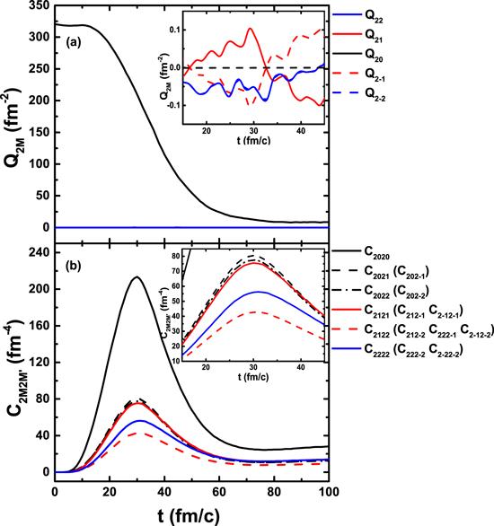
Figure 1. Time evolution of the ensemble-averaged quadrupole moments Q2M (with the magnetic quantum number M from M = −2 to 2) of the momentum distribution (a) and their diffusion coefficients ${C}_{2M2{M}^{{\prime} }}$ (with the magnetic quantum number M from M = −2 to 2, and the same as magnetic quantum number ${M}^{{\prime} }$) (b) in central 112Sn+112Sn collision at bombarding energy of 60 MeV u−1. The two insets show the magnifications from t = 15 to 45 fm c−1. |
From figure 1(a), one can see that the quadrupole moment of the momentum distribution with magnetic quantum number M = 0 evolves from a finite positive value to basically zero and exhibits a strongly dissipative behavior, whereas the quadrupole moments with other magnetic quantum numbers are almost zero from the contact of two nuclei to the late period of collision. This time evolution is easy to understand: at the beginning time of the collision, the pz of two nuclei are naturally positive as the beam axis is taken along with the z-axis, while both the value of px and py are zero, which caused a bump of Q20 and the characteristics of Q2M. Once the two colliding nuclei have merged into one single excited system, the momentum anisotropy has essentially vanished accompanying a thermalization of the system. The diffusion coefficients shown in figure 1(b) exhibit a quite different manner. The ${C}_{2M2{M}^{{\prime} }}$ are almost very small except C2020, all of them exhibit a sizeable peak but others are obviously much smaller than C2020 even at the peak value. For different M and ${M}^{{\prime} }$, there are some ${C}_{2M2{M}^{{\prime} }}$ that are equal. At first, due to the symmetry, the ${C}_{2M2{M}^{{\prime} }}$ equals ${C}_{2{M}^{{\prime} }2M}$ according to equation (9 ), so the diffusion coefficients of these replicates are not presented in the figure. Then, other ${C}_{2M2{M}^{{\prime} }}$ with the same value are listed in parentheses after the ${C}_{2M2{M}^{{\prime} }}$ that are equal to them. At last, it turns out that the cross terms of the diffusion coefficients are much smaller than the non-cross terms except for the ${C}_{2M2{M}^{{\prime} }}$ with $M\cdot {M}^{{\prime} }=0$, because Q20 is large thus resulting in a relatively large cross term of diffusion coefficient. In figure 1(b), one sees that the cross term of the diffusion coefficients C2122 is smaller, while the C2021 and C2022 are larger. Furthermore, the five different quadrupole moments Q2M can degenerate into Q20 and Q2±2 because of the symmetry of the ellipsoid [17]. As a result, the fluctuations of Q20 are larger than those of others, which exhibits that the Q20 of the z-axis is the strongest dissipative variable.
2.4. Octupole moments of the momentum distribution
As can be seen from the above, the influence of Q20 on the dynamical fluctuations is significant especially at the beginning time of the collision. These kinds of fluctuations may affect the whole dynamical process because the equation used in the simulation is nonlinear, while the fluctuations at the end of the collision are not so obvious. In fact, it is the initial fluctuations that affect some reactions like multi-fragmentation and subthreshold particle production.
In further research, the octupole moments of the momentum distribution with different magnetic quantum numbers M = − 3, −2, −1, 0, 1, 2 and 3 are calculated. Just like the quadrupole moment, the octupole moment is also associated with the single particle distribution $\hat{f}({\boldsymbol{r}},{\boldsymbol{p}},t)$. The octupole moments with different magnetic quantum numbers are also calculated according to equation (11 )
$\begin{eqnarray}\begin{array}{rcl}{\hat{Q}}_{3-3} & = & \displaystyle \frac{\sqrt{5}}{2}({{\boldsymbol{p}}}_{x}^{3}-3{{\boldsymbol{p}}}_{x}{{\boldsymbol{p}}}_{y}^{2}),\\ {\hat{Q}}_{3-2} & = & \displaystyle \frac{\sqrt{30}}{2}{{\boldsymbol{p}}}_{z}({{\boldsymbol{p}}}_{x}^{2}-{{\boldsymbol{p}}}_{y}^{2}),\\ {\hat{Q}}_{3-1} & = & \displaystyle \frac{\sqrt{3}}{2}{{\boldsymbol{p}}}_{x}(4{{\boldsymbol{p}}}_{z}^{2}-{{\boldsymbol{p}}}_{x}^{2}-{{\boldsymbol{p}}}_{y}^{2}),\\ {\hat{Q}}_{30} & = & {{\boldsymbol{p}}}_{z}\left(2{{\boldsymbol{p}}}_{z}^{2}-3{{\boldsymbol{p}}}_{x}^{2}-3{{\boldsymbol{p}}}_{y}^{2}\right),\\ {\hat{Q}}_{31} & = & -\displaystyle \frac{\sqrt{3}}{2}{{\boldsymbol{p}}}_{x}(4{{\boldsymbol{p}}}_{z}^{2}-{{\boldsymbol{p}}}_{x}^{2}-{{\boldsymbol{p}}}_{y}^{2}),\\ {\hat{Q}}_{32} & = & \displaystyle \frac{\sqrt{30}}{2}{{\boldsymbol{p}}}_{z}({{\boldsymbol{p}}}_{x}^{2}-{{\boldsymbol{p}}}_{y}^{2}),\\ {\hat{Q}}_{33} & = & -\displaystyle \frac{\sqrt{5}}{2}({{\boldsymbol{p}}}_{x}^{3}-3{{\boldsymbol{p}}}_{x}{{\boldsymbol{p}}}_{y}^{2}).\end{array}\end{eqnarray}$
In figure 2, the comparison of the time evolution among Q3M (with the magnetic quantum number M from M = − 3 to 3) and among ${C}_{3M3{M}^{{\prime} }}$ (with the magnetic quantum number M from M = − 3 to 3, and the same as the magnetic quantum number ${M}^{{\prime} }$) are exhibited in central 112Sn+112Sn collision at bombarding energy of 60 MeV u−1. The two insets show the magnifications from t = 15 to 45 fm c−1. Since the cross terms of the diffusion coefficients with $M\cdot {M}^{{\prime} }\ne 0$ shown above are extraordinarily small, the diffusion coefficients ${C}_{3M3{M}^{{\prime} }}$ are simplified to the non-cross terms and the cross terms with $M\cdot {M}^{{\prime} }=0$. As seen in figure 2(a), the ensemble-averaged value of the total octupole moments is plotted as a function of time, unlike figure 1(a), the octupole moments of the momentum distribution are almost zero throughout the total collision process including the value of magnetic quantum number M = 0, although the Q30 fluctuates in a small range around 0. In figure 2(b), the diffusion coefficient C3030 exhibits a large peak during the most dissipative part of the collision, while other diffusion coefficients do not have so large peak compared to C3030. The large peak of diffusion coefficient C3030 indicates that the value of octupole moment Q30 has an obvious fluctuation before and after the collision, and the ensemble-averaged value of Q30 is almost zero indicating that the value of Q30 has been fluctuating around zero and the range of up and down fluctuations are almost equal. From figure 2(b), one can see that as the magnetic quantum number M increases, the diffusion coefficients C3M3±M decrease, which indicates that the influence of the magnetic quantum number on the fluctuation gradually decreases.
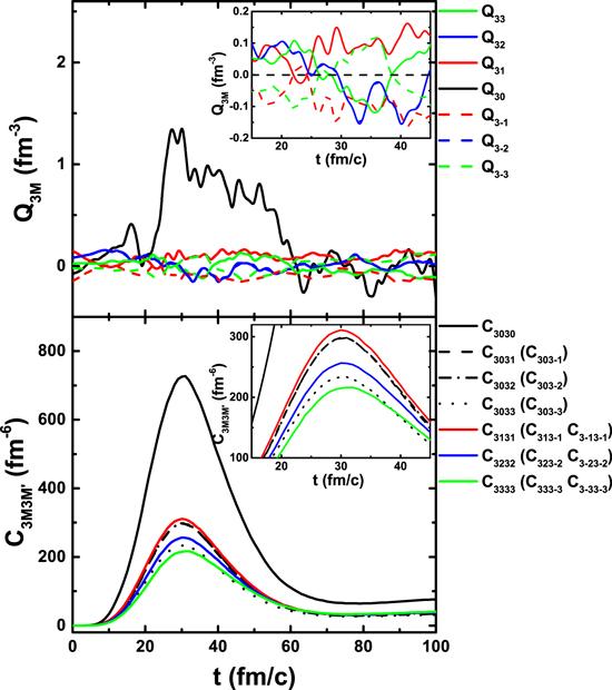
Figure 2. The same as figure 1 but for octupole moments Q3M with the magnetic quantum number M from M = − 3 to 3 in central 112Sn+112Sn collision at bombarding energy of 60 MeV u−1. |
The total comparison between quadrupole moments and octupole moments of the momentum distribution reveals that the dynamical fluctuations of quadrupole moments are dominant during the collision process. In fact, considering the expansion of the multipole moments of momentum distribution, they are constant at both zero and first order due to the conservation of mass and the conservation of momentum. The octupole moments or even higher multipole moments may simply be used as a complement to the quadrupole moment, and considering the local moments of the momentum distribution already corresponds to treat fluctuations as a sort of fluid dynamical level [1]. Therefore, we guess that the dynamical fluctuations are mainly influenced by the quadrupole moments of the momentum distribution and not very sensitive to the higher multipoles.
3. Results and discussion
3.1. Dynamical fluctuations
Since the dynamical fluctuations are mainly influenced by the quadrupole moments of the momentum distribution, as discussed above. In this subsection, the effects of the incident energy on quadrupole moments of the momentum distribution are calculated, and thus the incident energy dependence of the dynamical fluctuations is studied.
Figure 3 presents the time evolutions of the ensemble-averaged quadrupole moments Q20 of the momentum distribution (a), of the corresponding diffusion coefficients C20 (b), of the associated variances σ20 (c), and of the number of colliding particles Ncoll (d) for central 112Sn+112Sn collision at 60 (solid lines), 100 (dashed lines) and 150 (dash–dotted lines) MeV u−1. One can see from the figure, as the incident energy increases, Q20, C20, σ20 and Ncoll become correspondingly larger, revealing that the fluctuations and dissipations become larger. Moreover, when the incident energy increases, the reaction system reaches the maximum fluctuations earlier and the time of the whole reaction process becomes shorter, which can be seen from the time evolution of Ncoll. This is easy to understand, the relative kinetic energy of projectile and target becomes large at high incident energy, which shortens the reaction time. The relative kinetic energy then transforms into the thermal excitation energy, and the reaction system compresses and expands more quickly, thus having a strong dissipation. As can be seen from the figure, at an incident energy of 60 MeV u−1, the fluctuations are strong enough to affect the entire dynamical process of the fragmentation reaction.
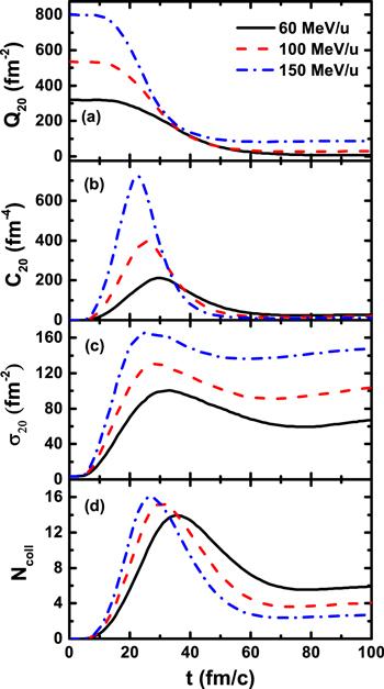
Figure 3. Time evolution of the ensemble-averaged quadrupole moments Q20 of the momentum distribution (a), of the corresponding diffusion coefficients C20 (b), of the associated variances σ20 (c), and of the number of colliding particles Ncoll (d) in central 112Sn+112Sn collision with the incident energy at 60, 100, and 150 MeV u−1. |
The time evolution of the ensemble-averaged quadrupole moments Q20 (a) of the momentum distribution exhibit delaying bumps reflecting a standard dissipation behavior. After the contact of two colliding nuclear, the kinetic energy of the system is gradually transformed into thermal energy at a time of 30–40 fm c−1. The delaying bump of Q20 is caused by the competition of the mean field which flavors an oscillation and the two-body collision which flavors instant relaxation, and it is crucial for the accumulation of the corresponding diffusion coefficient C20 (b) [1]. The early sizeable peak of C20 corresponds to the maximum of the colliding particles Ncoll (d), which is exactly consistent with the fluctuation-dissipation theorem. The associated variances σ20 (c) exhibit sizeable peaks in all incident energies. According to the equation ${\sigma }_{20}=\sqrt{\langle {Q}_{20}^{2}\rangle -\langle {Q}_{20}{\rangle }^{2}}$, the early bump of σ20 reveals that the real Q20 has a big difference with the ensemble-averaged ⟨Q20⟩ when the dissipation is strongest at the beginning of the reaction, which further reflects the presence of a large fluctuation at the beginning of the collision. It is worth noting that these important properties can be expressed on any numerical simulation methods in IBLE.
3.2. Fragmentation reactions
The projection method offers an approximate but very fast method for simulating the IBLE model [1]. In order to analyze the effect of different kinds of dynamical fluctuations on the nuclear fragmentation reactions, in this subsection, the production cross sections of fragments in fragmentation reactions are calculated using different fluctuations. At first the obtained charge distributions of IMFs using different fluctuations are compared with the experimental data [49–51], in order to find the best fluctuations to perform the prediction of fragments generation. Then, the calculated isotopic distributions of fragments are presented.
In fragmentation reactions, we construct clusters using the coalescence model [3, 52, 53], in which particles with relative momenta smaller than P0 and relative distance smaller than R0 are considered to be one cluster [3, 34]. Here we set R0 and P0 are 3.5 fm and 300 MeV c−1, respectively. Simulations are carried out for 10 000 events, and the number of test particles is set at 20.
The calculated charge distributions of IMFs using different dynamical fluctuations in the 40Ca+40Ca reaction at 35 MeV u−1 are shown in figure 4. The solid line, dashed line and dash-dotted line represent the fluctuations of Q20, Q20 + Q22, and Q20 + Q30, respectively. The solid circles show the experimental data [49]. For the experimental data, we note a valley in yield between Z = 3 and 6, and then a more gradual decrease with increasing Z. The calculations using different fluctuations provide a straight falloff in yield with increasing Z, whereas the calculations using Q20 + Q30 fluctuation do provide a significantly better fit to the experimental data. The calculations using Q20 fluctuation lead to a rather poor agreement with the experimental data characterized by underestimating the yield of large charge fragments with Z > 10. But the discrepancy is within an order of magnitude. The results using Q20 + Q22 and Q20 + Q30 fluctuations agree better with the experimental data compared to those using Q20 fluctuation. The yield descends more gently with increasing charge number. However, the simulations using Q20 + Q22 fluctuation overestimate the experimental data at the region of Z < 12. From the figure, we sum up that the octupole moment of the momentum distribution can be used as a complement to the quadrupole moment of the momentum distribution, allowing the calculated results by using Q20 + Q30 fluctuation to better reproduce the experimental data.
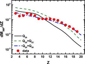
Figure 4. The charge distributions of intermediate mass fragments in the 40Ca+40Ca reaction at 35 MeV u−1 stimulated by IBLE using different dynamical fluctuations, compared with the experimental data [49]. |
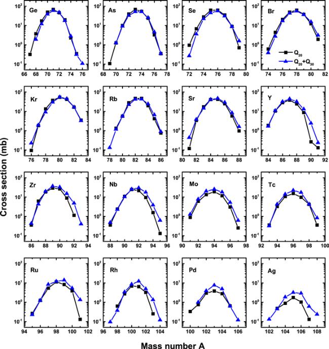
From the early studies, one can conclude that at an incident energy of 60 MeV u−1, the fluctuation is sufficient to influence the dynamical evolution process and allow the system to reach the dynamically unstable region, resulting in fragments formation [3]. Figure 5 displays the calculated isotopic distributions of fragments with 32 ≤ Z ≤ 47 in 112Sn+112Sn reaction at 60 MeV u−1. As shown in figure 5, the square symbols present the cross sections of IBLE with Q20 fluctuation and triangle symbols present the calculations with Q20 + Q30 fluctuation. The overall trends of the production cross sections for fragments using different fluctuations are from up-sloping to down-sloping. The discrepancy between the two kinds of calculations is small in the low charge area shown in the upper two rows of figure 5, and becomes progressively larger from Z = 39. In Q20 + Q30 fluctuation, the fragmentation cross sections are from the lower of Ge element to the higher of Ag element. The fragmentation cross sections by using Q20 fluctuation show the opposite trend. The difference between the cross sections of fragments using Q20 fluctuation and Q20 + Q30 fluctuation is relatively large on the neutron-rich side, with a maximum difference of one order of magnitude.
Figure 5. Calculated isotopic distributions of fragments with 32 ≤ Z ≤ 47 in 112Sn+112Sn reaction at 60 MeV u−1. The square and triangle symbols show the cross sections of fragments using Q20 and Q20 + Q30 fluctuations, respectively. |
In Q20 + Q30 fluctuation, more neutron-rich and proton-rich nuclei like 76Ge, 78Rb, 93Zr, 97Rh, 104Rh, 106Pd, 102Ag and 108Ag are exhibited. However in Q20 fluctuation, only three more proton-rich nuclei are produced, 67Ge, 69As and 100Pd. Thus, we conclude that different dynamical fluctuations have different effects on the cross sections of the fragments produced in the fragmentation reactions. The dynamical fluctuations and dissipations occur at the beginning of the collisions, but they affect the entire collision process including the generation of fragments. The addition of higher multipole moments of the momentum distribution like Q30 always produces more neutron-rich and proton-rich fragments with higher cross sections, especially in the vicinity of the projectile. But with the increase of multipole moments, this effect gradually becomes weaker, which is mainly because the multipole moments become progressively smaller and therefore we truncate the multipole moments to the first two non-vanishing terms Q20 + Q30.
4. Conclusions
In summary, the dynamical fluctuations in the fragmentation reaction of 112Sn+112Sn are investigated in the framework of the IBLE model. The fluctuations are projected onto the multipole moments of the momentum distribution. Based on the time evolutions of quadrupole and octupole moments for different magnetic quantum numbers, it can be seen that Q20 has a strong dissipation, and Q30 and higher multipole moments of the momentum distribution are only used as complements to Q20. The dynamical fluctuations are very sensitive to the incident energy. As the incident energy increases, the dynamical fluctuations become larger, and hence the time to reach the maximum fluctuations and dissipations becomes shorter. In fragmentation reactions, the charge distributions of fragments are calculated using different dynamical fluctuations, and compared with the experimental data. The results using Q20 + Q30 fluctuation have a better agreement with the experimental data. The isotope distributions of fragments show that the use of Q20 + Q30 fluctuation produces more proton-rich and neutron-rich nuclei. And the heavier the fragment charge Z, the larger the difference between the results calculated using Q20 and Q20 + Q30 fluctuations. The results indicate that the dynamical fluctuations mainly occur in the early time of the collisions, and due to the nonlinear nature of the BLE, these fluctuations may affect the whole dynamical process, including the generation of fragments. Large dynamical fluctuations make it possible that the system breaks up into small pieces, thus they can describe appropriately the processes of fragmentation in nuclear collisions. These studies may help to connect the dynamics of heavy-ion collision with the nuclear equation of state and the production of new isotopes. It would be interesting to further investigate the dynamical behaviors of the fluctuations in the future.