


1. Introduction
2. Methodology
2.1. Analytical methods
| i | (i)METEM In accordance with METEM, the following finite series is offered [18–20] $\begin{eqnarray}W(\xi )={a}_{0}+\sum _{j=1}^{M}\left({a}_{j}{{\rm{\Psi }}}^{j}(\xi )+\displaystyle \frac{{b}_{j}}{{{\rm{\Psi }}}^{j}(\xi )}\right),\end{eqnarray}$ for equation (Additionally, the application of METEM requires the function $Psi$(ξ) in equation ( $\begin{eqnarray}D{\rm{\Psi }}-z={{\rm{\Psi }}}^{2},\end{eqnarray}$ that admits the following solution sets $\begin{eqnarray}\begin{array}{rcl}\mathrm{for}\qquad z\lt 0,\qquad {\rm{\Psi }}(\xi ) & = & \left\{\begin{array}{l}-\sqrt{-z}\coth (\sqrt{-z}\xi ),\\ -\sqrt{-z}\tanh (\sqrt{-z}\xi ),\end{array}\right.\\ \mathrm{for}\qquad z\gt 0,\qquad {\rm{\Psi }}(\xi ) & = & \left\{\begin{array}{l}-\sqrt{z}\cot (\sqrt{z}\xi ),\\ \sqrt{z}\tan (\sqrt{z}\xi ).\end{array}\right.\end{array}\end{eqnarray}$ Remarkably, METEM reveals three different types of solutions, including hyperbolic, periodic and irrational solutions. For the hyperbolic and periodic solutions, equation ( |
| ii | (ii)KM According to KM, equation ( $\begin{eqnarray}W(\xi )={a}_{0}+\sum _{j=1}^{M}{a}_{j}{{\rm{\Psi }}}^{j}(\xi ),\end{eqnarray}$ where $M(\in {\mathbb{N}})$ is equally a natural number to be obtained by making a balance between the orders of the highest linear operator, and that of the nonlinear term present; while a0, aj, for j = 1, 2,…,M are unknown constants that would be determined, such that aM ≠ 0, for all M. What's more, KM requires the function $Psi$(ξ) in equation ( $\begin{eqnarray}D{\rm{\Psi }}+{\rm{\Psi }}={{\rm{\Psi }}}^{2},\end{eqnarray}$ such that the following exponential solution is satisfied by the latter equation is given by the function $\begin{eqnarray}{\rm{\Psi }}(\xi )=\displaystyle \frac{1}{1+{{de}}^{\xi }},\end{eqnarray}$ where d is an arbitrary constant. This form of solution expressed in the above equation is basically the only form of solution posed by KM; in comparison with the METEM which gives three types of solutions. |
2.2. NLDM
3. Application
3.1. Analytical methods
| i | (i)METEM With M1 = 1, and M2 = 1, equation ( $\begin{eqnarray}\begin{array}{rcl}{W}_{1} & = & {a}_{0}+{a}_{1}{\rm{\Psi }}(\xi )+\displaystyle \frac{{b}_{1}}{{\rm{\Psi }}(\xi )},\\ {W}_{2} & = & {c}_{0}+{c}_{1}{\rm{\Psi }}(\xi )+\displaystyle \frac{{d}_{1}}{{\rm{\Psi }}(\xi )},\end{array}\end{eqnarray}$ where a0, a1, b1, c0, c1 and d1 are unknown constants to be determined. Therefore, substituting the above solution form into equation ( $\begin{eqnarray*}\begin{array}{l}-2{b}_{1}{d}_{1}{\eta }_{2}k+2{b}_{1}{k}^{2}z-{b}_{1}^{2}{\eta }_{1}k=0,\\ \quad -\,2{b}_{1}{d}_{1}{\lambda }_{2}k+2{d}_{1}{k}^{2}z-{d}_{1}^{2}{\lambda }_{1}k=0,\end{array}\end{eqnarray*}$ $\begin{eqnarray*}\begin{array}{l}{a}_{0}{c}_{1}k{\lambda }_{2}z+{a}_{1}{c}_{0}k{\lambda }_{2}z-{a}_{0}{d}_{1}k{\lambda }_{2}-{b}_{1}{c}_{0}k{\lambda }_{2}\\ -\,{c}_{0}{d}_{1}k{\lambda }_{1}-{{cd}}_{1}+{c}_{0}{c}_{1}k{\lambda }_{1}z+{{cc}}_{1}z=0,\end{array}\end{eqnarray*}$ $\begin{eqnarray*}\begin{array}{l}-{a}_{0}{b}_{1}{\eta }_{1}k+{a}_{1}{c}_{0}{\eta }_{2}{kz}+{a}_{0}{c}_{1}{\eta }_{2}{kz}+{a}_{1}{cz}\\ \quad -\,{a}_{0}{d}_{1}{\eta }_{2}k+{a}_{0}{a}_{1}{\eta }_{1}{kz}-{b}_{1}{c}_{0}{\eta }_{2}k-{b}_{1}c=0,\end{array}\end{eqnarray*}$ $\begin{eqnarray*}\begin{array}{l}-2{b}_{1}{d}_{1}{\eta }_{2}{kz}+2{b}_{1}{k}^{2}{z}^{2}-{b}_{1}^{2}{\eta }_{1}{kz}=0,\\ -\,{a}_{0}{b}_{1}{\eta }_{1}{kz}-{a}_{0}{d}_{1}{\eta }_{2}{kz}-{b}_{1}{c}_{0}{\eta }_{2}{kz}-{b}_{1}{cz}=0,\end{array}\end{eqnarray*}$ $\begin{eqnarray*}\begin{array}{l}-2{b}_{1}{d}_{1}k{\lambda }_{2}z+2{d}_{1}{k}^{2}{z}^{2}-{d}_{1}^{2}k{\lambda }_{1}z=0,\\ -\,{a}_{0}{d}_{1}k{\lambda }_{2}z-{b}_{1}{c}_{0}k{\lambda }_{2}z-{c}_{0}{d}_{1}k{\lambda }_{1}z-{{cd}}_{1}z=0,\end{array}\end{eqnarray*}$ $\begin{eqnarray*}\begin{array}{l}2{a}_{1}{c}_{1}{\lambda }_{2}{kz}+2{c}_{1}{k}^{2}z+{c}_{1}^{2}{\lambda }_{1}{kz}=0,\\ {a}_{0}{c}_{1}k{\lambda }_{2}+{a}_{1}{c}_{0}k{\lambda }_{2}+{c}_{0}{c}_{1}k{\lambda }_{1}+{{cc}}_{1}=0,\end{array}\end{eqnarray*}$ $\begin{eqnarray*}\begin{array}{l}2{a}_{1}{c}_{1}{\eta }_{2}{kz}+2{a}_{1}{k}^{2}z+{a}_{1}^{2}{\eta }_{1}{kz}=0,\\ {a}_{1}{c}_{0}{\eta }_{2}k+{a}_{0}{c}_{1}{\eta }_{2}k+{a}_{1}c+{a}_{0}{a}_{1}{\eta }_{1}k=0,\end{array}\end{eqnarray*}$ $\begin{eqnarray*}\begin{array}{l}2{a}_{1}{c}_{1}{\lambda }_{2}k+2{c}_{1}{k}^{2}+{c}_{1}^{2}{\lambda }_{1}k=0,\\ 2{a}_{1}{c}_{1}{\eta }_{2}k+2{a}_{1}{k}^{2}+{a}_{1}^{2}{\eta }_{1}k=0.\end{array}\end{eqnarray*}$ Now, upon solving the above algebraic system of equations, the unknown constants a0, a1, b1, c0, c1 and d1 are determined as follows $\begin{eqnarray}\begin{array}{cc}{a}_{0}=-\displaystyle \frac{c{\lambda }_{1}-2c{\eta }_{2}}{k\left({\eta }_{1}{\lambda }_{1}-4{\eta }_{2}{\lambda }_{2}\right)}, & {c}_{0}=\displaystyle \frac{2c{\lambda }_{2}-c{\eta }_{1}}{k\left({\eta }_{1}{\lambda }_{1}-4{\eta }_{2}{\lambda }_{2}\right)},\end{array}\end{eqnarray}$ $\begin{eqnarray}\begin{array}{cc}{a}_{1}=-\displaystyle \frac{2\left(2{\eta }_{2}k-k{\lambda }_{1}\right)}{4{\eta }_{2}{\lambda }_{2}-{\eta }_{1}{\lambda }_{1}}, & {c}_{1}=-\displaystyle \frac{2\left({\eta }_{1}k-2k{\lambda }_{2}\right)}{{\eta }_{1}{\lambda }_{1}-4{\eta }_{2}{\lambda }_{2}},\end{array}\end{eqnarray}$ $\begin{eqnarray}\begin{array}{cc}{b}_{1}=\displaystyle \frac{{d}_{1}{\lambda }_{1}-2{d}_{1}{\eta }_{2}}{{\eta }_{1}-2{\lambda }_{2}}, & {d}_{1}={d}_{1},\end{array}\end{eqnarray}$ with $\begin{eqnarray}z=\displaystyle \frac{{d}_{1}\left({\eta }_{1}{\lambda }_{1}-4{\eta }_{2}{\lambda }_{2}\right)}{2k\left({\eta }_{1}-2{\lambda }_{2}\right)}.\end{eqnarray}$ Therefore, this method of solution posed four (4) different sets of solutions via the application of equation ( $\begin{eqnarray}\begin{array}{rcl}{\,}^{1}{w}_{1}(x,t) & = & {a}_{0}-{a}_{1}\sqrt{-z}\coth (\sqrt{-z}({kx}-{ct}))\\ & & -\displaystyle \frac{{b}_{1}}{\sqrt{-z}\tanh (\sqrt{-z}({kx}-{ct}))},\\ {}^{1}{w}_{2}(x,t) & = & {c}_{0}-{c}_{1}\sqrt{-z}\coth (\sqrt{-z}({kx}-{ct}))\\ & & -\displaystyle \frac{{d}_{1}}{\sqrt{-z}\tanh (\sqrt{-z}({kx}-{ct}))},\end{array}\end{eqnarray}$ and $\begin{eqnarray}\begin{array}{rcl}{\,}^{2}{w}_{1}(x,t) & = & {a}_{0}-{a}_{1}\sqrt{-z}\tanh (\sqrt{-z}({kx}-{ct}))\\ & & -\displaystyle \frac{{b}_{1}}{\sqrt{-z}\coth (\sqrt{-z}({kx}-{ct}))},\\ {\,}^{2}{w}_{2}(x,t) & = & {c}_{0}-{c}_{1}\sqrt{-z}\tanh (\sqrt{-z}({kx}-{ct}))\\ & & -\displaystyle \frac{{d}_{1}}{\sqrt{-z}\coth (\sqrt{-z}({kx}-{ct}))},\end{array}\end{eqnarray}$ while for $z=\tfrac{{d}_{1}\left({\eta }_{1}{\lambda }_{1}-4{\eta }_{2}{\lambda }_{2}\right)}{2k\left({\eta }_{1}-2{\lambda }_{2}\right)}\gt 0,$ we get the following wave solutions $\begin{eqnarray}\begin{array}{rcl}{\,}^{3}{w}_{1}(x,t) & = & {a}_{0}-{a}_{1}\sqrt{z}\cot (\sqrt{z}({kx}-{ct}))\\ & & -\displaystyle \frac{{b}_{1}}{\sqrt{z}\tan (\sqrt{z}({kx}-{ct}))},\\ {\,}^{3}{w}_{2}(x,t) & = & {c}_{0}-{c}_{1}\sqrt{z}\cot (\sqrt{z}({kx}-{ct}))\\ & & -\displaystyle \frac{{d}_{1}}{\sqrt{z}\tan (\sqrt{z}({kx}-{ct}))},\end{array}\end{eqnarray}$ and $\begin{eqnarray}\begin{array}{rcl}{\,}^{4}{w}_{1}(x,t) & = & {a}_{0}+{a}_{1}\sqrt{z}\tan (\sqrt{z}({kx}-{ct}))\\ & & +\displaystyle \frac{{b}_{1}}{\sqrt{z}\cot (\sqrt{z}({kx}-{ct}))},\\ {\,}^{4}{w}_{2}(x,t) & = & {c}_{0}+{c}_{1}\sqrt{z}\tan (\sqrt{z}({kx}-{ct}))\\ & & +\displaystyle \frac{{d}_{1}}{\sqrt{z}\cot (\sqrt{z}({kx}-{ct}))}.\end{array}\end{eqnarray}$ Therefore, for k = 0.61, c = 0.25, d1 = 1, and d1 = − 1, we give the three-dimensional (3D) plots for the solution given in equations ( |
| ii | (ii)KM With M1 = 1, and M2 = 1, equation ( $\begin{eqnarray}{W}_{1}={a}_{0}+{a}_{1}{\rm{\Psi }}(\xi ),\qquad {W}_{2}={b}_{0}+{b}_{1}{\rm{\Psi }}(\xi ),\end{eqnarray}$ where a0, a1, b0 and b1 are unknown constants to be determined. Therefore, substituting the above solution form into equation ( $\begin{eqnarray*}\begin{array}{l}-{a}_{1}{b}_{0}{\eta }_{2}k-{a}_{0}{b}_{1}{\eta }_{2}k-{a}_{1}c+{a}_{1}{k}^{2}\\ \quad -\,{a}_{0}{a}_{1}{\eta }_{1}k=0,\end{array}\end{eqnarray*}$ $\begin{eqnarray*}\begin{array}{l}{a}_{1}{b}_{0}{\eta }_{2}k+{a}_{0}{b}_{1}{\eta }_{2}k-2{a}_{1}{b}_{1}{\eta }_{2}k+{a}_{1}c\\ \quad -\,3{a}_{1}{k}^{2}-{a}_{1}^{2}{\eta }_{1}k+{a}_{0}{a}_{1}{\eta }_{1}k=0,\end{array}\end{eqnarray*}$ $\begin{eqnarray*}\begin{array}{l}2{a}_{1}{b}_{1}{\eta }_{2}k+2{a}_{1}{k}^{2}+{a}_{1}^{2}{\eta }_{1}k=0,\ \ -{a}_{1}{b}_{0}{\lambda }_{2}k\\ \quad -\,{a}_{0}{b}_{1}{\lambda }_{2}k-{b}_{1}c+{b}_{1}{k}^{2}-{b}_{0}{b}_{1}{\lambda }_{1}k=0,\end{array}\end{eqnarray*}$ $\begin{eqnarray*}\begin{array}{l}{a}_{1}{b}_{0}{\lambda }_{2}k+{a}_{0}{b}_{1}{\lambda }_{2}k-2{a}_{1}{b}_{1}{\lambda }_{2}k+{b}_{1}c\\ \quad -\,3{b}_{1}{k}^{2}-{b}_{1}^{2}{\lambda }_{1}k+{b}_{0}{b}_{1}{\lambda }_{1}k=0,\end{array}\end{eqnarray*}$ $\begin{eqnarray*}2{a}_{1}{b}_{1}{\lambda }_{2}k+2{b}_{1}{k}^{2}+{b}_{1}^{2}{\lambda }_{1}k=0.\end{eqnarray*}$ Then, on solving the above algebraic system of equations, the unknown constants a0, a1, b0, and b1 are determined as follows $\begin{eqnarray}\begin{array}{rcl}{a}_{0} & = & \displaystyle \frac{\left(c-{k}^{2}\right)\left(2{\eta }_{2}-{\lambda }_{1}\right)}{k\left({\eta }_{1}{\lambda }_{1}-4{\eta }_{2}{\lambda }_{2}\right)},\\ {b}_{0} & = & -\,\displaystyle \frac{\left(c-{k}^{2}\right)\left({\eta }_{1}-2{\lambda }_{2}\right)}{k\left({\eta }_{1}{\lambda }_{1}-4{\eta }_{2}{\lambda }_{2}\right)},\end{array}\end{eqnarray}$ $\begin{eqnarray}\begin{array}{rcl}{a}_{1} & = & -\,\displaystyle \frac{2\left(2{\eta }_{2}k-k{\lambda }_{1}\right)}{4{\eta }_{2}{\lambda }_{2}-{\eta }_{1}{\lambda }_{1}},\\ {b}_{1} & = & -\,\displaystyle \frac{2\left({\eta }_{1}k-2k{\lambda }_{2}\right)}{{\eta }_{1}{\lambda }_{1}-4{\eta }_{2}{\lambda }_{2}},\end{array}\end{eqnarray}$ which yields only one wave solution set which is as follows $\begin{eqnarray}\begin{array}{rcl}{\,}^{1}{w}_{1}(x,t) & = & {a}_{0}+\displaystyle \frac{{a}_{1}}{1+{{d}{\rm{e}}}^{{kx}-{ct}}},\\ {\,}^{1}{w}_{2}(x,t) & = & {b}_{0}+\displaystyle \frac{{b}_{1}}{1+{{d}{\rm{e}}}^{{kx}-{ct}}},\end{array}\end{eqnarray}$ where d is an arbitrary constant. Thus, for d = 0.1, k = 1.5, and c = 0.25, we give the 3D plots for the above solution of the coupled Burger's equation via the application of the KM in figure 3. Again, the solution given in equation ( |
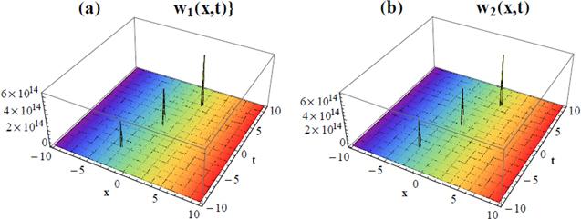
Figure 1. 3D plots for the solution of coupled Burger's equation given in equation ( |
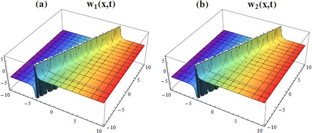
Figure 2. 3D plots for the solution of coupled Burger's equation given in equation ( |
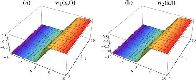
Figure 3. 3D plots for the solution of coupled Burger's equation given in equation ( |
3.2. NLDM
4. Numerical validation
Considering the coupled homogeneous Burger's equation given in equation (
Considering the coupled homogeneous Burger's equation given in equation (
Considering the coupled singular inhomogeneous Burger's equation with [4, 7]
Figure 4. 3D plot for the approximate solution of coupled Burger's equation given in Example |
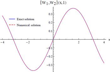
Figure 5. 2D comparison between the exact and approximate solution of coupled Burger's equation given in Example |
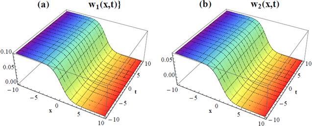
Figure 6. 3D plots for the approximate solution of coupled Burger's equation given in Example |
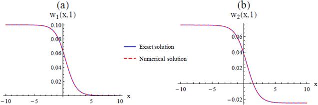
Figure 7. 2D comparisons between the exact and approximate solution of coupled Burger's equation given in Example |
Table 1. Error difference between the exact solution of (w1(x, t), w2(x, t)) and the obtained numerical solution $({{\rm{\Phi }}}_{{1}_{15}},{{\rm{\Phi }}}_{{2}_{15}})$ at t = 1. |
| x | $\left|{w}_{1}(x,t)-{{\rm{\Phi }}}_{{1}_{15}}\right|$ | $\left|{w}_{2}(x)-{{\rm{\Phi }}}_{{2}_{15}}\right|$ |
|---|---|---|
| 0.0 | 0 | 0 |
| 0.1 | 4.51028 × 10⁻¹⁵ | 4.51028 × 10⁻¹⁵ |
| 0.2 | 8.96505 × 10⁻¹⁵ | 8.96505 × 10⁻¹⁵ |
| 0.3 | 1.33366 × 10⁻¹⁴ | 1.33366 × 10⁻¹⁴ |
| 0.4 | 1.75693 × 10⁻¹⁴ | 1.75693 × 10⁻¹⁴ |
| 0.5 | 2.16493 × 10⁻¹⁴ | 2.16493 × 10⁻¹⁴ |
| 0.6 | 2.54796 × 10⁻¹⁴ | 2.54796 × 10⁻¹⁴ |
| 0.7 | 2.90601 × 10⁻¹⁴ | 2.90601 × 10⁻¹⁴ |
| 0.8 | 3.23630 × 10⁻¹⁴ | 3.23630 × 10⁻¹⁴ |
| 0.9 | 3.53606 × 10⁻¹⁴ | 3.53606 × 10⁻¹⁴ |
| 1.0 | 3.79696 × 10⁻¹⁴ | 3.79696 × 10⁻¹⁴ |
Table 2. Error difference between the exact solution of (w1(x, t), w2(x, t)) and the obtained numerical solution $({{\rm{\Phi }}}_{{1}_{20}},{{\rm{\Phi }}}_{{2}_{20}})$ at t = 1. |
| x | $\left|{w}_{1}(x,t)-{{\rm{\Phi }}}_{{1}_{3}}\right|$ | $\left|{w}_{2}(x)-{{\rm{\Phi }}}_{{2}_{3}}\right|$ |
| 0.0 | 7.00966 × 10⁻⁵ | 7.00966 × 10⁻⁵ |
| 0.1 | 7.20085 × 10⁻⁵ | 7.20085 × 10⁻⁵ |
| 0.2 | 7.35479 × 10⁻⁵ | 7.35479 × 10⁻⁵ |
| 0.3 | 7.467 97 × 10−5 | 7.46797 × 10⁻⁵ |
| 0.4 | 7.53775 × 10⁻⁵ | 7.53775 × 10⁻⁵ |
| 0.5 | 7.56246 × 10⁻⁵ | 7.56246 × 10⁻⁵ |
| 0.6 | 7.54151 × 10⁻⁵ | 7.54151 × 10⁻⁵ |
| 0.7 | 7.47540 × 10⁻⁵ | 7.47540 × 10⁻⁵ |
| 0.8 | 7.36572 × 10⁻⁵ | 7.36572 × 10⁻⁵ |
| 0.9 | 7.21502 × 10⁻⁵ | 7.21502 × 10⁻⁵ |
| 1.0 | 7.02674 × 10⁻⁵ | 7.02674 × 10⁻⁵ |