


1. Introduction
Quantum key distribution (QKD) can share secure keys between two legitimate parties (Alice and Bob) across an unsecured quantum channel where an eavesdropper (Eve) might exist [1–3]. There are two categories of protocols for the implementation, which are called discrete-variable (DV) QKD [4] and continuous-variable (CV) QKD [5]. A CV-QKD technique based on the Gaussian-modulated coherent states (GMCS) protocol has been proposed as an alternative solution to DV-QKD [6, 7], which eliminates the barrier to implementing required specialized hardware, such as a single-photon detector and source. It can transmit the secret key by modulating the quadrature components of the optical field and utilizing heterodyne or homodyne detection, which has demonstrated security under both coherent attacks [8] and collective attacks [9]. Gratifyingly, many studies have been put forward to improve the transmission performance [10–12]. On the other hand, the development of the technique of wavelength division multiplexing [13] shows a viable way to use a single coherent communication system to implement both classical communication and CV-QKD.
Recently, a novel scheme known as simultaneous QKD and classical communication (SQCC) was proposed, which is an attractive scheme due to the similarity of the hardware required for implementing classical coherent optical communication and the GMCS QKD in practice [14]. To achieve better performance, impressive developments in terms of the classical carrier phase estimation (CPE) technique [15] and a plug-and-play configuration [16] have been achieved to simplify the complexity of the SQCC system in fiber channels. Moreover, techniques of using measurement-device-independent (MDI) QKD [17, 18] were proposed to prevent all potential attacks on side-channel attacks caused by practical detectors, compared with point-to-point (PP) CV-QKD via Bell-state detection on an untrustworthy third party (Charlie). Furthermore, the sending-or-not-sending twin-field (SNS-TF) QKD protocol was reported to tolerate a large misalignment error rate [19]. Based on the SNS-TF QKD, a field-test QKD over 428 km of deployed commercial fiber was demonstrated [20], and a task of 511 km long-haul fiber trunk linking two distant metropolitan areas was completed [21]. The results, which provide a new distance record, bridge the gap between laboratory and applications and pave the way for large-scale fiber quantum networks across cities with MDI QKD.
Intriguingly, an improved Kalman filter method [22] over the satellite-mediated link was proposed to extend the SQCC scheme to the employment of free space, which shows its potential to develop a range of global applications. Moreover, the first free space MDI QKD over a 19.2 km urban atmospheric channel was realized [23], and a decoy-state BB84 in MDI QKD was used [24], which opened the way for long-distance MDI QKD in free space.
However, as part of constructing a worldwide network without fiber constraints [25], we also need to value the cruciality of underwater SQCC for ocean development and modern communications. This can provide a more secure approach compared with the traditional acoustic technique in the military field, such as in submarines, ocean sensor networks, and various ocean vehicles. Unfortunately, there is still a lack of research on underwater simultaneous two-way classical communication and QKD (STCQ) MDI communication.
Against this background, we analyse the feasibility and security of STCQ MDI transmittance, where legitimate partners exchange a series of classical bits concurrently in the pure ocean channel. By analysing the encoding combination, we detail the protocol and demonstrate the feasibility of communicating with legitimate partners to exchange classical data concurrently. To estimate the transmittance of diverse ocean depths, we consider the probability distribution transmittance (PDT) for the underwater channel, including the random ellipse light model caused by the atmospheric turbulence and the influence of the extinction coefficient based on existing marine chlorophyll data. We perform numerical simulations to determine the optimal modulation variance for low bit error rates (BERs) of 10−9 while maintaining a positive secret key rate (SKR). Furthermore, we also take into consideration the SKR under finite-size effects and show the feasibility of our proposed scheme in practical scenarios. Our work shows the significance of choosing the appropriate transmission depth and modulation variance according to the different types of oceans on Earth, paving the way for practical implementation of the underwater STCQ scheme.
This paper is organized as follows. In section 2 , detailed descriptions of the protocol conceived are given. In section 3 , we calculate the SKR for the STCQ protocol under the performance of a low BER of 10−9 with consideration of the influence of the probability distribution of the transmittance, and numerical simulations based on experimental system parameters are provided with discussions of related trends in performance. Finally, we conclude this paper in section 4 .
2. Implementation of the STCQ protocol
This section shows the details of the proposed STCQ scheme over the ocean channel, and a measurement result analysis of classical bit transmission is performed.
2.1. Description of the protocol
Due to the equivalence of the prepare-and-measure (PM) method and entanglement-based (EB) method, we adopt the PM STCQ scheme to simplify the undersea description of the protocol. The quadrature phase-shift keying (QPSK) description and the STCQ protocol shown in figures 1(a) and (b) are described as follows.
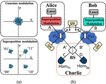
Figure 1. (a) Phase-space representations of various coherent communication schemes. QPSK, quadrature phase-shift keying. (b) Prepare-and-measure (PM) scheme of STCQ protocol. STCQ, simultaneous two-way classical and quantum; Hom1x(2p), homodyne detection of measuring the $X\left(P\right)$ quadrature; BS: 50:50 beam splitter; QM, quantum memory; $\alpha ,$ modulated signal amplitude of two-way classical communication. |
Step 1. Alice prepares her encoded classical bits $\{{m}_{A},{n}_{A}\}$ and Gaussian random numbers with zero means and a variance of ${V}_{A}$ on a coherent state $\left|\left({x}_{A}-\tfrac{\alpha }{\sqrt{2}}{{\rm{e}}}^{-{\rm{i}}\pi {m}_{A}}\right)+{\rm{i}}\left({p}_{A}-\tfrac{\alpha }{\sqrt{2}}{{\rm{e}}}^{-{\rm{i}}\pi {n}_{A}}\right)\right\rangle .$ Meanwhile, Bob prepares $\left|\left({x}_{B}-\tfrac{\alpha }{\sqrt{2}}{{\rm{e}}}^{-{\rm{i}}\pi {m}_{B}}\right)+{\rm{i}}\left({p}_{B}-\tfrac{\alpha }{\sqrt{2}}{{\rm{e}}}^{-{\rm{i}}\pi {n}_{B}}\right)\right\rangle $ with zero means and a variance of ${V}_{B}$ encoded by classical bits $\{{m}_{B},{n}_{A}\}$ to convey the classical ciphertext bits. After encoding and preparing, Alice and Bob send their coherent states to Charlie through different oceanic quantum channels with lengths ${L}_{AC}$ and ${L}_{BC},$ respectively.
Step 2. The coherent states from Alice and Bob interfere at a balanced beam splitter (BS). Both the $X$ quadrature and $P$ quadrature are measured by using Bell-state measurement [26] as ${X}_{C}=\tfrac{{X}_{A}-{X}_{B}}{\sqrt{2}},\,{P}_{C}=\tfrac{{P}_{A}+{P}_{B}}{\sqrt{2}}.$ Then Charlie broadcasts the measurement results $\{{X}_{C},{P}_{D}\}.$
Step 3. After receiving the measurement results $\{{X}_{C},{P}_{D}\},$ Alice and Bob decode each other's data, respectively, based on the measurement findings and the data supplied by themselves. Then Bob removes the classical displacement as ${X}_{B}={x}_{B}+k{X}_{C},{P}_{B}={p}_{B}+k{P}_{C}$ to obtain the Gaussian data associated with the secret key. $k$ is the amplification coefficient related to channel loss, which is described as $k=g/\sqrt{\displaystyle \frac{{V}_{B}-1}{{V}_{B}+1}}$ in the equivalent EB scheme [17], $g$ is the gain of displacement, and ${V}_{B}$ is related to the variance Gaussian modulation. The details above are calculated in appendix C .
Step 4. Alice and Bob perform parameter estimation via an authenticated public channel, information reconciliation, and privacy amplification to share the secret key.
In practice, the EB scheme usually easily performs security analysis. The EB scheme of the STCQ protocol shown in figure 2(b) comprises the following steps: First, Alice and Bob prepare entanglement resources EPR1 and EPR2 with variances of VA and VB, respectively. Then, they keep modes A1 and B1, and send the other modes A2 and B2 to Charlie through the underwater channel. After that, Charlie receives modes A2 and B2 and performs Bell-state measurement detection, and broadcasts the measurement results through the classical channel publicly. According to the data announced, Bob modifies mode B1 to B1' by a displacing operation with a gain of g, and the mode of Alice remains. Ultimately, Alice measures mode A1, and Bob measures mode B1' to obtain the final data by heterodyne detection.
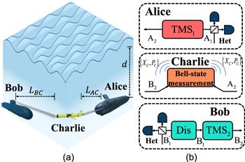
Figure 2. (a) Scenario of STCQ-based underwater submarine communication; one of the motherships releases an unmanned undersea vehicle as the repeater without exposing the risk. (b) Entanglement-based (EB) scheme of STCQ protocol. TMS, two-mode squeezed state; Het, heterodyne detection; Dis, displacement operation. |
2.2. Results of the measurement
The scheme can realize two-way classical communication while completing the distribution of quantum keys. To represent the features and benefits of this coding accurately, we analyse the measurement results from Charlie's side. Note that the analysis does not imply that it is possible to prove the security of Alice's and Bob's sending when doing two-way classical communication. For the convenience of demonstration, we suppose that Alice and Bob have no information leakage in the process of sending to Charlie, and Eve can only intercept the information that Charlie broadcasts to the outside world. Here are nine different measurements, as shown in figure 3, which are related to the Bell detection and the encoding method in figure 1(a). After receiving the results published by the untrusted third party Charlie, Alice and Bob can locate the corresponding combination according to the data sent by themselves, further inferring the other party's data. For example, as soon as Alice knows that Charlie has announced the ‘grey' combination after she has sent the code ‘11', she knows Bob has sent the ‘11' as well. So Bob knows, based on the combination result. However, even though Eve knows the measurement result, she cannot infer the users' classical bits by precisely guessing two ‘grey' combinations between $\left\{11,11\right\}$ and $\left\{01,01\right\}.$

Figure 3. Nine different measurement results are mapped in the phase space and classified by order (I), (II), and (IV). The number of times each color's measurement result appears in (a) is represented by these orders. In terms of the measurement findings, the transmitter and receiver are symmetric. |
A variety of colored blocks have been used to mark the Bell-state measurement results to explore the characteristics of two-way classical communication further. Moreover, we use three sequence numbers (I), (II), and (IV) to classify the number of times that the measurement result of the different colored blocks appears in figure 4, and the colored blocks with an order corresponding to the measurement results in figure 3.
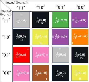
Figure 4. Combination of the results based on the Bell-state measurement. |
To begin with, we will concentrate on the type of (I), which appears just once in figure 4. This means that once Eve has tapped the measurement results, she knows the transmission combinations equivalently. Eve must, however, guess the particular sent bits of each user with a probability of 50%. More specifically, the results red_$1/\sqrt{2}(\alpha ,\alpha )$ result from the combination codes $\left\{11,01\right\},$ but the particular sent bits of Alice could be either ‘11' or ‘01' and Bob for ‘01' or ‘11' correspondingly, plus green_$1/\sqrt{2}(-\alpha ,\alpha )$ from $\left\{01,11\right\},$ brown_$1/\sqrt{2}(\alpha ,-\alpha )$ from $\left\{10,00\right\},$ and orange_$1/\sqrt{2}(-\alpha ,-\alpha )$ form $\left\{00,10\right\}.$
Next, we focus on the type of (II), which indicates that the corresponding measurement results are twofold. Eve has to predict not just each user's unique transmitted bits but also the sorts of possible combinations. For example, the combination pink_$1/\sqrt{2}(\alpha ,0)$ may have resulted from the combination codes $\left\{11,00\right\}$ or $\left\{10,01\right\}.$ Furthermore, Eve has a lower probability of 25% to guess whether the bits of Alice (Bob) are ‘11', ‘00', ‘10', or ‘01'. It is also similar to the combination purple_$1/\sqrt{2}(-\alpha ,0),$ where Alice (Bob) could send ‘01', ‘10', ‘00', or ‘11'. Notably, the bits transmitted by Alice and Bob on the diagonal of the results matrix are identical, giving Eve a 50% chance of achieving the codes, such as the gray_$1/\sqrt{2}(0,\alpha )$ resulting from the combination codes either $\left\{11,11\right\}$ or $\left\{01,01\right\},$ and the yellow_$1/\sqrt{2}(0,-\alpha )$ resulting from the combination codes either $\left\{10,10\right\}$ or $\left\{00,00\right\}.$
Furthermore, we examine the type of (IV), which signifies that the corresponding measurement results appear four times. There is only black_$1/\sqrt{2}(0,0)$ resulting from the combination codes $\left\{11,10\right\},$ $\left\{10,11\right\},$ $\left\{01,00\right\},$ or $\left\{01,00\right\}$ shown in table A1. Due to their symmetrical nature, Eve also only has a probability of 25% of achieving the transmission bits of ‘11', ‘10', ‘01', or ‘01' on the side of Alice (Bob).
However, the situations above are only the result of transmitting a single data set. If a series of bits are transmitted, the probability of Eve's achieving will decrease exponentially with the increase of the code length, which means the security increases as the length of the transmission sequence increases. For instance, if a series of measures are pink_$1/\sqrt{2}(\alpha ,0)$ and purple_$1/\sqrt{2}(-\alpha ,0)$ sequentially, the transfer combination might be $\left\{11,00\right\}$ or $\left\{10,01\right\}$ initially, followed by $\left\{01,10\right\}$ or $\left\{00,11\right\}.$ Thus, Eve has only the probability of 6.25% of achieving Alice's transmitted bits from ‘1101', ‘1110', ‘1100', ‘1111', ‘0001', ‘0010', ‘0000', ‘0011', ‘1001', ‘1010', ‘1000', ‘1011', ‘0101', ‘0110', ‘0100', and ‘0111'.
Based on the above analysis and classification results, we can deduce the probability that Eve correctly deduces the coding sequence from Charlie's broadcasting $P({S}_{{\rm{crt}}}),$ which has the form
$\begin{eqnarray}P({S}_{{\rm{crt}}})={\left[\displaystyle \sum _{i=1}^{9}p({R}_{(i)}){\left({A}_{{N}_{(i)}}^{1}\right)}^{-1}\right]}^{n},\end{eqnarray}$
where $p({R}_{(i)})$ is the probability of measured combination results when transmitting a random sequence, and ${N}_{(i)}$ is the number of specific bits corresponding to the measurement result, as shown in figure 4. Moreover, ${\left({A}_{N}^{M}\right)}^{-1}\,=\left(N-M\right)!/N!,$ and the length of the coding transition sequence is $n.$ Therefore, the results are shown in figure 5.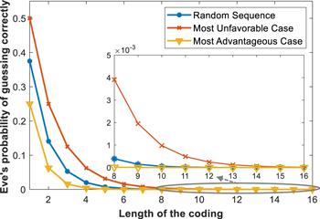
Figure 5. Probability that Eve correctly deduces the coding sequence with length $n.$ For comparison, we assume that the user transmits the easiest and hardest guessable bits all the time in the most unfavorable and the most advantageous case, respectively. |
3. Performance analysis
In this section, the BER of two-way classical communication and the PDT are considered to determine the SKR of STCQ protocol. Subsequently, we show the performance of our proposed scheme compared to the original CV-MDI QKD scheme.
3.1. Derivation of the secret key rate
Unlike the quantum channels in fibers with fixed attenuation coefficients, SKR is affected by the transmission fluctuation in the oceanic fading channel.
The attenuation properties of seawater vary significantly between oceans, mainly owing to differences in its composition. Even within the exact location, the attenuation effect varies according to the ocean's depth and the transmission distance. Beer's law [27, 28] can be used to estimate total extinction losses asA .
$\begin{eqnarray}{T}_{{\rm{ext}}}={{\rm{e}}}^{-C(\lambda ,d)L},\end{eqnarray}$
where $L$ is the horizontal transmission distance and the total attenuation coefficient $C(\lambda ,d)$ is the function of the wavelength $\lambda $ and the depth $d,$ which is noted in appendix Moreover, we consider the regular refraction in turbulence changes, which are connected to temperature and salinity fluctuations, and follow the statistics of turbulent scalar fields. The probability distribution for oceanic transmittance is applied, including beam shape deformation, beam wandering, and beam-broadening effects. This model, dubbed the elliptic beam approximation, applies to weak and strong turbulence, covering most of the regimes seen in underwater communication situations [29].
The transmittance $T$ can be calculated in the Monte Carlo simulation by [30]2 ), and ${T}_{0}$ indicates the transmittance without the effects of beam wandering and extinction, which is given in appendix B . Other parameters are related to the shape of the ellipse model of beam sources, which is shown in figure B1.
$\begin{eqnarray}T={T}_{{\rm{ext}}}{T}_{0}\exp \left\{-{\left[\displaystyle \frac{r/a}{R\left(2/{W}_{{\rm{eff}}}(\varphi -\phi )\right)}\right]}^{{\rm{\Lambda }}\left(2/{W}_{{\rm{eff}}}^{(\varphi -\phi )}\right)}\right\},\end{eqnarray}$
where the extinction transmittance ${T}_{{\rm{ext}}}$ is denoted in equation (In addition, the modulation variance has to be optimized before we calculate the SKR. We take the BER of ${10}^{-9}$ achieved in the experiment in a phase-shift keying communication system based on optical homodyne as the computational requirement [31], which the details are given in appendix C , and the required signal amplitude $\alpha $ of STCQ can be expressed as
$\begin{eqnarray}\begin{array}{l}\alpha ={\text{erfc}}^{-1}\left(2{c}_{{\rm{BER}}}\right){\left\{1-{\left[{\text{erfc}}^{-1}\left(2{c}_{{\rm{BER}}}\right)\right]}^{2}{\sigma }_{\phi }/{\sigma }_{s}\right\}}^{-1/2}\\ \,\times \sqrt{\displaystyle \frac{\left\langle {T}_{A}\right\rangle {\eta }_{{\rm{\hom }}}({\varepsilon }_{0A}+{V}_{{\rm{MA}}})+\left\langle {T}_{B}\right\rangle {\eta }_{{\rm{\hom }}}({\varepsilon }_{0B}+{V}_{{\rm{MB}}})+2\left(1+{v}_{{\rm{el}}}\right)}{\left(\left\langle {T}_{A}\right\rangle +\left\langle {T}_{B}\right\rangle \right){\eta }_{{\rm{\hom }}}}},\end{array}\end{eqnarray}$
where ${{\rm{erfc}}}^{-1}$ represents the inverse complementary error function, ${\eta }_{{\rm{\hom }}}$ is the homodyne detection efficiency, and ${\sigma }_{\phi }$ and ${\sigma }_{s}$ are the extra-noise variance and shot-noise variance, respectively. Moreover, ${\varepsilon }_{0A}$ and ${\varepsilon }_{0B}$ are the excess noise of Alice and Bob, and $\left\langle {T}_{A}\right\rangle $ and $\left\langle {T}_{B}\right\rangle $ denote the estimated channel mean transmittance of Alice or Bob, respectively.If we assume that Bob's two-mode compressed states and the displacement operation are untrustworthy, the STCQ protocol's equivalent EB scheme is turned into a general one-way CV QKD model. As a result, the lower limit key rate of CV-MDI QKD qualifies the SKR inferred from the common one-way CV QKD. In the case of reverse reconciliation, the asymptotic SKR $K$ of the CV-MDI QKD under optimum collective attack is given by [6]C , and the secure key rate $R$ can be further written as
$\begin{eqnarray}K=\beta {I}_{{\rm{AB}}}-{\chi }_{{\rm{BE}}},\end{eqnarray}$
where $\beta $ is the reconciliation efficiency, ${I}_{{\rm{AB}}}$ denotes Alice and Bob's Shannon mutual information, and ${\chi }_{{\rm{BE}}}$ represents the maximum accessible information between Eve and Bob, which is the Holevo bound. The details above are calculated in appendix $\begin{eqnarray}\begin{array}{l}K=\beta {\mathrm{log}}_{2}\left[\displaystyle \frac{{T}_{{\rm{AB}}}{V}_{{\rm{MA}}}+1+{T}_{{\rm{AB}}}\left(1+{\chi }_{{\rm{t}}}\right)}{1+{T}_{{\rm{AB}}}\left(1+{\chi }_{{\rm{t}}}\right)}\right]\\ \,-G\left(\displaystyle \frac{{\lambda }_{1}-1}{2}\right)-G\left(\displaystyle \frac{{\lambda }_{2}-1}{2}\right)+G\left(\displaystyle \frac{{\lambda }_{3}-1}{2}\right),\end{array}\end{eqnarray}$
where $G(\ast )=(\ast +1){\mathrm{log}}_{2}(\ast +1)-\ast {\mathrm{log}}_{2}\ast $ related to the von Neumann entropy, and ${\lambda }_{{\rm{i}}}$ are the symplectic eigenvalues of the covariance matrices. Moreover, ${T}_{{\rm{AB}}}$ represents the total quantum channel transmittance between Alice and Bob.Furthermore, the SKR above is achieved in the asymptotic regime under idealized simplification assumptions in the asymptotic limit of infinite data size. In practical scenarios, a pair of legal users cannot exchange an infinite number of signals, implying that the secret key has a finite length [32]. Naturally, a part of the exchanged signals has to be used for parameter estimation due to the unidentifiable characteristics of the quantum channel [16].
Under the finite-size regime, the SKR ${K}_{{\rm{FSR}}}$ is given by6 ), and the other details are shown in appendix C .
$\begin{eqnarray}{K}_{{\rm{FSR}}}=\displaystyle \frac{{\mathscr{N}}}{ {\mathcal M} }\left[K-{\rm{\Delta }}({\mathscr{N}})\right],\end{eqnarray}$
where $ {\mathcal M} $ represents the total number of signals exchanged by Alice and Bob during the scheme when they use ${\mathscr{N}}$ signals to generate the keys, where half of the $\left( {\mathcal M} -{\mathscr{N}}\right)$ signals will be used in parameter estimation. $K$ is the asymptotic key rate in equation (3.2. Numerical simulations
In the following, the modulation variance is optimized before we show the simulation results of our STCQ protocol based on the oceanic turbulence at the low BER of 10−9. As a result, we focus on the SKR and amplitude as a function of the modulation variance over various transmission distances, showing two different application scenarios in the oceans S2 and S5 in figure 6. Furthermore, we set the simulated depth of transmission at 75 m for the sake of avoiding the range of absorption peaks, in which $d\in \left[92,{\rm{1}}06\right]$ m for S2 and $d\in \left[31,{\rm{62}}\right]$ m for S5, which can be seen in figures A1 and B2.
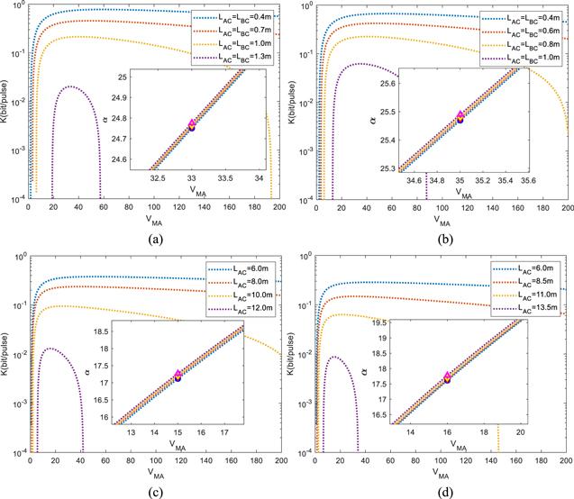
Figure 6. Secret key rate (SKR) (main graph) and amplitude of the classical signal (inset graph) as a function of the modulation variance in the symmetric scenario where the BER is less than 10−9 on oceans S2 for (a) and S5 for (b) and in the asymmetric scenario where the BER is less than 10−9 on oceans S2 for (c) and S5 for (d). Other simulation parameters are set as follows: the extra noise in two channels that is independent of the amplitude of the classical signal ${\varepsilon }_{{\rm{0A}}}={\varepsilon }_{{\rm{0B}}}=0.002,$ the detector efficiency ${\eta }_{{\rm{\hom }}}=0.98,$ the electronic noise ${\nu }_{{\rm{el}}}=0.01,$ the phase-noise variance ${\sigma }_{\phi }={10}^{-6},$ and the reconciliation efficiency $\beta =0.98.$ |
In the symmetric cases, Charlie is positioned directly in the middle of the two senders (${L}_{{\rm{AC}}}={L}_{{\rm{BC}}}$), which favors the use of the star topology [33]. However, when the transmission distance increases, the transmission loss increases rapidly because the postprocessing step is asymmetric when Bob modifies his data and Alice keeps hers, which cannot result in the system's best performance, as shown in figure 6.
We can note that the longer the transmission distance, the narrower the range of near-optimal modulation variance, and the lower the SKR becomes. Moreover, in the symmetric cases, the optimal modulation variances of oceans S2 and S5 are 33 and 35, respectively, which are reached around the peak of SKR. The optimal modulation variance's corresponding amplitude values are about 24.75 and 25.48 for oceans S2 and S5, respectively, as presented in the inset graphs of figures 6(a) and (b). The relationship between modulation variance and amplitude can also be verified from equation (4 ). The curves in the illustration are nearly coincident for different transmission distances and for the sake of the PDT are included in both the denominator and numerator simultaneously.
Analogously, we can plot the SKR and amplitude as a function of the modulation variance over various transmission distances in the extremely asymmetric case, where Charlie is very close to Bob (${L}_{{\rm{BC}}}\approx 0$), as shown in figures 6(c) and (d). The optimal modulation variance's corresponding amplitude values are about 17.25 and 17.75 for oceans S2 and S5, respectively, when the optimal modulation variances are 15 and 16. The distinction is that the appropriate range of modulation variance is wider in the extremely asymmetric case than in the symmetric scenario compared to the equivalent transmission distances.
Consequently, the flexibility of optional modulation variance gives it superiority in long-distance communication, which is suitable for point-to-point transmission. On the other hand, the comparison of the secure key rate will be shown in the next part.
As previously discussed, we undertake numerical simulations of the asymptotic SKR of STCQ QKD in symmetric and asymmetric instances at oceans S2 and S5 under the constraint of a low BER of 10−9 in classical communication. The modulation variance has been optimized, and the modulation variances are taken as 33 at S2 and 35 at S5 in symmetric and 15 at S2 and 16 at S5 in asymmetric scenarios, respectively, as shown in figure 6. Figure 7 presents the simulation results, while the Pirandola–Laurenza–Ottaviani–Banchi (PLOB) bound [34] of the SKR of direct transmission over lossy bosonic channels and the SKR of original Gaussian CV-MDI QKD [17] are also plotted for comparison.
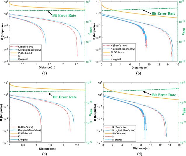
Figure 7. SKR as a function of the transmission distance in the symmetric scenario at oceans S2 for (a) and S5 for (b), and in the extremely asymmetric scenario at oceans S2 for (c) and S5 for (d), where the BER is less than 10−9. For comparison, the SKR following Beer's law (dotted line), considered the nonturbulence channel, is computed based on the same parameters of the turbulence channel (solid line). Other simulation parameters are set as follows: the extra noise in two channels that is independent of the amplitude of the classical signal ${\varepsilon }_{{\rm{0A}}}={\varepsilon }_{{\rm{0B}}}=0.002,$ the detector efficiency ${\eta }_{{\rm{\hom }}}=0.98,$ the electronic noise ${\nu }_{{\rm{el}}}=0.01,$ the phase-noise variance ${\sigma }_{\phi }={10}^{-6},$ and the reconciliation efficiency $\beta =0.98.$ |
According to the numerical simulation results, the gap between the proposed STCQ protocol and the original CV-MDI QKD scheme in symmetric scenarios is shorter than in the asymmetric cases, whether in the ocean S2 or S5, where the original protocol is more in tune with the PLOB bound (the solid line). The STCQ protocol, on the other hand, is capable of enabling concurrent two-way classical communication and CV-MDI QKD with just a slight performance degradation, which is only minor degradation of about 0.08 m and 0.04 m in terms of the maximum distance at SKR of 10−4 bit/pulse on oceans S2 and S5, respectively, in the symmetric scenarios.
Moreover, while the BER gradually increases with transmission distance in the asymmetric case, which is more sensitive than the symmetric case, it is always less than our goal BER of 10−9. It is also shown that the positivity and necessity of choosing appropriate modulation variance and optimization based on different ocean types and application scenarios. It is worth noting that the curve of the SKR is slightly undulated in the case of transmitting a relatively further distance, as shown in figures 7(b) and (d) on the asymmetric scenario. This can be attributed to the transmission fluctuations [35] in the oceanic fading channel.
In addition, figure 8 shows the SKR in the finite-size regime of the asymmetric configuration. For comparison, different block lengths ${\mathscr{N}}$ and the asymptotic regime are also plotted.

Figure 8. Finite-size key rates of the STCQ protocol of the asymmetric scenario in ocean S2 for (a) and S5 for (b). Other simulation parameters are set the same as in figure 7. |
4. Conclusions
In this paper, we have proposed an STCQ protocol for fluctuating oceanic channels and investigated regular extinction and random turbulence effects based on real-data modelling of chlorophyll concentration and numerical simulation via the Monte Carlo method respectively. Our numerical simulations choose ocean S2 and ocean S6 as objects of study, which have different transmittance and absorption peaks of 92 m and 57 m, respectively. This result shows the importance of choosing the appropriate transmission depth depending on the ocean type for submarines, where the valley range of the PDT will seriously affect the transmission distance. In addition, performance simulations have shown that the asymmetric scenario is superior to the symmetric case both in desirable transmission distance and in selecting the optimal modulation variance. Furthermore, we have taken into account the finite-size effect to accommodate the practical implementation. It can be seen that the fewer signals exchanged, the more pronounced the finite-size impact is, and the more rapidly the SKR and security transmission distance decrease. As the block length ${\mathscr{N}}$ increases from 105 to 109, more signals may be used to estimate parameters and extract keys, and the SKR approaches the asymptotic value. These results show a feasible way to apply our proposed scheme to the ocean scenario, which demonstrates the potential of sea, land, and air integrated communication, making the STCQ extend to a broader range of worldwide applications.
Appendix A. Regular extinction coefficient
In general, the profile shape parameters change with the chlorophyll concentration on the surface, which causes difficulty in coefficient determination. A study experimentally quantified the parameters using 2419 distinct chlorophyll profiles [36]. The ocean's location on Earth was classified into several serial groups equivalently, each of which corresponded to a specific range of chlorophyll concentrations near the surface. A complete list of the parameters for each above is given in table A1.
Table A1. Parameter values for S1–S6 oceans [36]. |
| ${\rm{Tpyes}}$ | $\begin{array}{l}{c}_{{\rm{chl}}}\\ ({\rm{mg}}\,{{\rm{m}}}^{-3})\end{array}$ | $\begin{array}{l}{c}_{{\rm{bkg}}}\\ ({\rm{mg}}\,{{\rm{m}}}^{-3})\end{array}$ | $\begin{array}{l}S(\times {10}^{-3})\\ ({\rm{mg}}\,{{\rm{m}}}^{-3})\end{array}$ | H (mg) | dmax (m) |
|---|---|---|---|---|---|
| S1 | 0.708 | 0.0429 | −0.103 | 11.87 | 115.4 |
| S2 | 1.055 | 0.0805 | −0.260 | 13.89 | 92.01 |
| S3 | 1.485 | 0.0792 | −0.280 | 19.08 | 82.36 |
| S4 | 1.326 | 0.1430 | −0.539 | 15.95 | 65.28 |
| S5 | 1.557 | 0.2070 | −1.030 | 15.35 | 46.61 |
| S6 | 3.323 | 0.1600 | −0.705 | 24.72 | 33.03 |
What follows demonstrate the effect of the STCQ scheme on the underwater CV-QKD system. The regular extinction of an optical signal produced by seawater absorption and scattering across various ocean types and the probability density function of transmittance using the ellipse model are also considered. The total attenuation coefficient is given as
$\begin{eqnarray}C(\lambda ,d)={C}_{{\rm{sca}}}(\lambda ,d)+{C}_{{\rm{abs}}}(\lambda ,d),\end{eqnarray}$
where ${C}_{{\rm{sca}}}(\lambda ,d)$ and ${C}_{{\rm{abs}}}(\lambda ,d)$ are the factors of scattering and absorption respectively, which are affected by the concentration of chlorophyll-a, fulvic and humic acid absorption.Chlorophyll-a refers to phytoplankton, fulvic acid, and humic acid is the nutrient for phytoplankton. Therefore, the absorption coefficient in the chlorophyll-a-based model can be given by
$\begin{eqnarray}\begin{array}{l}{C}_{{\rm{abs}}}(\lambda ,d)={a}_{w}(\lambda )+{a}_{f}{C}_{f}(d)\exp \left(-{k}_{f}\lambda \right)\\ \,+{a}_{h}{C}_{h}(d)\exp \left(-{k}_{h}\lambda \right)+{a}_{c}{\left[{C}_{c}(d)/{c}_{c}\right]}^{0.602},\end{array}\end{eqnarray}$
where ${a}_{w}(\lambda )$ is the absorption coefficient of pure water in proportion to the wavelength $\lambda $ [37]. ${C}_{c}(d)$ is the concentration of chlorophyll-a (${c}_{c}=1\,{\rm{mg}}\,{{\rm{m}}}^{-3}$) given in the following. We chose a wavelength of 530 nm to minimize losses in the 450–550 nm transmission window on seawater [38]. The scattering coefficient, which is affected by pure water and particulate matter scattering, also follows a similar form: $\begin{eqnarray}{C}_{{\rm{sca}}}(\lambda ,d)={b}_{w}(\lambda )+{b}_{s}{C}_{s}(d)+{b}_{l}{C}_{l}(d),\end{eqnarray}$
where ${b}_{w}=0.005826{(400/\lambda )}^{4.322}$ is the coefficient of the scattering spectrum for pure water. Moreover, the other specific parameters are coefficients of fulvic acid, humic acid, and the scattering coefficient of small and large particulate matter.In the chlorophyll-a-based model, various biological characteristics determine the spectra of the absorption and scattering spectra, which are classified according to their optical properties. For absorption in equation (A1 ), ${a}_{f}=35.959\,{{\rm{m}}}^{2}\,{{\rm{mg}}}^{-1}$ and ${a}_{h}=18.828\,{{\rm{m}}}^{2}\,{{\rm{mg}}}^{-1}$ are the specific absorption coefficient of fulvic acid and humic acid, respectively; ${k}_{f}=0.0189\,{{\rm{nm}}}^{-1}$ and ${k}_{h}=0.01105\,{{\rm{nm}}}^{-1}$ are the fulvic acid and humic acid exponential coefficients, respectively. The concentration of fulvic acid ${C}_{f}(d)$ and the concentration of humic acid ${C}_{h}(d)$ are related to the one-parameter model for attenuation and have the form
$\begin{eqnarray}{C}_{f}(d)=1.74098{C}_{c}(d)\exp \left(0.12327{C}_{c}(d)\right),\end{eqnarray}$
$\begin{eqnarray}{C}_{h}\left.(d\right)=0.19334{C}_{c}(d)\exp \left(0.12343{C}_{c}(d)\right),\end{eqnarray}$
where ${C}_{c}(d)$ is the concentration of chlorophyll-a, which can be can be modelled at a depth $d$ as a Gaussian curve with five numerically determined parameters as [39] $\begin{eqnarray}{C}_{c}(d)={c}_{{\rm{bkg}}}+Sd+\displaystyle \frac{H}{\sigma \sqrt{2\pi }}\exp \left[\displaystyle \frac{-{\left(d-{d}_{\max }\right)}^{2}}{2{\sigma }^{2}}\right],\end{eqnarray}$
where ${c}_{{\rm{b}}{\rm{k}}{\rm{g}}}$ is the chlorophyll concentration at the surface in the background, $S$ is the vertical gradient of concentration, which is negative because to the gradual loss of chlorophyll with depth, $H$ is the amount of chlorophyll that exceeds the background level, ${d}_{\max }$ is the depth of the deep chlorophyll maximum (DCM), and the standard deviation $\sigma $ is given by $\begin{eqnarray}\sigma =\displaystyle \frac{H}{\sqrt{2\pi \left[{c}_{{\rm{chl}}}\left({d}_{\max }\right)-{c}_{{\rm{bkg}}}-S{d}_{\max }\right]}},\end{eqnarray}$
and the concentration of small particles ${C}_{s}(d)$ and large particles ${C}_{l}(d)$ are given by the following equations: $\begin{eqnarray}{C}_{s}(d)=0.01739{C}_{c}(d)\exp \left(0.11631{C}_{c}(d)\right),\end{eqnarray}$
$\begin{eqnarray}{C}_{l}(d)=0.76284{C}_{c}(d)\exp \left(0.03092{C}_{c}(d)\right).\end{eqnarray}$
The distribution of extinction coefficient $C(\lambda ,d)$ as a function of submarine depth $d$ for S1–S6 is plotted in figure A1. The above sections discussed two distinct ocean quality types: the S2 ocean (the red solid line) and the S5 ocean (the green solid line), in which the extinction coefficient reaches its maximum value at depths of 92 m and 47 m, respectively. Generally, a submersible's operating range is limited to a few hundred meters. We limit our numeral calculations to depths of 200 m in both oceans for analytical purposes.
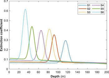
Figure A1. Extinction coefficient of extinction as a function of submarine depth including absorption and scattering in various ocean types. The S1–S6 oceanic parameters are given in table A1. |
Appendix B. Elliptic-beam model
The theory of quantum light propagation via the atmosphere is well researched, with the atmosphere being regarded as a quantum channel with fluctuating transmission [40]. When the loss fluctuation is assumed to be a valid random variable, the theory also agrees rather well with the log-normal model [28], as demonstrated in Canary Islands studies [41], and overcomes the inherent inconsistency of physical properties [29].
Due to the random property of oceanic turbulence channels and atmospheric turbulence channels being similar [42], the quasi-probabilistic Glauber–Sudarshan $P$ function can be given to describe the PDT in oceanic turbulence as
$\begin{eqnarray}{P}_{{\rm{out}}}(\alpha )=\displaystyle {\int }_{0}^{1}{\rm{d}}T{\mathscr{P}}(T)\displaystyle \frac{1}{T}{P}_{{\rm{in}}}\left(\displaystyle \frac{\alpha }{\sqrt{T}}\right),\end{eqnarray}$
where ${P}_{{\rm{out}}}$ and ${P}_{{\rm{in}}}$ are the output and input $P$ functions, respectively, ${T}_{A\left(B\right)}$ being the intensity transmittance of Alice or Bob given by $\begin{eqnarray}{T}_{A\left(B\right)}=\displaystyle {\int }_{{\mathscr{S}}}{{\rm{d}}}^{2}rI(r;L),\end{eqnarray}$
where ${\mathscr{S}}$ is the aperture area, $I(r;L)$ is the normalized intensity, and with respect to the full plant $r=\{x,y\}.$ In general, ocean turbulence acts as a loss source for transmitted photons, which are detected at the receiver by a sensor module with a restricted aperture when a Gaussian beam that propagates along the z-axis onto the aperture plane at distance $z=L$ is taken into our consideration.The irregular losses are induced by the displacement of the beam centroid caused by beam wandering and the redistribution of energy throughout the beam section caused by beam widening and deformation. Furthermore, the receiving beam is expected to have an elliptical profile in the elliptic beam model and can be described using a random vector as $v=\left({x}_{0},{y}_{0},{{\rm{\Theta }}}_{1},{{\rm{\Theta }}}_{2}\right).$ In the received aperture, $({x}_{0},{y}_{0})$ are the beam-centroid coordinates of the incoming beam, ${\rm{\Theta }}$ denotes the consequences of beam broadening and elliptic deformation, and ${{\rm{\Theta }}}_{1}=\,\mathrm{ln}({w}_{1}/{w}_{0}),$ ${{\rm{\Theta }}}_{2}=\,\mathrm{ln}({w}_{2}/{w}_{0}),$ where the ellipse semi-axes are ${w}_{1}$ and ${w}_{2}$ with the initial beam radius ${w}_{0},$ as depicted in figure B1.
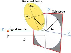
Figure B1. Schematic of an ellipse model. In this model, the beam source is deformed from the transmission distance of $L$ with ellipse semi-axes ${w}_{1}$ and ${w}_{2},$ where $a$ and $r$ represent the aperture radius and the beam-deflection distance, respectively. |
The Monte Carlo method was used to apply the Kolmogorov power spectrum to maritime turbulence and estimate ${\mathscr{P}}(T),$ are shown as follows. Based on the above, the mean values of vector $v$ have the form [43]
$\begin{eqnarray}v=\left(\left\langle {x}_{0}\right\rangle ,\left\langle {y}_{0}\right\rangle ,\left\langle {{\rm{\Theta }}}_{1}\right\rangle ,\left\langle {{\rm{\Theta }}}_{2}\right\rangle \right),\end{eqnarray}$
with the covariance matrix given by $\begin{eqnarray}{\rm{\Sigma }}=\left(\begin{array}{llll}\left\langle {\rm{\Delta }}{x}_{0}^{2}\right\rangle & 0 & 0 & 0\\ 0 & \left\langle {\rm{\Delta }}{y}_{0}^{2}\right\rangle & 0 & 0\\ 0 & 0 & \left\langle {\rm{\Delta }}{{\rm{\Theta }}}_{1}^{2}\right\rangle & \left\langle {\rm{\Delta }}{{\rm{\Theta }}}_{1}{\rm{\Delta }}{{\rm{\Theta }}}_{2}\right\rangle \\ 0 & 0 & \left\langle {\rm{\Delta }}{{\rm{\Theta }}}_{1}{\rm{\Delta }}{{\rm{\Theta }}}_{2}\right\rangle & \left\langle {\rm{\Delta }}{{\rm{\Theta }}}_{1}^{2}\right\rangle \end{array}\right).\end{eqnarray}$
By applying the classical Kolmogorov power spectrum on underwater turbulence [44], the parameters of $v$ and ${\rm{\Sigma }}$ can be calculated as
$\begin{eqnarray}\left\langle {\rm{\Delta }}{x}_{0}^{2}\right\rangle =\left\langle {\rm{\Delta }}{y}_{0}^{2}\right\rangle =27.12{\zeta }^{4/5}{\omega }^{-4/15}{k}^{-1/15}{L}^{37/15},\end{eqnarray}$
where the wave number $k=2\pi /\lambda ,$ $L$ indicates the distance between the transmitter plane and the receiver plane. Moreover, $\zeta $ and $\omega $ are the dissipation rate of temperature or salinity variance and the kinetic energy dissipation rate, respectively, which are considered constant at a given depth for a horizontal link [45]. We focus on the strong turbulence, which has more effect on beam-wandering ($\zeta \in \left[{10}^{-11},{10}^{-10}\right],$ $\omega \in \left[{10}^{-5},{10}^{-3}\right]$). Typically, we can simulate strong and weak oceanic turbulence by updating the values of $\zeta $ and $\omega $ ($\zeta {\omega }^{-1/3}={10}^{-14}$), which is smaller than the strong turbulence case ($\zeta {\omega }^{-1/3}={10}^{-12}$) [46]. The consequences of beam broadening and elliptic deformation can be given as $\begin{eqnarray}\left\langle {{\rm{\Theta }}}_{i}\right\rangle =\,\mathrm{ln}\left(\displaystyle \frac{{\left[{q}_{1}{{\rm{\Phi }}}_{1}^{3}-{q}_{2}{{\rm{\Phi }}}_{1}^{2}+ {\mathcal F} +{ {\mathcal F} }^{-1}\right]}^{2}}{\sqrt{{\left[1+{ {\mathcal F} }^{2}+\left({q}_{1}{{\rm{\Phi }}}_{1}-{q}_{2}\right){{\rm{\Phi }}}_{1}^{2} {\mathcal F} \right]}^{2}+{q}_{3}{{\rm{\Phi }}}_{2}}}\right),\end{eqnarray}$
$\begin{eqnarray}\left\langle {\rm{\Delta }}{{\rm{\Theta }}}_{i}^{2}\right\rangle =\,\mathrm{ln}\left(1+\displaystyle \frac{{q}_{4}{{\rm{\Phi }}}_{2}}{{\left[1+{ {\mathcal F} }^{2}+\left({q}_{1}{{\rm{\Phi }}}_{1}-{q}_{2}\right){{\rm{\Phi }}}_{1}^{2} {\mathcal F} \right]}^{2}}\right),\end{eqnarray}$
$\begin{eqnarray}\left\langle {\rm{\Delta }}{{\rm{\Theta }}}_{1}{\rm{\Delta }}{{\rm{\Theta }}}_{2}\right\rangle =\,\mathrm{ln}\left(1+\displaystyle \frac{{q}_{5}{{\rm{\Phi }}}_{2}{ {\mathcal F} }^{-2}}{{\left[{q}_{1}{{\rm{\Phi }}}_{1}^{3}-{q}_{2}{{\rm{\Phi }}}_{1}^{2}+ {\mathcal F} +{ {\mathcal F} }^{-1}\right]}^{2}}\right),\end{eqnarray}$
where $ {\mathcal F} =k{w}_{0}/2L$ is the Fresnel parameter, ${q}_{1}=131.4,$ ${q}_{2}=54.06,$ ${q}_{3}=248.99,$ ${q}_{4}=1009.81,$ ${q}_{5}=49.95,$ and ${{\rm{\Phi }}}_{1}={\zeta }^{2/5}{\omega }^{-2/15}{k}^{7/15}{L}^{11/15},$ ${{\rm{\Phi }}}_{2}={\zeta }^{6/5}{\omega }^{-2/5}{k}^{7/5}{L}^{11/5} {\mathcal F} (1+{ {\mathcal F} }^{2}).$The transmittance without the effects of beam wandering and extinction ${T}_{0}$ has the form
$\begin{eqnarray}\begin{array}{l}{T}_{0}=1-{ {\mathcal I} }_{0}\left[{a}^{2}\left(\displaystyle \frac{1}{{W}_{1}^{2}}-\displaystyle \frac{1}{{W}_{2}^{2}}\right)\right]\exp \left[-{a}^{2}\left(\displaystyle \frac{1}{{W}_{1}^{2}}+\displaystyle \frac{1}{{W}_{2}^{2}}\right)\right]\\ \,-2\left\{1-\exp \left[-\displaystyle \frac{{a}^{2}}{2}{\left(\displaystyle \frac{1}{{W}_{1}}-\displaystyle \frac{1}{{W}_{2}}\right)}^{2}\right]\right\}\\ \,\times \exp \left\{-{\left[\displaystyle \frac{{\left({W}_{1}+{W}_{2}\right)}^{2}/\left|{W}_{1}^{2}-{W}_{2}^{2}\right|}{R\left(\displaystyle \frac{1}{{W}_{1}}-\displaystyle \frac{1}{{W}_{2}}\right)}\right]}^{{\rm{\Lambda }}\left(\displaystyle \frac{1}{{W}_{1}}-\displaystyle \frac{1}{{W}_{2}}\right)}\right\},\end{array}\end{eqnarray}$
where ${\rm{\Lambda }}(\ast )$ and $R(\ast )$ are the scale and shape functions, which have the form $\begin{eqnarray}\begin{array}{l}{\rm{\Lambda }}(\ast )=2{a}^{2}{\ast }^{2}\displaystyle \frac{\exp \left(-{a}^{2}{\ast }^{2}\right){ {\mathcal I} }_{1}\left({a}^{2}{\ast }^{2}\right)}{1-\exp \left(-{a}^{2}{\ast }^{2}\right){ {\mathcal I} }_{0}\left({a}^{2}{\ast }^{2}\right)}\\ \,\times \left\{\mathrm{ln}\left[2\displaystyle \frac{1-\exp \left(-\displaystyle \frac{1}{2}{a}^{2}{\ast }^{2}\right)}{1-\exp \left(-{a}^{2}{\ast }^{2}\right){ {\mathcal I} }_{0}\left({a}^{2}{\ast }^{2}\right)}\right]\right\},\end{array}\end{eqnarray}$
$\begin{eqnarray}R(\ast )={\left\{\mathrm{ln}\left[2\displaystyle \frac{1-\exp \left(-\displaystyle \frac{1}{2}{a}^{2}{\ast }^{2}\right)}{1-\exp \left(-{a}^{2}{\ast }^{2}\right){ {\mathcal I} }_{0}\left({a}^{2}{\ast }^{2}\right)}\right]\right\}}^{-1/{\rm{\Lambda }}(\ast )},\end{eqnarray}$
where ${ {\mathcal I} }_{i}$ denotes the $i$th-order modified Bessel function. With deformation effects, ${W}_{{\rm{eff}}}(\ast )$ represents the effective spot radius of the form $\begin{eqnarray}\begin{array}{l}{W}_{{\rm{eff}}}(\ast )=2a\left\{{\mathscr{W}}\left[\displaystyle \frac{4{a}^{2}}{{W}_{1}{W}_{2}}\exp \left(\displaystyle \frac{{a}^{2}}{{W}_{1}^{2}}\left(1+2{\cos }^{2}\ast \right)\right.\right.\right.\\ \,+\left.\left.\left.\displaystyle \frac{{a}^{2}}{{W}_{2}^{2}}\left(1+2{\sin }^{2}\ast \right)\right)\right]\right\},\end{array}\end{eqnarray}$
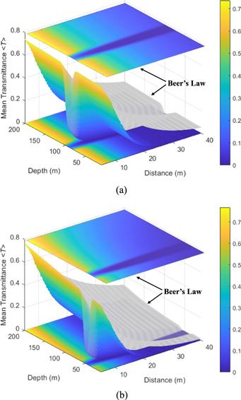
where ${\mathscr{W}}$ is the Lambert function. Moreover, $r=\left({x}_{0},{y}_{0}\right)$ is the beam-centroid vector, $a$ is the receiver telescope radius, and $\varphi $ and $\phi $ are the angle of beam-ellipse orientation and the angle formed by the vector $r$ and the $z$-axis, respectively.For reliable results, the number of Monte Carlo random numerical simulations is set to 10 000. Then, the mean of the PDT on Alice's and Bob's sides can be computed as $\left\langle {T}_{A\left(B\right)}\right\rangle =\displaystyle {\int }_{0}^{{T}_{A\left(B\right)}^{0}}{T}_{A\left(B\right)}P\left({T}_{A\left(B\right)}\right){\rm{d}}{T}_{A\left(B\right)},$ and ${\rm{Var}}(\sqrt{{T}_{A\left(B\right)}})\,=\left\langle {T}_{A\left(B\right)}\right\rangle -{\left\langle \sqrt{{T}_{A\left(B\right)}}\right\rangle }^{2}.$ Figure B2 shows the mean transmittance $\left\langle T\right\rangle $ of oceans S2 and S5 as functions of the depth $d$ and transmission distance $L.$
Figure B2. Mean transmittance as a function of submarine depth and transmission distance, including the effects of extinction and turbulence on ocean S2 for (a) and ocean S5 for (b). Other simulation parameters are set as follows: the dissipation rate of temperature or salinity variance $\zeta ={10}^{-11},$ the kinetic energy dissipation rate $\omega ={10}^{-3},$ the receiver telescope radius $a=0.25{\rm{m}},$ and the initial beam radius ${w}_{0}=80{\rm{mm}}.$ |
Moreover, the grey surface is also plotted for comparison, representing the extinction coefficient transmittance without considering turbulence based on Beer's law in equation (2 ). We observe that the mean transmittance diminishes as horizontal transmission depth increases in both oceans in both seas. However, the mean transmittance is lowest at a depth of 92 m in the S2 ocean, and the different statistics of the S5 ocean result in a depth of 57 m. This finding demonstrates the necessity of varying the depth in terms of ocean type for improved transmission, which we should avoid in the depths of the extinction coefficient peak ranges.
Appendix C. Derivation of the secret key rate
The phase of a coherent state is mapped from the classical binary information and decoded using optical homodyne detection in the QPSK modulation process, as shown in figure 1. The BER ${c}_{{\rm{BER}}}$ of STCQ mentioned encoded by QPSK can be evaluated by the ratio of the carrier power and the noise power when using the CV Bell measurement, which is given by [47]
$\begin{eqnarray}{c}_{{\rm{BER}}}=\displaystyle \frac{1}{2}\text{erfc}\left(\sqrt{\displaystyle \frac{\left(\left\langle {T}_{A}\right\rangle +\left\langle {T}_{B}\right\rangle \right){\eta }_{{\rm{\hom }}}{\alpha }^{2}}{4{\sigma }_{t}{\sigma }_{s}}}\right),\end{eqnarray}$
where $\text{erfc}(\ast )$ is the complementary error function, $\left\langle {T}_{A}\right\rangle $ and $\left\langle {T}_{B}\right\rangle $ are the channel mean transmittance of Alice and Bob, respectively, and ${\eta }_{{\rm{\hom }}}$ denotes the homodyne detection efficiency. Typically, ${\sigma }_{s}=1/4$ is the shot-noise variance when the homodyne detector is shot-noise limited. ${N}_{t}$ stands for the overall noise variance at Charlie's side, which has the form $\begin{eqnarray}\begin{array}{l}{\sigma }_{t}=\left\langle {T}_{A}\right\rangle {\eta }_{{\rm{\hom }}}({\varepsilon }_{tA}+{V}_{{\rm{MA}}})\\ \,+\left\langle {T}_{B}\right\rangle {\eta }_{{\rm{\hom }}}({\varepsilon }_{tB}+{V}_{{\rm{MB}}})+2\left(1+{v}_{{\rm{el}}}\right),\end{array}\end{eqnarray}$
where ${V}_{{\rm{MA}}}$ and ${V}_{{\rm{MB}}}$ are the variance Gaussian modulation for CV-MDI QKD of Alice and Bob, respectively; ${v}_{{\rm{el}}}$ is the electronic noise of the detector, which characterizes all the noises above; and the variance of a vacuum is normalized to 1 [48]. Moreover, the Alice-to-Charlie and Bob-to-Charlie quantum channels incur ${\varepsilon }_{tA}$ and ${\varepsilon }_{tB}$ excess noise, which are defined as $\begin{eqnarray}{\varepsilon }_{tA}={\varepsilon }_{0A}+{\varepsilon }_{\phi },{\varepsilon }_{tB}={\varepsilon }_{0B}+{\varepsilon }_{\phi },\end{eqnarray}$
where ${\varepsilon }_{0A}$ and ${\varepsilon }_{0B}$ are the excess noise of Alice and Bob, which are independent of the amplitude $\alpha $ [49], and ${\varepsilon }_{\phi }={\alpha }^{2}{\sigma }_{\phi }/{\sigma }_{s}$ is the phase noise commonly produced by phase instability in the presence of ${\alpha }^{2}\geqslant \left({V}_{{\rm{MA}}}+1\right){\sigma }_{s}$ [14], where ${\sigma }_{\phi }$ is the extra noise variance.Afterwards, we use the equivalent EB technique and describe the quantum state with a two-mode covariance matrix for easier security analysis. The overall covariance matrix, which is average-weighted by each subchannel at the output of the fluctuating channel, is given by [50]
$\begin{eqnarray}\begin{array}{l}{{\rm{\Sigma }}}_{{\rm{AB}}}=\left(\begin{array}{ll}{\mathscr{A}}{I}_{2} & {\mathscr{C}}{\sigma }_{z}\\ {\mathscr{C}}{\sigma }_{z} & {\mathcal B} {I}_{2}\end{array}\right)\\ =\,\left(\begin{array}{cc}V{I}_{2} & \sqrt{{T}_{{\rm{AB}}}}\sqrt{\left({V}^{2}-1\right)}{\sigma }_{z}\\ \sqrt{{T}_{{\rm{AB}}}}\sqrt{\left({V}^{2}-1\right)}{\sigma }_{z} & {T}_{{\rm{AB}}}\left(V+{\chi }_{t}\right){I}_{2}\end{array}\right),\end{array}\end{eqnarray}$
$\begin{eqnarray}\begin{array}{l}{I}_{2}=\left(\begin{array}{ll}1 & 0\\ 0 & 1\end{array}\right),\,{\sigma }_{z}=\left(\begin{array}{cc}1 & 0\\ 0 & -1\end{array}\right),\,\\ {T}_{{\rm{AB}}}=\displaystyle \frac{\left\langle {T}_{A}\right\rangle }{2}{g}^{2},\sqrt{{T}_{{\rm{AB}}}}=\displaystyle \frac{\left\langle \sqrt{{T}_{A}}\right\rangle }{2}{g}^{2},\end{array}\end{eqnarray}$
where ${T}_{{\rm{AB}}}$ stands for the total quantum channel transmittance between Alice and Bob, for which we can choose the gain of displacement $g=\sqrt{2({V}_{B}-1)}/\left(\sqrt{{T}_{B}}\sqrt{{V}_{B}+1}\right)$ to optimize the equivalent excess noise [17]. $\begin{eqnarray}{\chi }_{{\rm{BE}}}=\displaystyle \sum _{i=1}^{2}G\left(\displaystyle \frac{{\lambda }_{i}-1}{2}\right)-\displaystyle \sum _{i=3}^{3}G\left(\displaystyle \frac{{\lambda }_{i}-1}{2}\right),\end{eqnarray}$
where the required symplectic eigenvalues of ${{\rm{\Sigma }}}_{{\rm{AB}}}$ have the form $\begin{eqnarray}{\lambda }_{1,2}^{2}=\displaystyle \frac{1}{2}\left({\rm{\Delta }}\pm \sqrt{{{\rm{\Delta }}}^{2}-4{D}^{2}}\right),\end{eqnarray}$
where ${\rm{\Delta }}={{\mathscr{A}}}^{2}+{ {\mathcal B} }^{2}-2{{\mathscr{C}}}^{2},$ $D={\mathscr{A}} {\mathcal B} -{{\mathscr{C}}}^{2},$ and ${\lambda }_{3}={\mathscr{A}}-{{\mathscr{C}}}^{2}/\left( {\mathcal B} +1\right).$ Without losing generality, we assume that the variances obey $V={V}_{A}={V}_{B}={V}_{{\rm{MA}}}+1={V}_{{\rm{MB}}}+1,$ and the secret key is generated using both the $x$ and $p$ quadrature components. Furthermore, between Alice's and Bob's heterodyne measurements, the Shannonian mutual information is provided by $\begin{eqnarray}\begin{array}{l}{I}_{{\rm{AB}}}=2\times \displaystyle \frac{1}{2}{\mathrm{log}}_{2}\left(\displaystyle \frac{{\mathscr{A}}+1}{{\mathscr{A}}+1-{{\mathscr{C}}}^{2}/\left( {\mathcal B} +1\right)}\right)\\ =\,{\mathrm{log}}_{2}\left[\displaystyle \frac{{T}_{{\rm{AB}}}{V}_{{\rm{MA}}}+1+{T}_{{\rm{AB}}}\left(1+{\chi }_{t}\right)}{1+{T}_{{\rm{AB}}}\left(1+{\chi }_{t}\right)}\right].\end{array}\end{eqnarray}$
Moreover, the total amount of detection-induced noise and equivalent excess noise is denoted by ${\chi }_{t},$ which has the form
$\begin{eqnarray}{\chi }_{t}=\displaystyle \frac{1}{{T}_{{\rm{AB}}}}-1+\varepsilon ^{\prime} +\displaystyle \frac{2{\chi }_{{\rm{\hom }}}}{\left\langle {T}_{A}\right\rangle },\end{eqnarray}$
where ${\chi }_{{\rm{\hom }}}$ is the detection noise related to the electronic noise variance ${v}_{{\rm{el}}}$ and the detection efficiency ${\eta }_{{\rm{\hom }}},$ which is given by $\begin{eqnarray}{\chi }_{{\rm{\hom }}}=\displaystyle \frac{{v}_{{\rm{el}}}}{{\eta }_{{\rm{\hom }}}}+\displaystyle \frac{1-{\eta }_{{\rm{\hom }}}}{{\eta }_{{\rm{\hom }}}},\end{eqnarray}$
and $\varepsilon ^{\prime} $ is the equivalent excess noise, which is given by $\begin{eqnarray}\begin{array}{l}\varepsilon ^{\prime} ={\varepsilon }_{tA}+\displaystyle \frac{2}{\left\langle {T}_{A}\right\rangle }+\displaystyle \frac{{\alpha }^{2}}{{\sigma }_{s}}{c}_{{\rm{BER}}}\\ \,+\displaystyle \frac{\left\langle {T}_{B}\right\rangle }{\left\langle {T}_{A}\right\rangle }\left({\varepsilon }_{tB}-2+\displaystyle \frac{{\alpha }^{2}}{{\sigma }_{s}}{c}_{{\rm{BER}}}\right)-\displaystyle \frac{{N}_{E}}{\left\langle {T}_{A}\right\rangle },\end{array}\end{eqnarray}$
where the noise contribution caused by Eve's two-mode correlation is ${N}_{E},$ which can be calculated by the correlation components of Eve's $x$ quadrature or $p$ quadrature as $\begin{eqnarray}\begin{array}{l}{N}_{E}=\displaystyle \frac{2}{\left\langle {T}_{A}\right\rangle }\sqrt{\left(1-\left\langle {T}_{A}\right\rangle \right)\left(1-\left\langle {T}_{B}\right\rangle \right)}\left\langle {E}_{{1}_{X}}{E}_{{2}_{X}}\right\rangle \\ \,=-\displaystyle \frac{2}{\left\langle {T}_{A}\right\rangle }\sqrt{\left(1-\left\langle {T}_{A}\right\rangle \right)\left(1-\left\langle {T}_{B}\right\rangle \right)}\left\langle {E}_{{1}_{P}}{E}_{{2}_{P}}\right\rangle ,\end{array}\end{eqnarray}$
where $\begin{eqnarray}\begin{array}{l}\left\langle {E}_{{1}_{X}}{E}_{{2}_{X}}\right\rangle =-\left\langle {E}_{{1}_{P}}{E}_{{2}_{P}}\right\rangle =-\sqrt{{V}_{E}^{2}-1}\\ \,=-\sqrt{{\left(1+\displaystyle \frac{\left\langle {T}_{A}\right\rangle }{1-\left\langle {T}_{A}\right\rangle }{\varepsilon }_{tA}\right)}^{2}-1},\end{array}\end{eqnarray}$
representing the modes of Charlie's side under the correlated attacks by Eve [51]. We estimate the SKR above under the premise of the two-mode attack because the two-mode attack is shown to be the most effective [26], so Eve uses a two-mode correlated coherent Gaussian attack, introducing quantum correlations $\left\{{\rm{E1}},{\rm{E2}}\right\}$ in both quantum channels. Moreover, Eve stores the ancillary states interacted with Alice and Bob to the quantum memory (QM), then deduces the secret key by executing an optimum collective measurement on the ensemble of stored ancilla anytime.It is worth noting that the two-mode attack may degenerate into a one-mode attack when the correlation between the two quantum channels becomes weak, in which Eve uses her half of each EPR pair to conduct entangling cloning on Alice's and Bob's modes individually [52]. Furthermore, these two forms of assault are similar in the extremely asymmetric situation, where Bob is physically adjacent to Charlie. Conversely, the double-mode attack on the key rate will be more formidable when Alice and Bob are more symmetric with respect to Eve. As indicated in equation (C12 ), the correlation between Eve's two modes will decrease sharply and degenerate into a one-mode attack when extreme asymmetry occurs, namely ${L}_{{\rm{BC}}}\approx 0,\left\langle {T}_{{\rm{BC}}}\right\rangle \approx 1.$
Additionally, we further consider the finite-size effect, and the most important parameter in equation (8) is related to the security of the private key amplification [53], which is given by
$\begin{eqnarray}{\rm{\Delta }}(n)=\left(2\dim { {\mathcal H} }_{X}+3\right)\sqrt{\displaystyle \frac{{\mathrm{log}}_{2}(2/\bar{\epsilon })}{n}}+\displaystyle \frac{2}{n}{\mathrm{log}}_{2}\left(1/{\epsilon }_{{\rm{PF}}}\right),\end{eqnarray}$
where ${ {\mathcal H} }_{X}$ is the dimension of the Hilbert space corresponding to the variable x used in the raw key, which takes $\dim { {\mathcal H} }_{X}=2$ in our STCQ protocol encoded by the binary bits. Moreover, $\bar{\epsilon }$ is a smoothing parameter, and ${\epsilon }_{{\rm{PF}}}$ is the failure probability of the privacy amplification procedure.In this finite-size scenario, the estimation of the covariance matrix ${{\rm{\Sigma }}}_{{\epsilon }_{{\rm{PA}}}}$ is made through the sampling of $\left( {\mathcal M} -{\mathscr{N}}\right)$ couples of correlated variables ${\left({{\mathscr{X}}}_{i},{{\mathscr{Y}}}_{i}\right)}_{i=1\cdots m},$ and the data between Alice and Bob are linked through the correlated linear relation, which has the form
$\begin{eqnarray}{\mathscr{Y}}=t{\mathscr{X}}+{\mathscr{Z}},\end{eqnarray}$
where $t=\sqrt{\left\langle T\right\rangle }$ and ${\mathscr{Z}}$ follows a centered normal distribution with unknown variance ${\sigma }^{2}=1+\left\langle T\right\rangle \xi .$ We can minimize the SKR with a probability of at least $1-{\epsilon }_{{\rm{PA}}}$ once we find the covariance matrix, which is given as $\begin{eqnarray}{{\rm{\Sigma }}}_{{\epsilon }_{{\rm{PF}}}}=\left(\begin{array}{ll}\left({V}_{B}+1\right){I}_{2} & {t}_{\min }\sqrt{\left({V}^{2}-1\right)}{\sigma }_{z}\\ {t}_{\min }\sqrt{\left({V}^{2}-1\right)}{\sigma }_{z} & \left({{t}_{\min }}^{2}{V}_{B}+{{\sigma }_{\max }}^{2}\right){I}_{2}\end{array}\right),\end{eqnarray}$
where ${t}_{\min }$ represents the minimal value of $t,$ and ${\sigma }_{\max }$ is the maximal value of $\sigma ,$ which is compatible with sampled couples except with probability ${\epsilon }_{{\rm{PF}}}/2.$ Here, the maximum-likelihood estimators are used for the normal linear model $\begin{eqnarray}\hat{t}=\displaystyle \sum _{i=1}^{m}{x}_{i}{y}_{i}/\displaystyle \sum _{i=1}^{m}{x}_{i}^{2},\,{\hat{\sigma }}^{2}=\displaystyle \frac{1}{m}\displaystyle \sum _{i=1}^{m}{\left({y}_{i}-\hat{t}{x}_{i}\right)}^{2}.\end{eqnarray}$
Using the expected values of $E[\hat{t}]=\sqrt{\left\langle T\right\rangle }$ and $E\left[{\hat{\sigma }}^{2}\right]\,=1+\left\langle T\right\rangle {\zeta }_{t}$ for analysing the protocol from a theoretical point of view, the computed results are given as
$\begin{eqnarray}\begin{array}{l}{t}_{\min }\approx \sqrt{\left\langle T\right\rangle }-{{\mathscr{Z}}}_{{\epsilon }_{{\rm{PF}}}/2}\sqrt{\displaystyle \frac{1+\left\langle T\right\rangle \hat{\xi }}{\left( {\mathcal M} -{\mathscr{N}}\right){V}_{A}}},\\ {{\sigma }_{\max }}^{2}\approx 1+\left\langle T\right\rangle \xi +{{\mathscr{Z}}}_{{\epsilon }_{{\rm{PF}}}/2}\displaystyle \frac{\sqrt{2}(1+\left\langle T\right\rangle \xi )}{\sqrt{\left( {\mathcal M} -{\mathscr{N}}\right)}},\end{array}\end{eqnarray}$
where ${{\mathscr{Z}}}_{{\epsilon }_{{\rm{PF}}}/2}=1-\text{erf}\left({z}_{{\epsilon }_{{\rm{PF}}}/2}/\sqrt{2}\right)/2={\epsilon }_{{\rm{PF}}}/2,$ and the optimal value for the error probabilities can be set to $\bar{\epsilon }={\epsilon }_{{\rm{PF}}}={10}^{-10}.$