


1. Introduction
Quantum metrology is of importance for multiple areas of scientific research, including gravitational wave detection [1, 2], biological sensing [3, 4], atomic clocks [5, 6], and so on. One of the main tasks of quantum metrology can be attributed to a phase estimation problem, where the estimation precision of an unknown phase shift θ depends on the probes, the phase accumulation, and the measurement scheme [7–14]. For instance, performing the intensity measurements at the output ports of a coherent-state light interferometer, the output signal $\propto {\sin }^{2}(\theta /2)$ or ${\cos }^{2}(\theta /2)$, where θ is an unknown phase shift. The signal exhibits the full width at half maximum (FWHM) = π, corresponding to the Rayleigh resolution limit [15]. On the other hand, the achievable phase sensitivity is subject to the shot-noise limit (SNL) $1/\sqrt{\bar{n}}$ [16, 17], where $\bar{n}$ is the mean number of photons injected into the interferometer.
To beat the above classical limits, one can use nonclassical resources such as squeezed state [18–21] and N-photon entangled state [22–28]. In 1981, Caves [18] proposed a squeezed-state interferometer, where a coherent state and a squeezed vacuum state are injected into the two input ports, as depicted by figure 1(a). It has been shown that the achievable sensitivity can beat the SNL. Furthermore, the so-called Heisenberg-limit (HL) can be reached by using the N-photon entangled states [23–25], or squeezed states [19–21]. However, the entangled states are difficult to prepare and are extremely fragile. On the other hand, the measurement schemes based on a coherent state and a squeezed vacuum state [19–21] with coincidence photon counting or parity detection are not highly efficient and are dependent on the number resolvable counters. Indeed, the achievable sensitivity is subject to the finite number resolution of the photon counters [29, 30]. Recently, Schäfermeier et al [31] have realized deterministic super-resolution and super-sensitivity simultaneously in the squeezed-state interferometer with a single-port homodyne detection, where the measurement data is divided into p1 ∈ [−a, a] and p1 ∉ [−a, a], where a is a parameter that can be adjusted artificially. This is equivalent to a binary-outcome measurement.
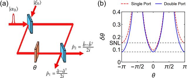
Figure 1. (a) Homodyne detection (i.e. measuring the quadrature operators ${\hat{p}}_{1}$ and ${\hat{p}}_{2}$) at two ports of the interferometer that is fed by a coherent state ∣α0⟩ and a squeezed vacuum ∣ξ0⟩. (b) The achievable phase sensitivity for the double-port homodyne detection (blue solid line), is better than that of the single-port homodyne detection (red dashed line). Vertical lines in (b): the SNL $1/\sqrt{\bar{n}}$ and the best sensitivity $1/\sqrt{(1+{{\rm{e}}}^{2r}){\bar{n}}_{a}}$. The parameters: ${\bar{n}}_{a}=42$, e−r = 0.6 and ϱ = 0.5. |
Obviously, the above single-port homodyne detection neglects almost half of the total phase information at another output port, leading to a reduced phase estimation precision. In this paper, we propose a double-port homodyne detection scheme with proper data processing. Specifically, we divide the two-dimensional measurement quadrature (p1, p2) into two regions, which realize a similar binary-outcome measurement with that of Schäfermeier et al [31]. We calculate the full width at half maximum (FWHM) of the output signal and the phase estimation precision using the inversion estimator. Our results show that a 1.8-fold improvement in the sensitivity and a 30-fold improvement in the resolution beyond their associated classical limits can be realized with about 400 input photons, which is slightly better than that of [31]. Finally, it should be mentioned that there are many kinds of data processing in the two-dimensional measurement quadrature (p1, p2). Here we show the simplest one to realize a further improvement in the resolution and in the sensitivity beyond that of [31].
2. Double-port homodyne detection without data processing
As illustrated by figure 1(a), we consider the two-port homodyne detection in the squeezed-state interferometer, equivalently measuring the field quadratures ${\hat{p}}_{1}\,=(\hat{a}-{\hat{a}}^{\dagger })/(2{\rm{i}})$ and ${\hat{p}}_{2}=(\hat{b}-{\hat{b}}^{\dagger })/(2{\rm{i}})$. In order to maximize the quantum Fisher information (see the appendix ), we choose a coherent state and a squeezed vacuum state with real field amplitudes [18, 19, 29, 30], corresponding to the input state ∣$Psi$in⟩ = ∣α0⟩ ⨂ ∣ξ0⟩, with ${\alpha }_{0}=\sqrt{{\bar{n}}_{a}}\in {\mathbb{R}}$ and ${\xi }_{0}=-r\in {\mathbb{R}}$. The average photon number of the input state is given by $\bar{n}={\bar{n}}_{a}+{\bar{n}}_{b}$, where ${\bar{n}}_{a}={\alpha }_{0}^{2}$ is the average photon number of coherent state and ${\bar{n}}_{b}={\sinh }^{2}r$ is the average photon number of the squeezed vacuum state.
The Wigner function of the input state is given by [32]9 ) becomes ${F}_{\max }\approx {\bar{n}}^{2}$, which leads to a Heisenberg scaling precision $\delta {\theta }_{\min }\approx 1/\bar{n}$.
$\begin{eqnarray}\begin{array}{l}{W}_{\mathrm{in}}(\alpha ,\beta )=\displaystyle \frac{2}{\pi }{{\rm{e}}}^{-2\left[{\left({x}_{1}-{\alpha }_{0}\right)}^{2}+{p}_{1}^{2}\right]}\\ \quad \times \displaystyle \frac{2}{\pi }\sqrt{\tilde{\mu }\tilde{\nu }}{{\rm{e}}}^{-2\left(\tilde{\mu }{x}_{2}^{2}+\tilde{\nu }{p}_{2}^{2}\right)},\end{array}\end{eqnarray}$
with the parameters $\tilde{\mu }$ and $\tilde{\nu }$ dependent on the input state, and the variables α = x1 + ip1 and β = x2 + ip2. Here, the subscripts “1” and “2” denote two different paths (or the field modes) a and b. Following Schäfermeier et al [31], we consider the squeezed vacuum with the purity ϱ < 1 and take $\tilde{\mu }={\varrho }^{2}{{\rm{e}}}^{-2r}$ and $\tilde{\nu }={{\rm{e}}}^{2r}$, where e−r describes the squeeze factor of ∣ξ0⟩. The phase accumulation can be described by the unitary operator: $\begin{eqnarray}\hat{U}(\theta )={{\rm{e}}}^{-{\rm{i}}\pi {\hat{J}}_{y}/2}{{\rm{e}}}^{-{\rm{i}}\theta {\hat{a}}^{\dagger }\hat{a}}{{\rm{e}}}^{-{\rm{i}}\pi {\hat{J}}_{y}/2},\end{eqnarray}$
where $\exp (-{\rm{i}}\pi {\hat{J}}_{y}/2)$ and $\exp (-{\rm{i}}\theta {\hat{a}}^{\dagger }\hat{a})$ represent the actions of the 50:50 beam splitter and that of the phase accumulation in the path, with ${\hat{J}}_{y}=({\hat{a}}^{\dagger }\hat{b}-{\hat{b}}^{\dagger }\hat{a})/2{\rm{i}}$ and $\hat{a}$, $\hat{b}$ being bosonic annihilation operators. The Wigner function of the output state $| {\psi }_{\mathrm{out}}\rangle =\hat{U}(\theta )| {\psi }_{\mathrm{in}}\rangle $ takes the same form as that of the input state, i.e. ${W}_{\mathrm{out}}(\alpha ,\beta )={W}_{\mathrm{in}}({\tilde{\alpha }}_{\theta },{\tilde{\beta }}_{\theta })$, with $\begin{eqnarray}\left\{\begin{array}{l}{\tilde{\alpha }}_{\theta }=\alpha \displaystyle \frac{{{\rm{e}}}^{{\rm{i}}\theta }-1}{2}+\beta \displaystyle \frac{{{\rm{e}}}^{{\rm{i}}\theta }+1}{2},\\ {\tilde{\beta }}_{\theta }=-\alpha \displaystyle \frac{{{\rm{e}}}^{{\rm{i}}\theta }+1}{2}-\beta \displaystyle \frac{{{\rm{e}}}^{{\rm{i}}\theta }-1}{2}.\end{array}\right.\end{eqnarray}$
Integrating Wout(α, β) over x1 and x2, we obtain the conditional probability for detecting a measurement outcome: $\begin{eqnarray}\begin{array}{l}P({p}_{1},{p}_{2}| \theta )\\ \quad =\displaystyle \frac{2}{\pi }\sqrt{\displaystyle \frac{1}{\varepsilon }}{{\rm{e}}}^{-\tfrac{1}{\varepsilon }\left(2{\eta }_{+}{p}_{1}^{2}+2{\eta }_{-}{p}_{2}^{2}+\tfrac{\tilde{\mu }-\tilde{\nu }}{\tilde{\mu }\tilde{\nu }}{\sin }^{2}\theta {p}_{1}{p}_{2}+\displaystyle \frac{{\alpha }^{2}}{2}\displaystyle \frac{1+\tilde{\nu }}{\tilde{\nu }}{\sin }^{2}\theta \right)}\\ \quad \times \,{{\rm{e}}}^{-\tfrac{\alpha \sin \theta }{\varepsilon \tilde{\nu }}\left[(\tilde{\nu }+1)({p}_{1}+{p}_{2})+(\tilde{\nu }-1)\cos \theta ({p}_{1}-{p}_{2})\right]},\end{array}\end{eqnarray}$
where we introduced $\begin{eqnarray}\varepsilon =\displaystyle \frac{4\tilde{\mu }+(\tilde{\mu }\tilde{\nu }+\tilde{\nu }-3\tilde{\mu }+1){\sin }^{2}\theta }{4\tilde{\mu }\tilde{\nu }},\end{eqnarray}$
and $\begin{eqnarray}{\eta }_{\pm }=\displaystyle \frac{\tilde{\mu }+\tilde{\nu }+2\tilde{\mu }\tilde{\nu }\pm 2\tilde{\mu }(\tilde{\nu }-1)\cos \theta +(\tilde{\mu }-\tilde{\nu }){\cos }^{2}\theta }{4\tilde{\mu }\tilde{\nu }}.\end{eqnarray}$
The achievable phase sensitivity is given by $\begin{eqnarray}\delta \theta =1/\sqrt{F(\theta )},\end{eqnarray}$
where F(θ) is the classical Fisher information (CFI): $\begin{eqnarray}\begin{array}{rcl}F(\theta ) & = & {\displaystyle \int }_{-\infty }^{\infty }{\displaystyle \int }_{-\infty }^{\infty }{\rm{d}}{p}_{1}{\rm{d}}{p}_{2}P({p}_{1},{p}_{2}| \theta )\\ & & \times {\left[\displaystyle \frac{\partial \mathrm{ln}P({p}_{1},{p}_{2}| \theta )}{\partial \theta }\right]}^{2}.\end{array}\end{eqnarray}$
In figure 1(b), we show the achievable phase sensitivity of double-port homodyne detection (blue solid line) as a function of the phase θ. One can find that the phase sensitivity can beat SNL around the optimal phase point θ = 0, ±π, which gives the maximal CFI $\begin{eqnarray}{F}_{\max }=({{\rm{e}}}^{2r}+1){\bar{n}}_{a},\end{eqnarray}$
and the best sensitivity $\begin{eqnarray}\delta {\theta }_{\min }=1/\sqrt{({{\rm{e}}}^{2r}+1){\bar{n}}_{a}}.\end{eqnarray}$
When the squeeze factor r = 0 (i.e. ${\bar{n}}_{b}=0$), we have ${F}_{\max }=2{\bar{n}}_{a}=2\bar{n}$ and $\delta {\theta }_{\min }=1/\sqrt{2\bar{n}}$. To attain a better sensitivity, we can take the squeeze factor r > 0 (i.e. ${\bar{n}}_{b}\gt 0$). Especially, for the case of ${\bar{n}}_{b}={\bar{n}}_{a}=\bar{n}/2\gg 1$, we have the relation ${\bar{n}}_{b}={\sinh }^{2}r\approx {{\rm{e}}}^{2r}/4$. Therefore, equation (3. Single-port homodyne detection without data processing
If we do not take into account the quadrature p2, the scheme is reduced to the single-port homodyne detection, as demonstrated in [31]. Integrating P(p1, p2∣θ) over p2, we can obtain the conditional probability of the single-port homodyne detection, i.e.13 ) and taking θ = 0, we obtain the maximal CFI
$\begin{eqnarray}P({p}_{1}| \theta )=\sqrt{\displaystyle \frac{2}{\pi {\eta }_{-}}}\exp \left[-\displaystyle \frac{2}{{\eta }_{-}}{\left({p}_{1}+\displaystyle \frac{{\alpha }_{0}}{2}\sin \theta \right)}^{2}\right].\end{eqnarray}$
With the single-port homodyne detection, one can easily obtain the output signal $\begin{eqnarray}\langle {\hat{p}}_{1}(\theta )\rangle ={\int }_{-\infty }^{\infty }{p}_{1}P({p}_{1}| \theta ){\rm{d}}{p}_{1}=-\displaystyle \frac{{\alpha }_{0}}{2}\sin \theta ,\end{eqnarray}$
which exhibits FWHM = 2π/3, and hence the Rayleigh limit in fringe resolution [31, 33]. On the other hand, the achievable CFI reads [34]: $\begin{eqnarray}\begin{array}{rcl}{F}_{s}(\theta ) & = & {\displaystyle \int }_{-\infty }^{\infty }\displaystyle \frac{{[\partial P({p}_{1}| \theta )/\partial \theta ]}^{2}}{P({p}_{1}| \theta )}{\rm{d}}{p}_{1}\\ & = & \displaystyle \frac{{\left({\alpha }_{0}\cos \theta \right)}^{2}}{{\eta }_{-}}+\displaystyle \frac{{[\tilde{\mu }-\tilde{\mu }\tilde{\nu }+(\tilde{\mu }-\tilde{v})\cos \theta ]}^{2}{\sin }^{2}\theta }{8{\left(\tilde{\mu }\tilde{\nu }{\eta }_{-}\right)}^{2}},\end{array}\end{eqnarray}$
and hence the achievable sensitivity $\begin{eqnarray}\delta {\theta }_{s}=1/\sqrt{{F}_{s}(\theta )}.\end{eqnarray}$
When the coherent-state component dominates over the squeezed vacuum (i.e. ${\bar{n}}_{a}\gg {\bar{n}}_{b}$), the best sensitivity occurs at the optimal working point θ = 0. Using equation ( $\begin{eqnarray}{F}_{s,\max }(0)={{\rm{e}}}^{2r}{\bar{n}}_{a},\end{eqnarray}$
and hence the best sensitivity approximates to ${{\rm{e}}}^{-r}/\sqrt{\bar{n}}$ [34], which is in agreement with the light intensity-difference measurement as ${\bar{n}}_{a}\gg {\bar{n}}_{b}$ [18, 19]. When the squeeze factor r = 0, the phase sensitivity is limited to the SNL, as shown in [32, 33]. To beat the SNL, it is necessary to take the squeeze factor r > 0.Comparing equations (9 ) and (15 ), the maximal CFI of double-port homodyne detection is greater than that of the single-port homodyne detection, which means that we can attain a better phase sensitivity by the double-port homodyne detection. This is because, the single-port homodyne detection only takes into account the contribution of p1, which lost some information of the unknown phase θ. In figure 1(b), we show the difference in achievable phase sensitivity between single-port homodyne detection and double-port homodyne detection. One can find that the double-port homodyne detection is better than the single-port homodyne detection in the whole phase interval θ ∈ [−π, π], and can beat the SNL around θ = 0, ±π. In order to improve the resolution determined by the FWHM, we can adopt suitable data processing over the measurement outcomes. In the next section, we will discuss binary-outcome measurement data processing.
4. Binary-outcome homodyne detection
The phase resolution can be improved by suitable data processing over the measurement outcomes, at the cost of reduced phase sensitivity. For the case of the single-port homodyne detection, Schäfermeier et al [31] have demonstrated super-sensitive and super-resolving phase measurement in the squeezed-state interferometer. The data-processing method they adopted is to separate the measurement quadrature p1 ∈ (−∞, ∞) into two bins: p1 ∈ [−a, a] and p1 ∉ [−a, a] (shown in figure 2 (c)), where a is a controllable parameter. This is equivalent to a binary-outcome measurement [35, 36], with the observable $\hat{{\rm{\Pi }}}={\mu }_{0}{\hat{{\rm{\Pi }}}}_{0}+{\mu }_{\varnothing }{\hat{{\rm{\Pi }}}}_{\varnothing }$, where μ0 and ${\mu }_{\varnothing }$ are arbitrary numbers. Furthermore, the projection operators are given by ${\hat{{\rm{\Pi }}}}_{0}={\int }_{-a}^{a}| {p}_{1}\rangle \langle {p}_{1}| {\rm{d}}{p}_{1}$, and ${\hat{{\rm{\Pi }}}}_{\varnothing }=1-{\hat{{\rm{\Pi }}}}_{0}$. Using the relation ${P}_{k}(\theta )=\langle {\psi }_{\mathrm{out}}| {\hat{{\rm{\Pi }}}}_{k}| {\psi }_{\mathrm{out}}\rangle $, we obtain the probabilities of each outcome:6 ). With such a kind of binary-outcome measurement, one can construct the output signal
$\begin{eqnarray}{P}_{0}(\theta )={\int }_{-a}^{a}{\rm{d}}{p}_{1}P({p}_{1}| \theta )=\displaystyle \frac{1}{2}\mathrm{Erf}\left[{g}_{-}(\theta ),{g}_{+}(\theta )\right],\end{eqnarray}$
$\begin{eqnarray}{P}_{\varnothing }(\theta )=1-{P}_{0}(\theta ),\end{eqnarray}$
where $\mathrm{Erf}\left[x,y\right]\equiv \mathrm{erf}[y]-\mathrm{erf}[x]$ denotes a generalized error function, and $\begin{eqnarray}{g}_{\pm }(\theta )=\sqrt{\displaystyle \frac{2}{{\eta }_{-}}}\left(\displaystyle \frac{{\alpha }_{0}}{2}\sin \theta \pm a\right),\end{eqnarray}$
with η− being defined by equation ( $\begin{eqnarray}\langle \hat{{\rm{\Pi }}}(\theta )\rangle ={\mu }_{0}{P}_{0}(\theta )+{\mu }_{\varnothing }{P}_{\varnothing }(\theta ),\end{eqnarray}$
where μ0 and ${\mu }_{\varnothing }$ are arbitrary numbers. Similar to Schäfermeier et al [31], we take ${\mu }_{\varnothing }=0$, and ${\mu }_{0}=1/\mathrm{erf}(\sqrt{2\tilde{\nu }}a)$. To estimate an unknown phase shift θ0, we solve the equation $\begin{eqnarray}\langle \hat{{\rm{\Pi }}}(\theta )\rangle ={\mu }_{0}{P}_{0}(\theta )\approx {\mu }_{0}\displaystyle \frac{{{ \mathcal N }}_{0}}{{ \mathcal N }},\end{eqnarray}$
which gives the inversion estimator θinv, where ${{ \mathcal N }}_{0}$ denotes the occurrence number of the outcome “0” in ${ \mathcal N }$ independent measurements. Repeating the above process M times, we obtain M estimators $\{{\theta }_{\mathrm{inv}}^{(1)},{\theta }_{\mathrm{inv}}^{(2)},\cdots ,{\theta }_{\mathrm{inv}}^{(M)}\}$, which give the statistical average and the root mean square error $\begin{eqnarray}\sigma =\sqrt{\sum _{i=1}^{M}\displaystyle \frac{{({\theta }_{\mathrm{inv}}^{(i)}-{\theta }_{0})}^{2}}{M}},\end{eqnarray}$
which can quantify the performance of the estimator θinv. According to the error-propagation formula [37], the phase sensitivity is $\begin{eqnarray}\delta {\theta }_{\mathrm{bin}}=\displaystyle \frac{{\rm{\Delta }}\hat{{\rm{\Pi }}}}{\left|\partial \langle \hat{{\rm{\Pi }}}(\theta )\rangle /\partial \theta \right|}=\displaystyle \frac{\sqrt{{P}_{0}(\theta )(1-{P}_{0}(\theta ))}}{\left|\tfrac{\partial {P}_{0}(\theta )}{\partial \theta }\right|},\end{eqnarray}$
where ${\rm{\Delta }}\hat{{\rm{\Pi }}}=\sqrt{\langle {\hat{{\rm{\Pi }}}}^{2}\rangle -\langle \hat{{\rm{\Pi }}}{\rangle }^{2}}$ denotes the root-mean-square fluctuation of the signal. When the repeat time M → ∞, the sensitivity δθbin can be saturated by $\sqrt{{ \mathcal N }}\sigma $.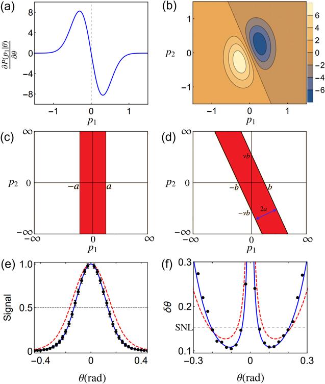
Figure 2. (a) ∂P(p1∣θ)/∂θ as a function of the quadrature p1. (b) Density plot of ∂P(p1, p2∣θ)/∂θ as a function of the quadratures p1 and p2, where we take θ = 0. (c) and (d) The data processing schemes of binary-outcome measurement corresponding to single-port homodyne detection (c) and double-port homodyne detection (d), where the region width of the two schemes are 2a. (e) and (f) The output signal and the sensitivity of the binary-outcome measurement with single-port homodyne detection (red dashed lines) and double-port homodyne detection (blue lines). The black circles are simulated by M = 500 repeats of ${ \mathcal N }=300$ independent measurements. Parameters: ${\bar{n}}_{a}=42$, e−r = 0.47, a = 0.5, $b=\sqrt{1+{{\rm{e}}}^{-4r}}a=0.512$ and ϱ = 0.5. |
Next, we consider the double-port homodyne detection with a binary-outcome measurement data processing, i.e. separate the measurement quadrature p1 and p2 into two regions. The data processing method we use is inspired by figure 2(b), in which we show the density plot of ∂P(p1, p2∣θ)/∂θ as a function of the measurement quadratures p1 and p2 with θ = 0. One can find that it is symmetric with respect to the line ${p}_{2}+\tilde{\nu }{p}_{1}=0$, which inspires us to treat the region $-\tilde{\nu }({p}_{1}+b)\lt {p}_{2}\lt -\tilde{\nu }({p}_{1}-b)$ as an outcome ‘0' and other regions as an outcome ‘$\varnothing $' (shown in figure 2(d)), where19 ). In figure 2(c), we show the output signals with the parameter a = 0.5. The resolution is determined by the FWHM of the signal. One can find that the blue line (double-port detection) shows a better phase resolution than that of the single-port detection adopted by Schäfermeier et al [31].
$\begin{eqnarray}b=\sqrt{1+1/{\tilde{\nu }}^{2}}a=\sqrt{1+{{\rm{e}}}^{-4r}}a,\end{eqnarray}$
and the region width 2a is a controllable parameter. The corresponding conditional probabilities are: $\begin{eqnarray}\begin{array}{rcl}\tilde{{P}_{0}}(\theta ) & = & {\displaystyle \int }_{-\infty }^{\infty }{\rm{d}}{p}_{1}{\displaystyle \int }_{-\tilde{\nu }({p}_{1}+b)}^{-\tilde{\nu }({p}_{1}-b)}{\rm{d}}{p}_{2}P({p}_{1},{p}_{2}| \theta )\\ & = & \displaystyle \frac{1}{2}\mathrm{Erf}\left[{h}_{-}(\theta ),{h}_{+}(\theta )\right],\end{array}\end{eqnarray}$
$\begin{eqnarray}\tilde{{P}_{\varnothing }}(\theta )=1-\tilde{{P}_{0}}(\theta ),\end{eqnarray}$
where $\begin{eqnarray}\begin{array}{rcl}{h}_{\pm }(\theta ) & = & \sqrt{\displaystyle \frac{2}{(1+\tilde{\nu })({\eta }_{+}+\tilde{\nu }{\eta }_{-}-1)}}\\ & & \times \left[\displaystyle \frac{{\alpha }_{0}}{2}(1+\tilde{\nu })\sin \theta \pm \tilde{\nu }b\right].\end{array}\end{eqnarray}$
We construct the output signal by taking ${\mu }_{\varnothing }=0$, ${\mu }_{0}=1/\mathrm{erf}(\sqrt{2(1+{\tilde{\nu }}^{2})/(1+\tilde{\nu })}a)$ and replacing P0(θ) by $\tilde{{P}_{0}}(\theta )$ in equation (The phase sensitivity can be also given by equation (22 ) with P0(θ) replaced by $\tilde{{P}_{0}}(\theta )$. In figure 2(e), we show the phase sensitivity with parameter a = 0.5, which is almost saturated by $\sqrt{{ \mathcal N }}\sigma $, where σ is simulated by M = 500 repeats of ${ \mathcal N }=300$ independent measurements. For the double-port detection (the blue line), the achievable sensitivity $\delta {\theta }_{\min \ }$ appears at the optimal point ${\theta }_{\min }=0.11$ and is better than the single-port detection (red dashed line).
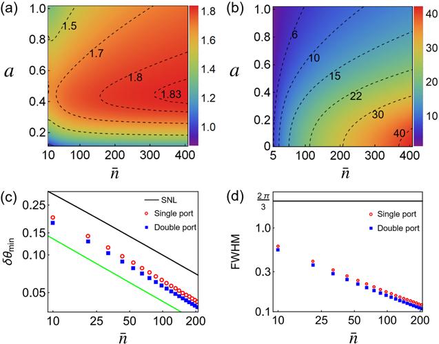
The value of a is a trade-off parameter that controls the achievable sensitivity and the resolution. In figures 3(a) and (b), we show a density plot of the ratios $\tfrac{1/\sqrt{\bar{n}}}{\delta {\theta }_{\min \ }}$ and $\tfrac{2\pi /3}{\mathrm{FWHM}}$ as functions of the average photon number $\bar{n}$ and the parameter a, where $\delta {\theta }_{\min \ }$ is the best sensitivity. Using the parameters similar to Schäfermeier et al [31], one can find that the resolution is optimal as a → 0, while the best sensitivity appears at a ∼ 0.42. When the average photon number $\bar{n}\sim 400$ and the parameter a ∼ 0.4, we can obtain a 1.8-fold improvement in the sensitivity and a 30-fold improvement in the resolution, which is better than the experimental result in [31], where a 1.7-fold improvement in the sensitivity and a 22-fold improvement in the resolution with $\bar{n}=430$ has been demonstrated. In figures 3(c) and (d), we show the log–log plot of the best sensitivity $\delta {\theta }_{\min }$ and the FWHM against the photon number $\bar{n}$. One can find that both the best sensitivity and the FWHM of the double-port detection are better than that of the single-port detection.
Figure 3. (a) and (b) Density plots of the ratios $\tfrac{1/\sqrt{\bar{n}}}{\delta {\theta }_{\min }}$ and $\tfrac{2\pi /3}{\mathrm{FWHM}}$ as functions of the average photon number $\bar{n}$ and the parameter a, with the parameters e−r = 0.47 and ϱ = 0.5 [31]. (c) and (d) Log–log plot of the achievable sensitivity $\delta {\theta }_{\min }$ and the FWHM against the photon number $\bar{n}$. The green solid line in (c) is given by equation ( |
5. Conclusion
In summary, we have proposed a double-port homodyne detection in the interferometer with proper data processing, where the input states are the coherent state and squeezed vacuum state. Performing the double-port homodyne detection without any data processing, we show that the best sensitivity is $\delta {\theta }_{\min }=1/\sqrt{({{\rm{e}}}^{2r}+1){\bar{n}}_{a}}$, better than that of the single-port homodyne detection ${{\rm{e}}}^{-r}/\sqrt{{\bar{n}}_{a}}$. To improve the resolution, we separate the two-dimensional measurement quadratures into two regions (as shown in figure 2(d)), equivalent to a binary-outcome measurement. We find that a 30-fold improvement in the resolution and a 1.8-fold in the sensitivity can be realized simultaneously, slightly better than that of [31]. The data processing technique, as the most simple one with respect to the two-dimensional measurement quadratures, can be generalized to a multi-outcome phase measurement [38, 39].
Appendix. Quantum Fisher information
The phase accumulation can be described by a unitary operator:28 ), we obtain
$\begin{eqnarray}\begin{array}{rcl}\hat{U}(\theta ) & = & \exp \left(-{\rm{i}}\displaystyle \frac{\pi }{2}{\hat{J}}_{y}\right)\exp \left(-{\rm{i}}\theta {\hat{a}}^{\dagger }\hat{a}\right)\exp \left(-{\rm{i}}\displaystyle \frac{\pi }{2}{\hat{J}}_{y}\right)\\ & = & \exp \left(-{\rm{i}}\pi {\hat{J}}_{y}\right)\exp ({\rm{i}}\theta \hat{G}),\end{array}\end{eqnarray}$
where $\hat{G}=\hat{{J}_{x}}-\hat{n}/2$, $\hat{{J}_{x}}=({\hat{a}}^{\dagger }\hat{b}+{\hat{b}}^{\dagger }\hat{a})/2$ and $\hat{n}={\hat{n}}_{a}+{\hat{n}}_{b}$. We consider an input state ∣$Psi$in⟩ = ∣α0⟩ ⨂ ∣ξ0⟩ with ${\alpha }_{0}=| {\alpha }_{0}| {{\rm{e}}}^{{\rm{i}}{\phi }_{a}}$ and ${\xi }_{0}=r{{\rm{e}}}^{{\rm{i}}{\phi }_{b}}$, where r is a positive parameter. Then, the output state is $\left|{\psi }_{\mathrm{out}}\right\rangle =\hat{U}(\theta )\left|{\psi }_{\mathrm{in}}\right\rangle $. The quantum Fisher information is given by $\begin{eqnarray}\begin{array}{rcl}{{ \mathcal F }}_{Q} & = & 4\left(\langle {\hat{G}}^{2}{\rangle }_{\mathrm{in}}-\langle \hat{G}{\rangle }_{\mathrm{in}}^{2}\right)\\ & = & 4\left(\langle {\hat{J}}_{x}^{2}{\rangle }_{\mathrm{in}}-\langle {\hat{J}}_{x}{\rangle }_{\mathrm{in}}^{2}\right)+\langle {\hat{n}}^{2}{\rangle }_{\mathrm{in}}-\langle \hat{n}{\rangle }_{\mathrm{in}}^{2},\end{array}\end{eqnarray}$
which is independent of the phase shift θ. For the input state ∣$Psi$in⟩ = ∣α0⟩ ⨂ ∣ξ0⟩, we have $\begin{eqnarray}{\left\langle {\hat{J}}_{x}^{2}\right\rangle }_{\mathrm{in}}=\displaystyle \frac{1}{4}\left[2{\bar{n}}_{a}{\bar{n}}_{b}+\bar{n}-\sinh (2r){\bar{n}}_{a}\cos \left(2{\phi }_{a}-{\phi }_{b}\right)\right],\end{eqnarray}$
$\begin{eqnarray}{\left\langle {\hat{J}}_{x}\right\rangle }_{\mathrm{in}}=0,\end{eqnarray}$
$\begin{eqnarray}{\left\langle {\hat{n}}^{2}\right\rangle }_{\mathrm{in}}={\bar{n}}^{2}+\bar{n}+2{\bar{n}}_{b}^{2}+{\bar{n}}_{b},\end{eqnarray}$
$\begin{eqnarray}{\left\langle \hat{n}\right\rangle }_{\mathrm{in}}^{2}={\bar{n}}^{2},\end{eqnarray}$
where ${\bar{n}}_{a}=| {\alpha }_{0}{| }^{2}$ is the average photon number of the coherent state, ${\bar{n}}_{b}={\sinh }^{2}r$ is the average photon number of squeezed vacuum state and $\bar{n}={\bar{n}}_{a}+{\bar{n}}_{b}$ is the total photon number of the input state. Using equation ( $\begin{eqnarray}{{ \mathcal F }}_{Q}=-\sinh (2r){\bar{n}}_{a}\cos (2{\phi }_{a}-{\phi }_{b})+2\bar{n}({\bar{n}}_{b}+1)+{\bar{n}}_{b}.\end{eqnarray}$
When 2φa − φb = ±π, the quantum Fisher information is maximal. Therefore, we take φa = 0 and φb = π in the main text, i.e. ${\alpha }_{0}=\sqrt{{\bar{n}}_{a}}\in {\mathbb{R}}$ and ${\xi }_{0}=-r\in {\mathbb{R}}$. Then we obtain the maximal quantum Fisher information $\begin{eqnarray}{{ \mathcal F }}_{Q}=\sinh (2r){\bar{n}}_{a}+2\bar{n}({\bar{n}}_{b}+1)+{\bar{n}}_{b}.\end{eqnarray}$
If the input state is fully squeezed (i.e. ${\bar{n}}_{b}=\bar{n}$ and ${\bar{n}}_{a}=0$), ${{ \mathcal F }}_{Q}=2{\bar{n}}^{2}+3\bar{n}$ leads to the HL.