


1. Introduction
Measuring the induced luminescence in scanning tunneling microscopy (STML) is currently arising as a powerful tool to detect single-molecular properties, such as energy levels and optical responses [1]. The technique of generating light from a metal-insulator-metal tunneling junction was discovered by Lambe and McCarthy in 1976 [2]. After, light emission with nearly atomic spatial resolution was reported for a scanning tunneling microscopy (STM) [3].
The origin of emitted light in STM had been controversial; whether the photon is emitted from molecules? Intuitively, the transition involving molecular states could lead to molecular luminescence as the first origin. And the energy transfer from an excited molecular state to the metal substrate may also contribute to light emission, known as the quenching process, as the second origin. Berndt et al reported spatially resolved photon emission from an STM junction [4]. And high emission efficiency from molecules was guaranteed by an oxide layer that blocks such a quenching process [5]. To observe the emission solely from molecules, a decoupling layer to separate the molecule from the substrate is needed [6]. By virtue of the decoupling proposal, molecular luminescence was realized with different decoupling layers and various substrates. The fluorescence from an individual molecule is observed for porphyrin molecules adsorbed onto a thin aluminum oxide (Al2O3) film covered on a metal NiAl(100) surface [7, 8] and for molecules on the organic film as the decoupling layer on the metallic substrate [9–16]. Ultra-thin insulating NaCl film was shown as a good decoupling layer [17] for the observation of luminescence, e.g., for the individual pentacene [18] and C60 [19] molecules from a metallic substrate. The advantage of strong enhanced molecular fluorescence caused by the decoupling method [20–23] makes the sandwich structure with metallic tip, decoupling layer and metallic substrate as a feasible platform for the STML experiments. Our current work will focus on such structure.
In general, the theory of STML includes three mechanisms, i.e., the inelastic electron scattering (IES) mechanism, charge injection (CI) mechanism and the gap plasmon mechanism. We focus on the IES mechanism where the electron tunnels from one electrode to the other inelastically while exciting the molecule in the gap. In the sandwich setup, the tunneling current, as well as the luminescence photon, is detected as a function of the bias voltage applied between the tip and the substrate. Once the energy of the tunneling electron is above a molecular transition gap, the single molecule can be pumped to an excited state and then fluoresces. Thus a rise of the photon count can be observed at the position where the tunneling electron energy matches the molecular transition energy [24]. And the molecular energy level can be determined by the rise position of the photon count [25]. Yet, it is difficult to accurately determine the energy level due to possible noise in the experiments [26].
In this paper, we propose an AC-STML method to detect fine molecular levels. Originally, STM with alternating current [27] was developed to probe the noise spectrum. Here, we extend its application in molecular structure detection. To resolve the molecular structure, we calculate the current and the luminescence photon count for the AC bias STM with perturbation theory and express the current in the series of Bessel's function. We find that the measured photon count and the inelastic current oscillate with time at the long-time limit. The zero-frequency component of the Fourier transformation of the current shows knee points at the precise voltage as the fraction of the detuning between the molecular gap and the DC (time-independent) component of bias voltage. The fine molecular structure can be determined specifically with the knee points in the DC current (the zero-frequency component of the AC current) as a function of the driving AC frequency.
The rest of the paper is organized as follows. In section 2 , we describe our model of STML with AC bias and calculate the inelastic tunneling current in the time domain through Bessel's function of the first kind. Then we obtain the zero-frequency current in the frequency domain. Section 3 shows the current and the first derivative of the current as a function of AC frequency. We summarize the main contributions in section 4 .
2. Methods
2.1. The inelastic current in STML
We sketch the setup of the AC-STML system in figure 1. The molecule is decoupled by a thin NaCl layer (the blue layer) from the metal substrate (the grey layer). Here, we describe the molecule with dipole approximation [24]. The nucleus is marked by the yellow sphere and the molecular electron is marked by the black sphere. The tip generates a tunneling electron (the red sphere) by the AC bias applied between the tip and the substrate. The AC bias ${V}_{b}\left(t\right)={V}_{0}+{V}_{1}\sin \left(\nu t\right)$ contains a time-independent part V0 and a sinusoidal part with amplitude V1 and frequency ν. The radius of the tip's apex is R, and d denotes the distance from the bottom of the tip to the substrate. The molecular nucleus is set as the origin of the coordinate system. $\vec{r}$, ${\vec{r}}_{m}$ and $\vec{a}$ denote the coordinates of the tunneling electron, the molecular electron and the center of the tip's apex, respectively. The tunneling electron interacts with the molecule via the Coulomb interaction. The molecule can be excited by the tunneling electron and will subsequently emit photons via spontaneous emission.
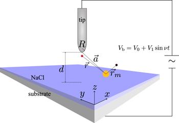
Figure 1. The schematic diagram of the AC STML system. In the dipole approximation, the yellow (black) sphere represents the molecular nucleus (molecular electron). The molecule is separated from the metallic substrate by the decoupling layer. The red sphere stands for the tunneling electron. The radius of the tip apex is R. d represents the distance between the bottom of the tip and the decoupling layer. $\vec{r}$ (${\vec{r}}_{m}$, $\vec{a}$) means the distance from the tunneling electron (molecular electron, the center of the tip's apex) to the nucleus. The AC bias ${V}_{b}\left(t\right)={V}_{0}+{V}_{1}\sin \left(\nu t\right)$ is applied between the tip and the substrate. |
The Hamiltonian in our AC-STML system is divided into three parts,
$\begin{eqnarray}{\hat{H}}_{\mathrm{total}}=\hat{{H}_{\mathrm{el}}}+{\hat{H}}_{m}+{\hat{H}}_{\mathrm{el}-{\rm{m}}},\end{eqnarray}$
where ${\hat{H}}_{\mathrm{el}}=-{{\hslash }}^{2}{{\rm{\nabla }}}^{2}/2{m}_{e}+V\left(\vec{r}\right)$ corresponds to the Hamiltonian of the tunneling electron. me is the electron mass, and $V\left(\vec{r}\right)$ is the potential for the tunneling electron at the position $\vec{r}$. ${\hat{H}}_{m}={E}_{g}\left|{\chi }_{g}\right\rangle \left\langle {\chi }_{g}\right|+{E}_{e}\left|{\chi }_{e}\right\rangle \left\langle {\chi }_{e}\right|$ is the Hamiltonian of the molecule which is simplified as a two-level system [28–30]. $\left|{\chi }_{g}\right\rangle $ is the molecular ground state with energy Eg, and $\left|{\chi }_{e}\right\rangle $ is the molecular excited state with energy Ee. ${\hat{H}}_{\mathrm{el}-{\rm{m}}}\,\simeq -e\hat{\vec{\mu }}\cdot \vec{r}/{\left|\vec{r}\right|}^{3}$ is the Coulomb interaction between the tunneling electron and the molecule. e is the electron charge, and $\hat{\vec{\mu }}$ is the electric dipole moment operator of the molecule [24]. This interaction will induce the molecular transition between its two states in the inelastic tunneling process.The electron wavefunctions in the state k of the tip and in the state n of the substrate are written [31] as
$\begin{eqnarray}\left\langle \vec{r}| {\phi }_{k}\right\rangle ={A}_{k}\displaystyle \frac{{{\rm{e}}}^{-{\kappa }_{k}\left(\left|\vec{r}-\vec{a}\right|-R\right)}}{{\kappa }_{k}\left|\vec{r}-\vec{a}\right|},\end{eqnarray}$
$\begin{eqnarray}\left\langle \vec{r}| {\varphi }_{n}\right\rangle ={B}_{n}{{\rm{e}}}^{-{\kappa }_{n}\left|z\right|},\end{eqnarray}$
where ${\kappa }_{k}=\sqrt{-2{m}_{e}{\xi }_{k}}/{\hslash }$ (${\kappa }_{n}=\sqrt{-2{m}_{e}{E}_{n}}/{\hslash }$) characterizes the decay factor of the tunneling electron with energy ξk (En) in the tip (substrate). Ak and Bn are the normalized coefficients derived from the first-principle calculation [32, 33].At a given bias, both the elastic and the inelastic tunneling occur. The interaction between the molecule and the tunneling electron is small and is treated as a perturbation. Thus the probability of the molecule in its excited state is quite low [34]. At the beginning, we assume that the molecule is in its ground state and the tunneling electron is in the state n of the substrate, i.e., $\left|{\rm{\Psi }}\left(0\right)\right\rangle =\left|{\chi }_{g}\right\rangle \left|{\varphi }_{n}\right\rangle $ noticing the typical low temperature in the STML experiments [7, 8, 18]. Using the time-dependent perturbation theory, we find that at time t, the system evolves to state
$\begin{eqnarray}\begin{array}{rcl}\left|{\rm{\Psi }}\left(t\right)\right\rangle & = & {{\rm{e}}}^{-{\rm{i}}\left({E}_{n}+{E}_{g}\right)t/{\hslash }}\left|{\chi }_{g}\right\rangle \left|{\varphi }_{n}\right\rangle \\ & & +\sum _{k}{c}_{g,k}\left(t\right)\left|{\chi }_{g}\right\rangle \left|{\phi }_{k}\right\rangle +\sum _{k}{c}_{e,k}\left(t\right)\left|{\chi }_{e}\right\rangle \left|{\phi }_{k}\right\rangle ,\end{array}\end{eqnarray}$
where ${c}_{g,k}\left(t\right)$ is the elastic tunneling amplitude and ${c}_{e,k}\left(t\right)$ is the inelastic tunneling amplitude. The dynamical equations of the tunneling amplitudes read $\begin{eqnarray}{\rm{i}}{\hslash }\displaystyle \frac{{\rm{d}}{c}_{g,k}\left(t\right)}{{\rm{d}}t}=\left({\tilde{\xi }}_{k}\left(t\right)+{E}_{g}\right){c}_{g,k}\left(t\right)+{{\rm{e}}}^{-{\rm{i}}\left({\tilde{E}}_{n}+{E}_{g}\right)\displaystyle \frac{t}{{\hslash }}}{{ \mathcal M }}_{n,k},\end{eqnarray}$
$\begin{eqnarray}\begin{array}{rcl}{\rm{i}}{\hslash }\displaystyle \frac{{\rm{d}}{c}_{e,k}\left(t\right)}{{\rm{d}}t} & = & \left({\tilde{\xi }}_{k}\left(t\right)+{E}_{e}\right){c}_{e,k}\left(t\right)\\ & & +{{ \mathcal N }}_{s,t}{| }_{{V}_{b},{E}_{n}\to {\xi }_{k}}{{\rm{e}}}^{-{\rm{i}}\left({\tilde{E}}_{n}+{E}_{g}\right)\displaystyle \frac{t}{{\hslash }}},\end{array}\end{eqnarray}$
where ${{ \mathcal M }}_{n,k}$ is the transition matrix element in the elastic tunneling and ${{ \mathcal N }}_{s,t}{| }_{{V}_{b},{E}_{n}\to {\xi }_{k}}$ is the transition matrix element from the substrate's state to the tip's state under the AC bias Vb [24]. ${\tilde{E}}_{n}$ (${\tilde{\xi }}_{k}$) is the electron energy in the substrate (tip) under the bias. In this work, we apply an AC bias ${V}_{b}\left(t\right)$ between the electrodes. In this case, we have the simple relations, ${\widetilde{\xi }}_{k}={\xi }_{k}+{{eV}}_{0}+{{eV}}_{1}\sin \left(\nu t\right)$ and ${\widetilde{E}}_{n}={E}_{n}$.The inelastic tunneling rate is written as
$\begin{eqnarray}\begin{array}{rcl}\displaystyle \frac{{\rm{d}}}{{\rm{d}}t}{\left|{c}_{e,k}\left(t\right)\right|}^{2} & = & \displaystyle \frac{2}{{{\hslash }}^{2}}{{ \mathcal N }}_{s,t}^{2}{| }_{{V}_{b},{E}_{n}\to {\xi }_{k}}\mathrm{Re}\left\{\Space{0ex}{0.25ex}{0ex}{{\rm{e}}}^{-{\rm{i}}\left[{Bt}-\displaystyle \frac{{{eV}}_{1}}{{\hslash }\nu }\cos \left(\nu t\right)\right]}\right.\\ & & \left.\times {\displaystyle \int }_{0}^{t}{\rm{d}}\tau {{\rm{e}}}^{{\rm{i}}\left[B\tau -\displaystyle \frac{{{eV}}_{1}}{{\hslash }\nu }\cos \left(\nu \tau \right)\right]}\right\},\end{array}\end{eqnarray}$
where we have used the notation $B\equiv \left({\xi }_{k}-{E}_{n}+{E}_{\mathrm{eg}}+{{eV}}_{0}\right)/{\hslash }$. The inelastic electron current is $\begin{eqnarray}{I}_{s,t}\left(t\right)=e\sum _{n,k}{F}_{{\mu }_{0},T}\left({E}_{n}\right)\left[1-{F}_{{\mu }_{0},T}\left({\xi }_{k}\right)\right]\displaystyle \frac{{\rm{d}}}{{\rm{d}}t}{\left|{c}_{e,k}\left(t\right)\right|}^{2},\end{eqnarray}$
where ${F}_{{\mu }_{0},T}\left(E\right)=1/\left\{\exp \left[\left(E-{\mu }_{0}\right)/{k}_{{\rm{B}}}T\right]+1\right\}$ is the Fermi–Dirac distribution of the electron in the tip or substrate at energy E and temperature T. kB is the Boltzmann constant and μ0 is the Fermi energy. The subscript of Is,t means that the tunneling electron passes from the substrate to the tip. In experiments, STML is performed under a very low temperature, e.g., 5 K or 13 K [7, 8, 18]. Therefore, the Fermi–Dirac distribution is simplified as ${F}_{{\mu }_{0},T}\left(E\right)=1$ for E < μ0 and ${F}_{{\mu }_{0},T}\left(E\right)=0$ for E ≥ μ0. The inelastic current is thus rewritten as ${I}_{s,t}\left(t\right)=e{\sum }_{n,k}\tfrac{{\rm{d}}}{{\rm{d}}t}{\left|{c}_{e,k}\left(t\right)\right|}^{2}$.By replacing the summation with the integral and using the Jacobi-Anger expansion ${{\rm{e}}}^{{\rm{i}}a\cos \left(\nu t\right)}={\sum }_{l=-\infty }^{\infty }{{\rm{e}}}^{{\rm{i}}l\pi /2}{J}_{l}\left(a\right){{\rm{e}}}^{{\rm{i}}l\nu t}$, we obtain the inelastic tunneling current explicitly asappendix .
$\begin{eqnarray}\begin{array}{rcl}{I}_{s,t}\left(t\right) & = & {\displaystyle \int }_{-\infty }^{{\mu }_{0}}{\rm{d}}{E}_{n}{\displaystyle \int }_{{\mu }_{0}}^{0}{\rm{d}}{\xi }_{k}{\rho }_{s}\left({E}_{n}\right){\rho }_{t}\left({\xi }_{k}\right)\displaystyle \frac{{\rm{d}}}{{\rm{d}}t}{\left|{c}_{e,k}\left(t\right)\right|}^{2}\\ & = & \displaystyle \frac{2}{{{\hslash }}^{2}}{\displaystyle \int }_{2{\mu }_{0}}^{{\mu }_{0}}{\rm{d}}{E}_{n}{\displaystyle \int }_{{\mu }_{0}}^{0}{\rm{d}}{\xi }_{k}{\rho }_{s}\left({E}_{n}\right){\rho }_{t}\left({\xi }_{k}\right)\\ & & \times {{ \mathcal N }}_{s,t}^{2}{| }_{{V}_{b},{E}_{n}\to {\xi }_{k}}\displaystyle \sum _{l,l^{\prime} =-\infty }^{\infty }{\left(-1\right)}^{l^{\prime} }\\ & & \times {J}_{l}\left(\displaystyle \frac{{{eV}}_{1}}{{\hslash }\nu }\right){J}_{l^{\prime} }\left(\displaystyle \frac{{{eV}}_{1}}{{\hslash }\nu }\right){\left(B-l^{\prime} \nu \right)}^{-1}\\ & & \times \{\cos \left[\left(l-l^{\prime} \right)\nu t+\left(l+l^{\prime} -1\right)\pi /2\right]\\ & & -\cos \left[-\left(B-l\nu \right)t+\left(l+l^{\prime} -1\right)\pi /2\right]\},\end{array}\end{eqnarray}$
where ${\rho }_{s}\left(E\right)$ (ρt$\left(E\right)$) is the density of state in the substrate (tip) at energy E. Eeg = Ee − Eg is the molecular energy gap, and ${J}_{i}\left(x\right)$ is the i-th Bessel function of the first kind. In the derivation above, we have used the property of the Bessel functions ${J}_{i}\left(-a\right)={\left(-1\right)}^{i}{J}_{i}\left(a\right)$. We change the range of the integral about En from $\left[-\infty ,{\mu }_{0}\right]$ to $\left[2{\mu }_{0},{\mu }_{0}\right]$, since most electrons of the metal occupy states near the Fermi energy. The detailed derivations are presented in the 2.2. AC-current in the frequency domain
In a manner different from the DC voltage case, the system under AC bias will not reach a steady state with a constant current at the long-time limit. Instead, the current oscillates with various Fourier frequencies. The information of the energy level can be extracted from these components in the Fourier transformations of ${I}_{s,t}\left(t\right)$ as follows:
$\begin{eqnarray}\begin{array}{rcl}{I}_{s,t}\left(\omega \right) & = & {\displaystyle \int }_{-\infty }^{+\infty }{\rm{d}}t{{\rm{e}}}^{{\rm{i}}\omega t}{I}_{s,t}\left(t\right)\\ & = & \displaystyle \frac{2\pi }{{{\hslash }}^{2}}{\displaystyle \int }_{2{\mu }_{0}}^{{\mu }_{0}}{\rm{d}}{E}_{n}{\displaystyle \int }_{{\mu }_{0}}^{0}{\rm{d}}{\xi }_{k}{\rho }_{s}\left({E}_{n}\right){\rho }_{t}\left({\xi }_{k}\right)\\ & & \times {{ \mathcal N }}_{s,t}^{2}{| }_{{V}_{b},{E}_{n}\to {\xi }_{k}}\displaystyle \sum _{l,l^{\prime} =-\infty }^{\infty }{\left(-1\right)}^{l^{\prime} }\\ & & \times {J}_{l}\left(\displaystyle \frac{{{eV}}_{1}}{{\hslash }\nu }\right){J}_{l^{\prime} }\left(\displaystyle \frac{{{eV}}_{1}}{{\hslash }\nu }\right){\left(B-l^{\prime} \nu \right)}^{-1}\\ & & \times \{\delta \left[\left(l-l^{\prime} \right)\nu +\omega \right]{{\rm{e}}}^{{\rm{i}}\left(l+l^{\prime} -1\right)\pi /2}\\ & & +\delta \left[\left(l-l^{\prime} \right)\nu -\omega \right]{{\rm{e}}}^{-{\rm{i}}\left(l+l^{\prime} -1\right)\pi /2}\\ & & -\delta \left[\left(B-l\nu \right)+\omega \right]{{\rm{e}}}^{-{\rm{i}}\left(l+l^{\prime} -1\right)\pi /2}\\ & & -\delta \left[\left(B-l\nu \right)-\omega \right]{{\rm{e}}}^{{\rm{i}}\left(l+l^{\prime} -1\right)\pi /2}\}.\end{array}\end{eqnarray}$
Here, we have used the relation ${\int }_{-\infty }^{+\infty }{\rm{d}}t{{\rm{e}}}^{{\rm{i}}{\rm{\Omega }}t}=2\pi \delta \left({\rm{\Omega }}\right)$.The photon count in the AC system heavily depends on the AC inelastic tunneling current that we calculated above. As the molecule is firstly excited to its excited state by the AC bias and then decays back through the spontaneous emission process, the population equation of the molecule excited state reads [24] ${\dot{P}}_{e}\left(t\right)=-\gamma {P}_{e}\left(t\right)+{I}_{s,t}\left(t\right)$, where ${P}_{e}\left(t\right)$ stands for the excited-state population and γ is the spontaneous decay rate. Since the AC inelastic tunneling current oscillates with various Fourier frequencies, we divide the excited-state population ${P}_{e}\left(t\right)$ with respect to the Fourier frequencies, i.e., $-{\rm{i}}\omega {P}_{e}\left(\omega \right)=-\gamma {P}_{e}\left(\omega \right)+{I}_{s,t}\left(\omega \right)$ where ${P}_{e}\left(\omega \right)={\int }_{-\infty }^{\infty }{P}_{e}\left(t\right){{\rm{e}}}^{{\rm{i}}\omega t}{\rm{d}}t$. Thus, the zero-component current contributes to a steady photon count in the long-time limit while every non-zero-frequency component gives one time-dependent photon count with its corresponding frequency.
To find the energy levels, we consider the zero-frequency component of the inelastic current (equation (10 )), i.e., ω = 0 as11 ) retains the current for the case with a DC voltage (V1 = 0) obtained in [24] by noticing that J0(0) = 1 and Jl(0) = 0 for any l ≠ 0. In the paper [24], the current caused by the DC bias is kept constant at the long-time limit, while in our AC case, the inelastic current oscillates with time and cannot reach a steady state. So we make a Fourier transformation of the AC-induced current and investigate the zero-frequency component of the current. In the long-time limit, the time-independent photon count is proportional to the zero-component current, i.e., equation (11 ).
$\begin{eqnarray}\begin{array}{rcl}{I}_{s,t}\left(\omega =0\right) & = & \displaystyle \frac{4\pi }{{{\hslash }}^{2}}{\displaystyle \int }_{2{E}_{f}}^{{E}_{f}}{\rm{d}}{E}_{n}{\displaystyle \int }_{{E}_{f}}^{0}{\rm{d}}{\xi }_{k}{\rho }_{s}\left({E}_{n}\right){\rho }_{t}\left({\xi }_{k}\right)\\ & & \times {{ \mathcal N }}_{s,t}^{2}{| }_{{V}_{b},{E}_{n}\to {\xi }_{k}}\displaystyle \sum _{l,l^{\prime} =-\infty }^{\infty }{\left(-1\right)}^{l^{\prime} }\\ & & \times {J}_{l}\left(\displaystyle \frac{{{eV}}_{1}}{{\hslash }\nu }\right){J}_{l^{\prime} }\left(\displaystyle \frac{{{eV}}_{1}}{{\hslash }\nu }\right){\left(B-l^{\prime} \nu \right)}^{-1}\\ & & \times \cos \left[\left(l+l^{\prime} -1\right)\pi /2\right]\\ & & \times \left\{\delta \left[\left(l-l^{\prime} \right)\nu \right]-\delta \left(B-l\nu \right)\right\}.\end{array}\end{eqnarray}$
The result shown in equation (3. Results
To reveal the resonant conditions in the above current, we perform the numerical calculation of the tunneling current with parameters extracted from the experimental setup. In the STML experiments, the metal used for the tip and the substrate is typically chosen as gold (Au) [35–39], silver (Ag) [1, 29, 30, 40–46] and copper (Cu) [11, 18, 47, 48]. In our simulation of the STML current, the tip and the substrate are made of silver with Fermi energy μ0 = − 4.64 eV. The calculation of the current requires the Ag's density of state, which is obtained from the book [49] by the spline interpolation of the discrete data points. The detail of the obtained density of state was presented in our previous publications [24, 50]. In the experiments, the molecular gap is typically chosen to be around 1.5 eV ∼ 4 eV [1, 29, 38, 42, 43, 51–53] to avoid the possible damage caused by the strong static electric field between the tip and the substrate. For example, the energy gap between the first single excited state and the ground state of the free-base phthalocyanine (H2Pc) molecule is 1.81 eV[42, 51], and the $Q\left(0,0\right)$ transition energy of the zinc-phthalocyanine (ZnPc) molecule is 1.90 eV [1, 29, 38, 43, 52, 53]. Here, we choose that the molecular gap is Eeg = 2.0 eV. In the scanning process, the distance d between the tip and the substrate is typically around several nanometers. And we have used d = 0.5 nm and the radius of the tip apex is R = 0.5 nm.
3.1. Tunneling current for the tip position $\overrightarrow{a}=\left(0,0,d\right)$
Since the absolute value of the Bessel function decreases as its order increases, it is reasonable to cut off the high order term of the Bessel function of the summation in equation (11 ). Noticing that the factor $\cos \left[\left(l+l^{\prime} -1\right)\pi /2\right]$ vanishes for the case where $l+l^{\prime} $ is even, we consider the cutoffs with $\left|l-l^{\prime} \right|\leqslant 3$ and $\left|l-l^{\prime} \right|\leqslant 5$ to check the convergence of the current in equation (11 ). Figure 2(a) shows the zero-frequency inelastic tunneling current as a function of AC frequency ν. The parameters in the simulation are given as follows, $l\,\in \left[-3,3\right],R=0.5\,\mathrm{nm},\,d=0.5\,\mathrm{nm}$, $\vec{a}=\left(0,0,d\right)$, Eeg = 2 eV, eV1/ℏν = 2, μ0 = − 4.64 eV and eV0 = − 1.88 eV. The tip is placed right above the molecule. In figure 2(a), the red dotted line reveals the current including the summation of $\left|l\right|\leqslant 3$ and $\left|l-l^{\prime} \right|\leqslant 3$, and the black line shows that of $\left|l\right|\leqslant 3$ and $\left|l-l^{\prime} \right|\leqslant 5$. The coincidence of the two curves demonstrates that the zero-frequency inelastic current already converges with $\left|l-l^{\prime} \right|=3$ and $\left|l\right|\leqslant 3$. Therefore, we use the cutoff $\left|l\right|\leqslant 3$ and $\left|l-l^{\prime} \right|\leqslant 3$ in the following calculation.

Figure 2. (a) The convergency of the zero-frequency inelastic current with $\vec{a}=\left(0,0,d\right)$. The red dotted (blue dashed) curve shows the current under the summation of $\left|l\right|\leqslant 3$ and $\left|l-l^{\prime} \right|\leqslant 3$ ($\left|l-l^{\prime} \right|\leqslant 5$). Both lines show the non-analyticity of the current with respect to the oscillating frequency. (b) The first derivative of the zero-frequency inelastic current with respect to the oscillating frequency ν. The tip is placed right above the molecule. The red dots show the discontinuous data in the current, which correspond to ℏν = 0.04, 0.06, and 0.12 eV. We have chosen the parameters as l ∈ [ − 3, 3], R = 0.5 nm, d = 0.5 nm, $\vec{a}=\left(0,0,d\right)$, Eeg = 2 eV, μ0 = − 4.64 eV, and eV0 = − 1.88 eV. The ratio of the time-dependent voltage amplitude over the oscillating frequency is fixed at eV1/ℏν = 2. |
The curve in figure 2(a) also shows the discrete knee points. We numerically calculate the first derivative of the inelastic tunneling current ${I}_{s,t}\left(\omega =0\right)$ with respect to the AC frequency ν and plot the result in figure 2(b). In figure 2(b), the line reveals the discontinuity of the first derivative of the zero-frequency current with the discontinuous spots located at ℏν = 0.04 eV, 0.06 eV, and 0.12 eV. By defining the detuning Δ = Eeg + eV0, we find that the discontinuous spots are in agreement with the condition ${\rm{\Delta }}-l^{\prime} {\hslash }\nu =0$ with $l^{\prime} \,=3,2,1$, respectively. Mathematically, such discontinuous behavior can be understood with the Jacobi-Anger expansion. The STML system with AC bias ${V}_{0}+{V}_{1}\sin \left(\nu t\right)$ is equivalent to the system with a series of DC biases ${V}_{l}^{\mathrm{eff}}={V}_{0}-l^{\prime} {\hslash }\nu /e$ ($l^{\prime} =0,\pm 1,\pm 2,\ldots $). Once one effective bias ${V}_{l}^{\mathrm{eff}}$ matches the molecular energy gap, namely ${V}_{l}^{\mathrm{eff}}={E}_{\mathrm{eg}}$, a new contribution to the molecular excitation rate (the inelastic current) emerges and results in one discontinuous point in its first derivative curve. Therefore we have demonstrated that the discontinuous spots reveal the fine detail of the molecule.
To investigate the influence caused by the height of the tip, we choose the parameters d = 0.3 nm, d = 0.4 nm and d = 0.5 nm respectively. Figure 3(a) shows the zero-frequency component of the inelastic current which is dependent upon the position of the tip. The green, yellow and red curves correspond to the inelastic current with the tip fixed at d = 0.3 nm, d = 0.4 nm and d = 0.5 nm respectively. The inelastic current becomes larger as the tip moves to the molecule. Because we modeled the electron wavefunction of the tip as equation (2 ), which decays with the tip radius exponentially, when the STM tip approaches the substrate, the electron wavefunction at the position of the tunneling electron increases, resulting in the increase of the transition matrix element. Finally, the inelastic current increases. Figure 3(b) reveals the first derivative of the inelastic current with respect to the frequency. Discontinuous data are marked by a dot. All the curves have discontinuous data at the same spots ℏν = 0.04 eV, 0.06 eV, and 0.12 eV, which are in agreement with the condition ${\rm{\Delta }}-l^{\prime} {\hslash }\nu =0$. Although the inelastic current changes with the tip approaching the molecule, the knee points of the current satisfy the resonant condition which is independent of the position of the tip.
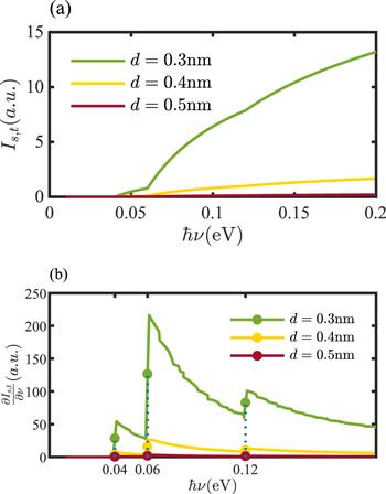
Figure 3. (a) The zero-frequency component of the inelastic current with different heights of the tip. The green, yellow and red curves correspond to the inelastic current with d = 0.3 nm, d = 0.4 nm and d = 0.5 nm respectively. (b) The first derivative of the zero-frequency inelastic current with respect to the frequency ν. The tip is placed right above the molecule. The dotted markers in (b) show the discontinuous data at ℏν = 0.04 eV, 0.06 eV, and 0.12 eV. The other parameters are the same as before. |
The advantage of our AC-STML is that the frequency can be tuned with precision. In the DC bias case, the inelastic tunneling current has a sudden rise from zero when the absolute value of the DC bias becomes equal to a critical quantity, i.e., the absolute value of the molecular energy gap divided by the electron charge [24]. And one can extract the information of the molecular energy gap from this curve theoretically. However, due to the noise of the experiment, the inelastic tunneling current curve changes smoothly near the critical quantity. Thus one can only read out the energy gap roughly. In the AC STML method, the point of the energy gap is featured as the knee point of the zero-frequency component of the AC current. These points show a discontinuous and non-analytical property at the non-zero point of the current curve. By numerically calculating the first derivative of the zero-frequency component of the inelastic tunneling current with respect to the AC frequency, the discontinuous points, i.e., the sudden rising points, correspond to the points of energy resonance. We can read out discontinuous points directly and then obtain the energy gap of the molecule.
The method of realizing our proposal has two steps. Firstly, the molecule is probed via a DC bias. The molecular energy gap can be roughly obtained through the rising point in the photon-emission spectrum. And we estimate the rough value as V0. Second, we add a non-zero AC component to this DC voltage and apply this time-dependent bias to the molecule. A series of knee points can be shown in the figure of the zero-frequency inelastic tunneling current ${I}_{s,t}\left(\omega =0\right)$ as a function of the AC frequency. Then, we can precisely determine these non-analytical points through the first derivative of the inelastic tunneling current ${I}_{s,t}\left(\omega =0\right)$ with respect to the AC frequency. The precise molecular gap is given with the relation ${E}_{\mathrm{eg}}-e\left|{V}_{0}\right|=l^{\prime} {\hslash }\nu \left(l^{\prime} =0,\pm 1,\pm 2,\pm 3\right)$.
3.2. Tunneling current for the tip position $\overrightarrow{a}\,=\left(0.2\,\mathrm{nm},0,d\right)$
Without loss of generality, we consider the case where the tip is laterally displaced from the center of the molecule, e.g., $\vec{a}=\left(0.2\,\mathrm{nm},0,d\right)$. We calculate the zero-frequency inelastic current as shown in figure 4(a). The curve shows the same feature as that in figure 2(a). The other parameters in figure 4 are the same as in figure 2. The coincidence between the red dotted line and the blue dashed line also shows the convergence of our calculation when we consider the summation with terms $\left|l\right|\leqslant 3$ and $\left|l-l^{\prime} \right|\leqslant 3$. We also calculate the first derivative of the zero-frequency inelastic current with respect to the AC frequency to explore the fine details of the current. As shown in figure 4(b) , the first derivative of the zero-frequency inelastic current reveals the discontinuity at the same spots ℏν = 0.04 eV, 0.06 eV, and 0.12 eV. The results in $\vec{a}=\left(0,0,d\right)$ and $\vec{a}=\left(0.2\,\mathrm{nm},0,d\right)$ indicates that the fine structure in the AC current is robust with respect to the relative position between the tip and the molecule.
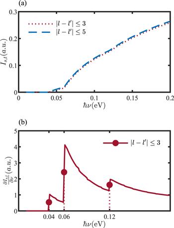
Figure 4. (a) The convergence of the zero-frequency inelastic current in $\vec{a}=\left(0.2\,\mathrm{nm},0,d\right)$. The red dotted line and the blue dashed line correspond to the condition $\left|l-l^{\prime} \right|\leqslant 3$ and $\left|l-l^{\prime} \right|\leqslant 5$, respectively. (b) The first-order derivative of the zero-frequency inelastic current about the bias frequency ν in $\vec{a}=\left(0.2\,\mathrm{nm},0,d\right)$. The other parameters are the same as before. |
To investigate the influence of the relative position of the tip and the molecule on the inelastic current, we calculated the zero-frequency component of the current and its first derivative with respect to the frequency as a function of the frequency in figure 5. Since we assume that the molecular dipole is isotropic in three axes, the inelastic current is symmetric around the z-axis. Hence, we only calculate the displacement of the tip in the x-axis. In figure 5, the red, blue and yellow curves correspond to the cases with $\vec{a}=\left(0,0,d\right)$, $\vec{a}=\left(0.1\,\mathrm{nm},0,d\right)$ and $\vec{a}=\left(0.2\,\mathrm{nm},0,d\right)$ respectively. In figure 5(a), when the tip is right above the molecule, the zero-frequency inelastic current is much smaller than in the other cases. The current with $\vec{a}=\left(0.1\,\mathrm{nm},0,d\right)$ is a little smaller than the current with $\vec{a}=\left(0.2\,\mathrm{nm},0,d\right)$. So, the inelastic current can change with the distance between the tip and the molecule. In figure 5(b), the dotted markers reveal the knee points of the current at the same spots ℏν = 0.04 eV, 0.06 eV, and 0.12 eV, showing that the resonant relation is independent on the relative of the tip and the molecule.
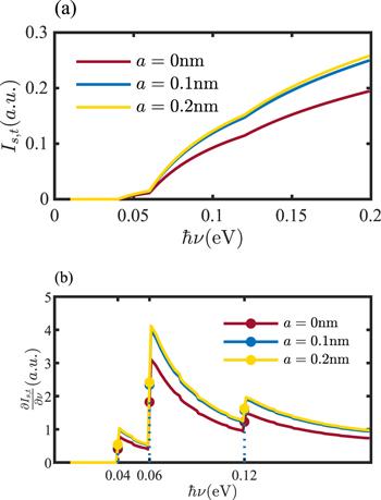
Figure 5. (a) The zero-frequency component of the inelastic tunneling current as a function of the frequency with the lateral displacement between the tip and the molecule fixed at $\vec{a}=\left(0,0,d\right)$, $\vec{a}=\left(0.1\,\mathrm{nm},0,d\right)$ and $\vec{a}=\left(0.2\,\mathrm{nm},0,d\right)$, which is represented by the red, blue and yellow curves respectively. (b) The first derivative of the zero-frequency component of the current with respect to the frequency. The correspondence between the color and the lateral displacement is the same as (a). The dotted markers show the discontinuous spots in curves. The other parameters are the same as before. |
To show the general case, we calculate the inelastic tunneling current and its first derivative with different energy detuning Δ = 0.04, 0.06, 0.08, 0.1, and 0.12 eV, as illustrated in figure 6. The left column represents the current curves with an upward trend as discussed before. When the frequency ν of the bias is small, the energy of the tunneling electron is too weak to excite the molecule. No inelastic tunneling electron transfers energy to the molecule and no inelastic current flows through the electrodes. The energy of the rising point in the current becomes higher as Δ increases. From the definition Δ = Eeg + eV0, the increase of V0 causes the effective bias $l^{\prime} {\hslash }\nu /e-{V}_{0}$ to decrease. To reach the molecular excitation energy, the value of ℏν should be larger. The right column in figure 6 plots the first derivative of the current. The round (square, triangle) spot reveals the non-analysis feature of the current. With Δ increasing, the energy of the knee point in the same shape increases too.
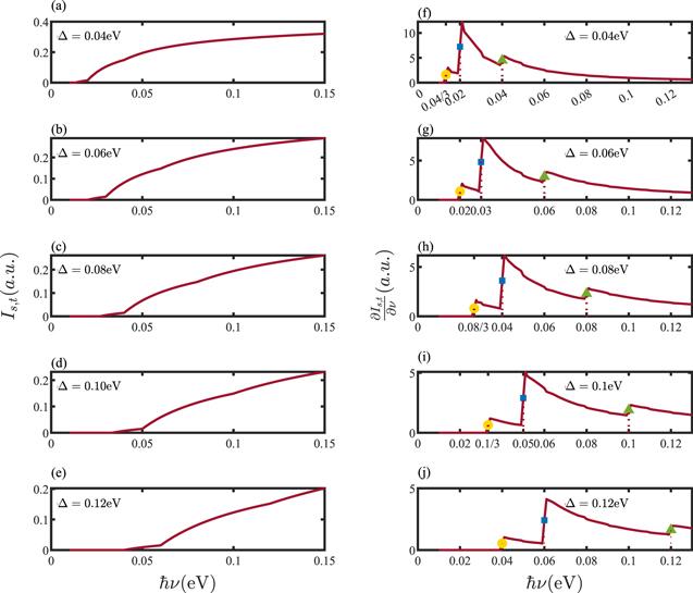
Figure 6. The inelastic tunneling current and its first derivative in $\vec{a}=\left(0.2\,\mathrm{nm},0,d\right)$ with Δ = 0.04, 0.06, 0.08, 0.1, and 0.12 eV. (a)–(e) show the inelastic tunneling current with an upward trend. (f)–(j) give the first derivative of the current. The round (square, triangle) dot characterizes the discontinuous points. |
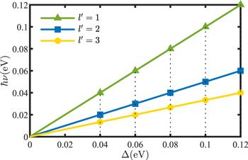
To figure out the relation between the energy of knee points and Δ, we show the energy of knee points as the function of the energy Δ with various orders. Figure 7 plots the energy of spots with the same markers in figure 6. The energy of the knee points linearly increases with energy Δ. The slope of the line with triangle (square, round) markers is 1 (1/2, 1/3), and matches $1/l^{\prime} $ in the relation ${\rm{\Delta }}-l^{\prime} {\hslash }\nu =0$ with $l^{\prime} =1\left(2,3\right)$. This demonstrates that the molecular gap Eeg can be determined via the knee points ${\rm{\Delta }}-l^{\prime} {\hslash }\nu =0$.
Figure 7. The energy of knee points as a function of Δ = Eeg + eV0. The data points in round (square, triangle) dots correspond to the knee points with the same marker in figure 6. The slope of the triangle (square, round) dot line equals to $1/l^{\prime} =1\left(1/2,1/3\right)$. |
4. Conclusions
In summary, we have proposed the AC-STML setup to measure fine molecular structures. We calculate the photon count reflected by the inelastic current and obtain its Fourier components at the long-time limit. We show that the rising position of the current spectrum is precisely determined by the match between the effective bias and the molecular energy gap. These rising positions are utilized to find the molecular energy levels by scanning the frequency of the AC bias. The observations here allow us to propose an alternative method to determine the molecular levels, especially the fine structures around electronic levels, e.g., the vibrational levels.
The AC-STML method can be realized in experiments. Theoretically, our proposal works well in a large range of AC frequencies. In reality, the AC frequency can be realized around the GHz level [54]. Therefore, as long as we can localize the rough bias V0 to the range $\left|{E}_{\mathrm{eg}}-e\left|{V}_{0}\right|\right|\leqslant 10\mu $ eV through the inelastic current curve in the DC bias case, the precise energy gap will be obtained successfully.
Appendix. The derivation of the AC current
The first derivative of the inelastic tunneling amplitude ${c}_{e,k}\left(t\right)$
$\begin{eqnarray*}\begin{array}{rcl}{\rm{i}}{\hslash }\displaystyle \frac{{\rm{d}}{c}_{e,k}\left(t\right)}{{\rm{d}}t} & = & \left({\tilde{\xi }}_{k}\left(t\right)+{E}_{e}\right){c}_{e,k}\left(t\right)\\ & & +{{ \mathcal N }}_{s,t}{| }_{{V}_{b},{E}_{n}\to {\xi }_{k}}{{\rm{e}}}^{-{\rm{i}}\left({\tilde{E}}_{n}+{E}_{g}\right)\displaystyle \frac{t}{{\hslash }}}.\end{array}\end{eqnarray*}$
By using the relation ${\widetilde{\xi }}_{k}={\xi }_{k}+{{eV}}_{0}+{{eV}}_{1}\sin \left(\nu t\right)$ and ${\widetilde{E}}_{n}={E}_{n}$, we rewrite the inelastic tunneling amplitude ${c}_{e,k}\left(t\right)$ as $\begin{eqnarray*}\begin{array}{rcl}\displaystyle \frac{{\rm{d}}{c}_{e,k}\left(t\right)}{{\rm{d}}t} & = & \displaystyle \frac{1}{{\rm{i}}{\hslash }}\left[{\xi }_{k}+{{eV}}_{0}+{{eV}}_{1}\sin \left(\nu t\right)+{E}_{e}\right]{c}_{e,k}\left(t\right)\\ & & +\displaystyle \frac{1}{{\rm{i}}{\hslash }}{{ \mathcal N }}_{s,t}{| }_{{V}_{b},{E}_{n}\to {\xi }_{k}}{{\rm{e}}}^{-{\rm{i}}\left({E}_{n}+{E}_{g}\right)\displaystyle \frac{t}{{\hslash }}}.\end{array}\end{eqnarray*}$
The solution of the inelastic tunneling amplitude ${c}_{e,k}\left(t\right)$ is $\begin{eqnarray*}\begin{array}{rcl}{c}_{e,k}\left(t\right) & = & \displaystyle \frac{1}{{\rm{i}}{\hslash }}{{ \mathcal N }}_{s,t}{| }_{{V}_{b},{E}_{n}\to {\xi }_{k}}{{\rm{e}}}^{-{\rm{i}}\left[\left({\xi }_{k}+{E}_{e}+{{eV}}_{0}\right)\displaystyle \frac{t}{{\hslash }}-\displaystyle \frac{{{eV}}_{1}}{{\hslash }\nu }\cos \left(\nu t\right)\right]}\\ & & \times {\displaystyle \int }_{0}^{t}{\rm{d}}\tau {{\rm{e}}}^{{\rm{i}}\left[\left({\xi }_{k}-{E}_{n}+{E}_{\mathrm{eg}}+{{eV}}_{0}\right)\displaystyle \frac{\tau }{{\hslash }}-\displaystyle \frac{{{eV}}_{1}}{{\hslash }\nu }\cos \left(\nu \tau \right)\right]}.\end{array}\end{eqnarray*}$
The inelastic tunneling rate can be expressed as $\begin{eqnarray*}\begin{array}{rcl}\displaystyle \frac{{\rm{d}}{\left|{c}_{e,k}\left(t\right)\right|}^{2}}{{\rm{d}}t} & = & \displaystyle \frac{{\rm{d}}}{{\rm{d}}t}\left[{c}_{e,k}\left(t\right)\cdot {c}_{e,k}^{* }\left(t\right)\right]\\ & = & \displaystyle \frac{{\rm{d}}{c}_{e,k}^{* }\left(t\right)}{{\rm{d}}t}\cdot {c}_{e,k}\left(t\right)+c.c\\ & = & \left\{-\displaystyle \frac{1}{{\rm{i}}{\hslash }}\left[{\xi }_{k}+{{eV}}_{0}+{{eV}}_{1}\sin \left(\nu t\right)+{E}_{e}\right]{c}_{e,k}^{* }\left(t\right)\right.\\ & & \left.-\displaystyle \frac{1}{{\rm{i}}{\hslash }}{{ \mathcal N }}_{s,t}^{* }{| }_{{V}_{b},{E}_{n}\to {\xi }_{k}}{{\rm{e}}}^{{\rm{i}}\left({E}_{n}+{E}_{g}\right)\displaystyle \frac{t}{{\hslash }}}\right\}\cdot {c}_{e,k}\left(t\right)+c.c\\ & = & -\displaystyle \frac{1}{{\rm{i}}{\hslash }}{{ \mathcal N }}_{s,t}^{* }{| }_{{V}_{b},{E}_{n}\to {\xi }_{k}}{{\rm{e}}}^{{\rm{i}}\left({E}_{n}+{E}_{g}\right)\displaystyle \frac{t}{{\hslash }}}{c}_{e,k}\left(t\right)+c.c.\end{array}\end{eqnarray*}$
By substituting the inelastic tunneling amplitude ${c}_{e,k}\left(t\right)$ into the inelastic tunneling rate ${\rm{d}}{\left|{c}_{e,k}\left(t\right)\right|}^{2}/{\rm{d}}t$, we have $\begin{eqnarray}\begin{array}{rcl}\displaystyle \frac{{\rm{d}}{\left|{c}_{e,k}\left(t\right)\right|}^{2}}{{\rm{d}}t} & = & \displaystyle \frac{1}{{{\hslash }}^{2}}{{ \mathcal N }}_{s,t}^{2}{| }_{{V}_{b},{E}_{n}\to {\xi }_{k}}{{\rm{e}}}^{{\rm{i}}\left({E}_{n}+{E}_{g}\right)\displaystyle \frac{t}{{\hslash }}}\\ & & \times {{\rm{e}}}^{-{\rm{i}}\left[\left({\xi }_{k}+{E}_{e}+{{eV}}_{0}\right)\displaystyle \frac{t}{{\hslash }}-\displaystyle \frac{{{eV}}_{1}}{{\hslash }\nu }\cos \left(\nu t\right)\right]}\\ & & \times {\displaystyle \int }_{0}^{t}{\rm{d}}\tau {{\rm{e}}}^{{\rm{i}}\left[\left({\xi }_{k}-{E}_{n}+{E}_{\mathrm{eg}}+{{eV}}_{0}\right)\displaystyle \frac{\tau }{{\hslash }}-\displaystyle \frac{{{eV}}_{1}}{{\hslash }\nu }\cos \left(\nu \tau \right)\right]}+c.c\\ & = & \displaystyle \frac{1}{{{\hslash }}^{2}}{{ \mathcal N }}_{s,t}^{2}{| }_{{V}_{b},{E}_{n}\to {\xi }_{k}}\\ & & \times {{\rm{e}}}^{-{\rm{i}}\left[\left({\xi }_{k}+{E}_{\mathrm{eg}}+{{eV}}_{0}-{E}_{n}\right)\displaystyle \frac{t}{{\hslash }}-\displaystyle \frac{{{eV}}_{1}}{{\hslash }\nu }\cos \left(\nu t\right)\right]}\\ & & \times {\displaystyle \int }_{0}^{t}{\rm{d}}\tau {{\rm{e}}}^{{\rm{i}}\left[\left({\xi }_{k}-{E}_{n}+{E}_{\mathrm{eg}}+{{eV}}_{0}\right)\displaystyle \frac{\tau }{{\hslash }}-\displaystyle \frac{{{eV}}_{1}}{{\hslash }\nu }\cos \left(\nu \tau \right)\right]}+c.c.\end{array}\end{eqnarray}$
Then equation (12 )can be rewritten as
$\begin{eqnarray*}\begin{array}{rcl}\displaystyle \frac{{\rm{d}}{\left|{c}_{e,k}\left(t\right)\right|}^{2}}{{\rm{d}}t} & = & \displaystyle \frac{1}{{{\hslash }}^{2}}{{ \mathcal N }}_{s,t}^{2}{| }_{{V}_{b},{E}_{n}\to {\xi }_{k}}{{\rm{e}}}^{-{\rm{i}}\left[{Bt}-\displaystyle \frac{{{eV}}_{1}}{{\hslash }\nu }\cos \left(\nu t\right)\right]}\\ & & \times {\displaystyle \int }_{0}^{t}{\rm{d}}\tau {{\rm{e}}}^{{\rm{i}}\left[B\tau -\displaystyle \frac{{{eV}}_{1}}{{\hslash }\nu }\cos \left(\nu \tau \right)\right]}+c.c\\ & = & \displaystyle \frac{2}{{{\hslash }}^{2}}{{ \mathcal N }}_{s,t}^{2}{| }_{{V}_{b},{E}_{n}\to {\xi }_{k}}\mathrm{Re}\left\{\Space{0ex}{0.25ex}{0ex}{{\rm{e}}}^{-{\rm{i}}\left[{Bt}-\displaystyle \frac{{{eV}}_{1}}{{\hslash }\nu }\cos \left(\nu t\right)\right]}\right.\\ & & \left.\times {\displaystyle \int }_{0}^{t}{\rm{d}}\tau {{\rm{e}}}^{{\rm{i}}\left[B\tau -\displaystyle \frac{{{eV}}_{1}}{{\hslash }\nu }\cos \left(\nu \tau \right)\right]}\right\},\end{array}\end{eqnarray*}$
where we have defined the notation $B\equiv \left({\xi }_{k}-{E}_{n}\,+\,{E}_{\mathrm{eg}}\,+\,{{eV}}_{0}\right)/{\hslash }$.Using the Jacobi-Anger expansion ${{\rm{e}}}^{{\rm{i}}a\cos \left(\nu t\right)}=\displaystyle \sum _{l=-\infty }^{\infty }{{\rm{e}}}^{{\rm{i}}l\pi /2}{J}_{l}\left(a\right){{\rm{e}}}^{{\rm{i}}l\nu t}$ we have
$\begin{eqnarray*}\begin{array}{rcl}{{\rm{e}}}^{{\rm{i}}\displaystyle \frac{{{eV}}_{1}}{{\hslash }\nu }\cos \left(\nu t\right)} & = & \displaystyle \sum _{l=-\infty }^{\infty }{{\rm{e}}}^{{\rm{i}}l\pi /2}{J}_{l}\left(\displaystyle \frac{{{eV}}_{1}}{{\hslash }\nu }\right){{\rm{e}}}^{{\rm{i}}l\nu t},\\ {{\rm{e}}}^{-{\rm{i}}\displaystyle \frac{{{eV}}_{1}}{{\hslash }\nu }\cos \left(\nu t\right)} & = & {{\rm{e}}}^{-{\rm{i}}\displaystyle \frac{{{eV}}_{1}}{{\hslash }\nu }\cos \left(-\nu t\right)}\\ & = & \sum _{l=-\infty }^{\infty }{{\rm{e}}}^{{\rm{i}}l\pi /2}{J}_{l}\left(-\displaystyle \frac{{{eV}}_{1}}{{\hslash }\nu }\right){{\rm{e}}}^{-{\rm{i}}l\nu t}.\end{array}\end{eqnarray*}$
The inelastic tunneling rate can be expressed through the series of Bessel's function
$\begin{eqnarray}\begin{array}{rcl}\displaystyle \frac{{\rm{d}}{\left|{c}_{e,k}\left(t\right)\right|}^{2}}{{\rm{d}}t} & = & \displaystyle \frac{2}{{{\hslash }}^{2}}{{ \mathcal N }}_{s,t}^{2}{| }_{{V}_{b},{E}_{n}\to {\xi }_{k}}\\ & & \times \displaystyle \sum _{l,l^{\prime} =-\infty }^{\infty }\mathrm{Re}\left\{{{\rm{e}}}^{-{\rm{i}}{Bt}}{{\rm{e}}}^{{\rm{i}}l\pi /2}{J}_{l}\left(\displaystyle \frac{{{eV}}_{1}}{{\hslash }\nu }\right){{\rm{e}}}^{{\rm{i}}l\nu t}\right.\\ & & \left.\times {\displaystyle \int }_{0}^{t}{\rm{d}}\tau {{\rm{e}}}^{{\rm{i}}B\tau }{{\rm{e}}}^{{\rm{i}}l^{\prime} \pi /2}{J}_{l^{\prime} }\left(-\displaystyle \frac{{{eV}}_{1}}{{\hslash }\nu }\right){{\rm{e}}}^{-{\rm{i}}l^{\prime} \nu \tau }\right\}\\ & = & \displaystyle \frac{2}{{{\hslash }}^{2}}{{ \mathcal N }}_{s,t}^{2}{| }_{{V}_{b},{E}_{n}\to {\xi }_{k}}\\ & & \times \displaystyle \sum _{l,l^{\prime} =-\infty }^{\infty }{\left(-1\right)}^{l^{\prime} }{J}_{l}\left(\displaystyle \frac{{{eV}}_{1}}{{\hslash }\nu }\right){J}_{l^{\prime} }\left(\displaystyle \frac{{{eV}}_{1}}{{\hslash }\nu }\right)\\ & & \times \mathrm{Re}\left\{{{\rm{e}}}^{-{\rm{i}}\left(B-l\nu \right)t}{{\rm{e}}}^{{\rm{i}}\left(l+l^{\prime} \right)\pi /2}{\displaystyle \int }_{0}^{t}{\rm{d}}\tau {{\rm{e}}}^{{\rm{i}}\left(B-l^{\prime} \nu \right)\tau }\right\},\end{array}\end{eqnarray}$
where we have used the relation ${J}_{l}\left(-a\right)={\left(-1\right)}^{l}{J}_{l}\left(a\right)$. Calculating the integral, we obtain $\begin{eqnarray}\begin{array}{rcl}\displaystyle \frac{{\rm{d}}{\left|{c}_{e,k}\left(t\right)\right|}^{2}}{{\rm{d}}t} & = & \displaystyle \frac{2}{{{\hslash }}^{2}}{{ \mathcal N }}_{s,t}^{2}{| }_{{V}_{b},{E}_{n}\to {\xi }_{k}}\displaystyle \sum _{l,l^{\prime} =-\infty }^{\infty }{\left(-1\right)}^{l^{\prime} }\\ & & \times {J}_{l}\left(\displaystyle \frac{{{eV}}_{1}}{{\hslash }\nu }\right){J}_{l^{\prime} }\left(\displaystyle \frac{{{eV}}_{1}}{{\hslash }\nu }\right){\left(B-l^{\prime} \nu \right)}^{-1}\\ & & \times \mathrm{Re}\left\{{{\rm{e}}}^{{\rm{i}}\left[\left(l-l^{\prime} \right)\nu t+\left(l+l^{\prime} -1\right)\pi /2\right]}\right.\\ & & \left.-{{\rm{e}}}^{{\rm{i}}\left[-\left(B-l\nu \right)t+\left(l+l^{\prime} -1\right)\pi /2\right]}\right\}\\ & = & \displaystyle \frac{2}{{{\hslash }}^{2}}{{ \mathcal N }}_{s,t}^{2}{| }_{{V}_{b},{E}_{n}\to {\xi }_{k}}\displaystyle \sum _{l,l^{\prime} =-\infty }^{\infty }{\left(-1\right)}^{l^{\prime} }\\ & & \times {J}_{l}\left(\displaystyle \frac{{{eV}}_{1}}{{\hslash }\nu }\right){J}_{l^{\prime} }\left(\displaystyle \frac{{{eV}}_{1}}{{\hslash }\nu }\right){\left(B-l^{\prime} \nu \right)}^{-1}\\ & & \times \left\{\cos \left[\left(l-l^{\prime} \right)\nu t+\left(l+l^{\prime} -1\right)\pi /2\right]\right.\\ & & \left.-\cos \left[-\left(B-l\nu \right)t+\left(l+l^{\prime} -1\right)\pi /2\right]\right\}.\end{array}\end{eqnarray}$
The inelastic current is ${I}_{s,t}\left(t\right)=e{\sum }_{n,k}\tfrac{{\rm{d}}}{{\rm{d}}t}{\left|{c}_{e,k}\left(t\right)\right|}^{2}$.
By replacing the summation with the integral and substituting the inelastic tunneling rate equation (14 ) into the current above Is,t$\left(t\right)$, we obtain the inelastic tunneling current explicitly (equation (9 ) in the main text) as
$\begin{eqnarray}\begin{array}{rcl}{I}_{s,t}\left(t\right) & = & {\displaystyle \int }_{-\infty }^{{\mu }_{0}}{\rm{d}}{E}_{n}{\displaystyle \int }_{{\mu }_{0}}^{0}{\rm{d}}{\xi }_{k}{\rho }_{s}\left({E}_{n}\right){\rho }_{t}\left({\xi }_{k}\right)\displaystyle \frac{{\rm{d}}}{{\rm{d}}t}{\left|{c}_{e,k}\left(t\right)\right|}^{2}\\ & = & \displaystyle \frac{2}{{{\hslash }}^{2}}{\displaystyle \int }_{2{\mu }_{0}}^{{\mu }_{0}}{\rm{d}}{E}_{n}{\displaystyle \int }_{{\mu }_{0}}^{0}{\rm{d}}{\xi }_{k}{\rho }_{s}\left({E}_{n}\right){\rho }_{t}\left({\xi }_{k}\right)\\ & & \times {{ \mathcal N }}_{s,t}^{2}{| }_{{V}_{b},{E}_{n}\to {\xi }_{k}}\displaystyle \sum _{l,l^{\prime} =-\infty }^{\infty }{\left(-1\right)}^{l^{\prime} }\\ & & \times {J}_{l}\left(\displaystyle \frac{{{eV}}_{1}}{{\hslash }\nu }\right){J}_{l^{\prime} }\left(\displaystyle \frac{{{eV}}_{1}}{{\hslash }\nu }\right){\left(B-l^{\prime} \nu \right)}^{-1}\\ & & \times \{\cos \left[\left(l-l^{\prime} \right)\nu t+\left(l+l^{\prime} -1\right)\pi /2\right]\\ & & -\cos \left[-\left(B-l\nu \right)t+\left(l+l^{\prime} -1\right)\pi /2\right]\}.\end{array}\end{eqnarray}$