Welcome to visit Communications in Theoretical Physics,
Particle Physics and Quantum Field Theory

Covalent hadronic molecules induced by shared light quarks

  • Hua-Xing Chen
Expand
  • School of Physics, Southeast University, Nanjing 210094, China

Received date: 2022-07-02

  Revised date: 2022-08-15

  Accepted date: 2022-08-30

  Online published: 2022-11-21

Copyright

© 2022 Institute of Theoretical Physics CAS, Chinese Physical Society and IOP Publishing

Abstract

After examining Feynman diagrams corresponding to the ${\bar{D}}^{(* )}{{\rm{\Sigma }}}_{c}^{(* )}$, ${\bar{D}}^{(* )}{{\rm{\Lambda }}}_{c}$, ${D}^{(* )}{\bar{K}}^{* }$, and ${D}^{(* )}{\bar{D}}^{(* )}$ hadronic molecular states, we propose a possible binding mechanism induced by shared light quarks. This mechanism is similar to the covalent bond in chemical molecules induced by shared electrons. We use the method of QCD sum rules to calculate its corresponding light-quark-exchange diagrams, and the obtained results indicate a model-independent hypothesis: the light-quark-exchange interaction is attractive when the shared light quarks are totally antisymmetric so they obey the Pauli principle. We build a toy model with four parameters to formulize this picture and estimate binding energies of some possibly-existing covalent hadronic molecules. A unique feature of this picture is that the binding energies of the (I)JP = (0)1+ $D{\bar{B}}^{* }/{D}^{* }\bar{B}$ hadronic molecules are much larger than those of the (I)JP = (0)1+ ${{DD}}^{* }/\bar{B}{\bar{B}}^{* }$ ones, while the (I)JP = (1/2)1/2+ $\bar{D}{{\rm{\Sigma }}}_{c}/\bar{D}{{\rm{\Sigma }}}_{b}/B{{\rm{\Sigma }}}_{c}/B{{\rm{\Sigma }}}_{b}$ hadronic molecules have similar binding energies.

Cite this article

Hua-Xing Chen . Covalent hadronic molecules induced by shared light quarks[J]. Communications in Theoretical Physics, 2022 , 74(12) : 125201 . DOI: 10.1088/1572-9494/ac8d8b

1. Introduction

Since the discovery of the X(3872) by Belle in 2003 [1], lots of charmonium-like XYZ states were discovered in the past two decades [2]. Some of these structures may contain four quarks and are good candidates for hidden-charm tetraquark states. In recent years the LHCb Collaboration continually observed six Pc/Pcs states [36], which contain five quarks and are good candidates for hidden-charm pentaquark states. Although there is still a long way to fully understand how the strong interaction binds these quarks and antiquarks together, the above exotic structures have become one of the most intriguing research topics in hadron physics. Their theoretical and experimental studies are significantly improving our understanding of the non-perturbative behaviors of the strong interaction at the low energy region. We refer to the reviews [722] and references therein for detailed discussions.
Some of the XYZ and Pc/Pcs states can be interpreted as hadronic molecular states, which consist of two conventional hadrons [2332]. For example, the Pc states were proposed to be the ${\bar{D}}^{(* )}{{\rm{\Sigma }}}_{c}^{(* )}$ hadronic molecular states in [3339] bound by the one-meson-exchange interaction ΠM, as depicted in figure 1(a). Besides, we know from QCD that there can be the double-gluon-exchange interaction ΠG between ${\bar{D}}^{(* )}$ and ${{\rm{\Sigma }}}_{c}^{(* )}$, as depicted in figure 1(b).
In this paper we propose another possible interaction between ${\bar{D}}^{(* )}$ and ${{\rm{\Sigma }}}_{c}^{(* )}$ induced by the light-quark-exchange term ΠQ, as depicted in figure 1(c). This term indicates that ${\bar{D}}^{(* )}$ and ${{\rm{\Sigma }}}_{c}^{(* )}$ are exchanging and so sharing two light up/down quarks, as depicted in figure 2. It can induce an interaction between ${\bar{D}}^{(* )}$ and ${{\rm{\Sigma }}}_{c}^{(* )}$, either attractive or repulsive. Note that the two interactions, ΠM at the hadron level and ΠQ at the quark-gluon level, can overlap with each other. The quark-exchange effect has been studied in [40] by Hoodbhoy and Jaffe to explain the European Muon Collaboration (EMC) effect in three-nucleon systems, and later used in [41, 42] to study some other nuclei. We also refer to [43] for some relevant discussions.
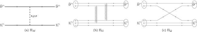
Figure 1. Feynman diagrams between ${\bar{D}}^{(* )}$ and ${{\rm{\Sigma }}}_{c}^{(* )}$ corresponding to : (a) the one-meson-exchange interaction ΠM, (b) the double-gluon-exchange interaction ΠG, and c) the light-quark-exchange interaction ΠQ. Here q denotes a light up/down quark.
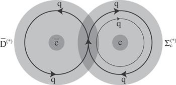
Figure 2. Possible binding mechanism induced by shared light quarks, described by the light-quark-exchange term ΠQ. Here q denotes a light up/down quark.
In this paper we shall systematically examine the Feynman diagrams corresponding to the ${\bar{D}}^{(* )}{{\rm{\Sigma }}}_{c}^{(* )}$, ${\bar{D}}^{(* )}{{\rm{\Lambda }}}_{c}$, ${D}^{(* )}{\bar{K}}^{* }$, and ${D}^{(* )}{\bar{D}}^{(* )}$ hadronic molecular states. We shall apply the method of QCD sum rules to investigate the light-quark-exchange term ΠQ, and study its contributions to these states. Based on the obtained results, we shall study the binding mechanism induced by shared light quarks. This mechanism is somewhat similar to the covalent bond in chemical molecules induced by shared electrons, so we call such hadronic molecules ‘covalent hadronic molecules'.
Based on the obtained results, we shall further propose a model-independent hypothesis: the light-quark-exchange interaction is attractive when the shared light quarks are totally antisymmetric so that they obey the Pauli principle. We shall apply this hypothesis to predict some possibly-existing covalent hadronic molecules. We shall also build a toy model to formulize this picture and estimate their binding energies. Our model has four parameters, which are fixed by considering the Pc/Pcs and the recently observed ${T}_{{cc}}^{+}$ [44, 45] as possible covalent hadronic molecules.
Take the X(3872) as another example. We shall find that the light-quark-exchange term ΠQ does not contribute to the ${D}^{(* )}{\bar{D}}^{(* )}$ molecules, suggesting the ${D}^{(* )}{\bar{D}}^{(* )}$ covalent hadronic molecules not to exist. However, there can still be the ${D}^{(* )}{\bar{D}}^{(* )}$ hadronic molecules induced by some other binding mechanisms, such as the one-meson-exchange interaction [2332]. Especially, the X(3872) can be interpreted as such a $D{\bar{D}}^{* }$ hadronic molecule, while it was suggested to be a compact tetraquark state in [4650], a conventional $c\bar{c}$ state in [51, 52], and the mixture of a $c\bar{c}$ state with the $D{\bar{D}}^{* }$ component in [53, 54].
This paper is organized as follows. In section 2 we systematically investigate correlation functions of the ${D}^{-}{{\rm{\Sigma }}}_{c}^{++}$, ${\bar{D}}^{0}{{\rm{\Sigma }}}_{c}^{+}$, I = 1/2 $\bar{D}{{\rm{\Sigma }}}_{c}$, and I = 3/2 $\bar{D}{{\rm{\Sigma }}}_{c}$ hadronic molecules. In section 3 we apply the method of QCD sum rules to investigate the light-quark-exchange term ΠQ, and study its contributions to these molecules. In section 4 we follow the same procedures and study the ${\bar{D}}^{* }{{\rm{\Sigma }}}_{c}/\bar{D}{{\rm{\Sigma }}}_{c}^{* }/{\bar{D}}^{* }{{\rm{\Sigma }}}_{c}^{* }$, ${\bar{D}}^{(* )}{{\rm{\Lambda }}}_{c}$, ${D}^{(* )}{\bar{K}}^{* }$, and ${D}^{(* )}{\bar{D}}^{(* )}$ hadronic molecules. Based on the obtained QCD sum rule results, we propose the above hypothesis in section 5, and predict more possibly-existing covalent hadronic molecules. In section 6 we build a toy model to formulize the covalent hadronic molecule picture, and the obtained results are summarized and discussed in section 7.

2. Correlation functions of ${D}^{-}{{\rm{\Sigma }}}_{c}^{++}/{\bar{D}}^{0}{{\rm{\Sigma }}}_{c}^{+}/\bar{D}{{\rm{\Sigma }}}_{c}$ molecules

In this section we investigate correlation functions of the ${D}^{-}{{\rm{\Sigma }}}_{c}^{++}$, ${\bar{D}}^{0}{{\rm{\Sigma }}}_{c}^{+}$, I = 1/2 $\bar{D}{{\rm{\Sigma }}}_{c}$, and I = 3/2 $\bar{D}{{\rm{\Sigma }}}_{c}$ hadronic molecular states.

2.1. ${D}^{-}{{\rm{\Sigma }}}_{c}^{++}$ correlation function

In this subsection we investigate the correlation function of the ${D}^{-}{{\rm{\Sigma }}}_{c}^{++}$ molecule. Firstly, we investigate the correlation functions of the D meson and the ${{\rm{\Sigma }}}_{c}^{++}$ baryon. Their corresponding interpolating currents are
$\begin{eqnarray}{J}^{{D}^{-}}(x)={\bar{c}}_{a}(x){\gamma }_{5}{d}_{a}(x),\end{eqnarray}$
$\begin{eqnarray}{J}^{{{\rm{\Sigma }}}_{c}^{++}}(x)=\displaystyle \frac{1}{\sqrt{2}}{\epsilon }^{{abc}}{u}_{a}^{{\rm{T}}}(x){\mathbb{C}}{\gamma }^{\mu }{u}_{b}(x){\gamma }_{\mu }{\gamma }_{5}{c}_{c}(x),\end{eqnarray}$
where ac are color indices; ${\mathbb{C}}={\rm{i}}{\gamma }_{2}{\gamma }_{0}$ is the charge-conjugation operator; the coefficient $1/\sqrt{2}$ is an isospin factor.
We write down two-point correlation functions of the D meson and the ${{\rm{\Sigma }}}_{c}^{++}$ baryon in the coordinate space:
$\begin{eqnarray}\begin{array}{rcl}{{\rm{\Pi }}}^{{D}^{-}}(x) & = & \langle 0| {\mathbb{T}}\left[{J}^{{D}^{-}}(x){J}^{{D}^{-},\dagger }(0)\right]| 0\rangle \\ & = & -{\bf{Tr}}\left[{{\bf{iS}}}_{q}^{{{aa}}^{{\prime} }}(x){\gamma }_{5}{{\bf{iS}}}_{c}^{{a}^{{\prime} }a}(-x){\gamma }_{5}\right],\end{array}\end{eqnarray}$
$\begin{eqnarray}\begin{array}{rcl}{{\rm{\Pi }}}^{{{\rm{\Sigma }}}_{c}^{++}}(x) & = & \langle 0| {\mathbb{T}}\left[{J}^{{{\rm{\Sigma }}}_{c}^{++}}(x){\bar{J}}^{{{\rm{\Sigma }}}_{c}^{++}}(0)\right]| 0\rangle \\ & = & {\epsilon }^{{abc}}{\epsilon }^{{a}^{{\prime} }{b}^{{\prime} }{c}^{{\prime} }}{\bf{Tr}}\left[{{\bf{iS}}}_{q}^{{{bb}}^{{\prime} }}(x){\gamma }^{{\mu }^{{\prime} }}{\mathbb{C}}{\left({{\bf{iS}}}_{q}^{{{aa}}^{{\prime} }}(x)\right)}^{{\rm{T}}}{\mathbb{C}}{\gamma }^{\mu }\right]\\ & & \times {\gamma }_{\mu }{\gamma }_{5}{{\bf{iS}}}_{c}^{{{cc}}^{{\prime} }}(x){\gamma }_{{\mu }^{{\prime} }}{\gamma }_{5}.\end{array}\end{eqnarray}$
Their corresponding Feynman diagrams are depicted in figures 3(a) and (b), respectively. In the present study we do not differentiate propagators of the light up and down quarks, and use ${{\bf{iS}}}_{q}^{{ab}}(x)={{\bf{iS}}}_{\mathrm{up}}^{{ab}}(x)={{\bf{iS}}}_{\mathrm{down}}^{{ab}}(x)$ to denote both of them in the coordinate space; besides, we use ${{\bf{iS}}}_{c}^{{ab}}(x)$ to denote the propagator of the heavy charm quark in the coordinate space:
$\begin{eqnarray}\begin{array}{rcl}{{\bf{iS}}}_{q}^{{ab}}(x) & = & \langle 0| {\mathbb{T}}\left[{u}^{a}(x){\bar{u}}^{b}(0)\right]| 0\rangle \\ & = & \langle 0| {\mathbb{T}}\left[{d}^{a}(x){\bar{d}}^{b}(0)\right]| 0\rangle ,\end{array}\end{eqnarray}$
$\begin{eqnarray}{{\bf{iS}}}_{c}^{{ab}}(x)=\langle 0| {\mathbb{T}}\left[{c}^{a}(x){\bar{c}}^{b}(0)\right]| 0\rangle .\end{eqnarray}$
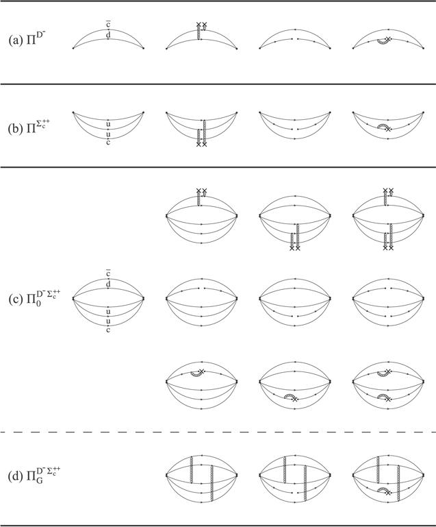
Figure 3. Feynman diagrams corresponding to: (a) ${{\rm{\Pi }}}^{{D}^{-}}(x)$, (b) ${{\rm{\Pi }}}^{{{\rm{\Sigma }}}_{c}^{++}}(x)$, (c) ${{\rm{\Pi }}}_{0}^{{D}^{-}{{\rm{\Sigma }}}_{c}^{++}}(x)$, and (d) ${{\rm{\Pi }}}_{G}^{{D}^{-}{{\rm{\Sigma }}}_{c}^{++}}(x)$. ${{\rm{\Pi }}}^{{D}^{-}}(x)$ and ${{\rm{\Pi }}}^{{{\rm{\Sigma }}}_{c}^{++}}(x)$ are correlation functions of the D meson and the ${{\rm{\Sigma }}}_{c}^{++}$ baryon, respectively. The correlation function of the ${D}^{-}{{\rm{\Sigma }}}_{c}^{++}$ molecule satisfies ${{\rm{\Pi }}}^{{D}^{-}{{\rm{\Sigma }}}_{c}^{++}}(x)={{\rm{\Pi }}}_{0}^{{D}^{-}{{\rm{\Sigma }}}_{c}^{++}}(x)+{{\rm{\Pi }}}_{G}^{{D}^{-}{{\rm{\Sigma }}}_{c}^{++}}(x)$ with ${{\rm{\Pi }}}_{0}^{{D}^{-}{{\rm{\Sigma }}}_{c}^{++}}(x)={{\rm{\Pi }}}^{{D}^{-}}(x)\times {{\rm{\Pi }}}^{{{\rm{\Sigma }}}_{c}^{++}}(x)$.
Then we put the D meson and the ${{\rm{\Sigma }}}_{c}^{++}$ baryon at the same location, and construct a composite current corresponding to the ${D}^{-}{{\rm{\Sigma }}}_{c}^{++}$ molecule,
$\begin{eqnarray}\begin{array}{rcl}{J}^{{D}^{-}{{\rm{\Sigma }}}_{c}^{++}}(x) & = & {J}^{{D}^{-}}(x)\times {J}^{{{\rm{\Sigma }}}_{c}^{++}}(x)\\ & = & [{\bar{c}}_{d}(x){\gamma }_{5}{d}_{d}(x)]\\ & & \times \displaystyle \frac{1}{\sqrt{2}}[{\epsilon }^{{abc}}{u}_{a}^{{\rm{T}}}(x){\mathbb{C}}{\gamma }^{\mu }{u}_{b}(x){\gamma }_{\mu }{\gamma }_{5}{c}_{c}(x)].\end{array}\end{eqnarray}$
Its correlation function in the coordinate space is
$\begin{eqnarray}\begin{array}{l}{{\rm{\Pi }}}^{{D}^{-}{{\rm{\Sigma }}}_{c}^{++}}(x)\\ \quad =\langle 0| {\mathbb{T}}\left[{J}^{{D}^{-}{{\rm{\Sigma }}}_{c}^{++}}(x){\bar{J}}^{{D}^{-}{{\rm{\Sigma }}}_{c}^{++}}(0)\right]| 0\rangle \\ \quad =-{\bf{Tr}}\left[{{\bf{iS}}}_{q}^{{{dd}}^{{\prime} }}(x){\gamma }_{5}{{\bf{iS}}}_{c}^{{d}^{{\prime} }d}(-x){\gamma }_{5}\right]\\ \quad \times {\epsilon }^{{abc}}{\epsilon }^{{a}^{{\prime} }{b}^{{\prime} }{c}^{{\prime} }}{\bf{Tr}}\left[{{\bf{iS}}}_{q}^{{{bb}}^{{\prime} }}(x){\gamma }^{{\mu }^{{\prime} }}{\mathbb{C}}{\left({{\bf{iS}}}_{q}^{{{aa}}^{{\prime} }}(x)\right)}^{{\rm{T}}}{\mathbb{C}}{\gamma }^{\mu }\right]\\ \quad \times {\gamma }_{\mu }{\gamma }_{5}{{\bf{iS}}}_{c}^{{{cc}}^{{\prime} }}(x){\gamma }_{{\mu }^{{\prime} }}{\gamma }_{5}\\ \quad ={{\rm{\Pi }}}_{0}^{{D}^{-}{{\rm{\Sigma }}}_{c}^{++}}(x)+{{\rm{\Pi }}}_{G}^{{D}^{-}{{\rm{\Sigma }}}_{c}^{++}}(x),\end{array}\end{eqnarray}$
where
$\begin{eqnarray}{{\rm{\Pi }}}_{0}^{{D}^{-}{{\rm{\Sigma }}}_{c}^{++}}(x)={{\rm{\Pi }}}^{{D}^{-}}(x)\times {{\rm{\Pi }}}^{{{\rm{\Sigma }}}_{c}^{++}}(x),\end{eqnarray}$
is the leading term contributed by non-correlated D and ${{\rm{\Sigma }}}_{c}^{++}$, and ${{\rm{\Pi }}}_{G}^{{D}^{-}{{\rm{\Sigma }}}_{c}^{++}}(x)$ describes the double-gluon-exchange interaction between them. Their corresponding Feynman diagrams are depicted in figures 3(c) and (d), respectively.
The double-gluon-exchange term ${{\rm{\Pi }}}_{G}^{{D}^{-}{{\rm{\Sigma }}}_{c}^{++}}(x)$ is at the ${ \mathcal O }({\alpha }_{s}^{2})$ order, and it is expected to be suppressed according to the OZI rule. In the present study we shall not pay much attention to it, while we shall investigate another more important term from the next subsection.

2.2. ${\bar{D}}^{0}{{\rm{\Sigma }}}_{c}^{+}$ correlation function

In this subsection we investigate the correlation function of the ${\bar{D}}^{0}{{\rm{\Sigma }}}_{c}^{+}$ molecule. The interpolating currents corresponding to the ${\bar{D}}^{0}$ meson, the ${{\rm{\Sigma }}}_{c}^{+}$ baryon, and the ${\bar{D}}^{0}{{\rm{\Sigma }}}_{c}^{+}$ molecule are
$\begin{eqnarray}{J}^{{\bar{D}}^{0}}(x)={\bar{c}}_{a}(x){\gamma }_{5}{u}_{a}(x),\end{eqnarray}$
$\begin{eqnarray}{J}^{{{\rm{\Sigma }}}_{c}^{+}}(x)={\epsilon }^{{abc}}{u}_{a}^{{\rm{T}}}(x){\mathbb{C}}{\gamma }^{\mu }{d}_{b}(x){\gamma }_{\mu }{\gamma }_{5}{c}_{c}(x),\end{eqnarray}$
$\begin{eqnarray}\begin{array}{rcl}{J}^{{\bar{D}}^{0}{{\rm{\Sigma }}}_{c}^{+}}(x) & = & {J}^{{\bar{D}}^{0}}(x)\times {J}^{{{\rm{\Sigma }}}_{c}^{+}}(x)\\ & = & [{\bar{c}}_{d}(x){\gamma }_{5}{u}_{d}(x)]\\ & & \times [{\epsilon }^{{abc}}{u}_{a}^{{\rm{T}}}(x){\mathbb{C}}{\gamma }^{\mu }{d}_{b}(x){\gamma }_{\mu }{\gamma }_{5}{c}_{c}(x)].\end{array}\end{eqnarray}$
Their correlation functions in the coordinate space are:
$\begin{eqnarray}{{\rm{\Pi }}}^{{\bar{D}}^{0}}(x)=-{\bf{Tr}}\left[{{\bf{iS}}}_{q}^{{{aa}}^{{\prime} }}(x){\gamma }_{5}{{\bf{iS}}}_{c}^{{a}^{{\prime} }a}(-x){\gamma }_{5}\right],\end{eqnarray}$
$\begin{eqnarray}\begin{array}{rcl}{{\rm{\Pi }}}^{{{\rm{\Sigma }}}_{c}^{+}}(x) & = & {\epsilon }^{{abc}}{\epsilon }^{{a}^{{\prime} }{b}^{{\prime} }{c}^{{\prime} }}{\bf{Tr}}\left[{{\bf{iS}}}_{q}^{{{bb}}^{{\prime} }}(x){\gamma }^{{\mu }^{{\prime} }}{\mathbb{C}}{\left({{\bf{iS}}}_{q}^{{{aa}}^{{\prime} }}(x)\right)}^{{\rm{T}}}{\mathbb{C}}{\gamma }^{\mu }\right]\\ & & \times {\gamma }_{\mu }{\gamma }_{5}{{\bf{iS}}}_{c}^{{{cc}}^{{\prime} }}(x){\gamma }_{{\mu }^{{\prime} }}{\gamma }_{5},\end{array}\end{eqnarray}$
$\begin{eqnarray}\begin{array}{l}{{\rm{\Pi }}}^{{\bar{D}}^{0}{{\rm{\Sigma }}}_{c}^{+}}(x)=-{\bf{Tr}}\left[{{\bf{iS}}}_{q}^{{{dd}}^{{\prime} }}(x){\gamma }_{5}{{\bf{iS}}}_{c}^{{d}^{{\prime} }d}(-x){\gamma }_{5}\right]\\ \quad \times {\epsilon }^{{abc}}{\epsilon }^{{a}^{{\prime} }{b}^{{\prime} }{c}^{{\prime} }}{\bf{Tr}}\left[{{\bf{iS}}}_{q}^{{{bb}}^{{\prime} }}(x){\gamma }^{{\mu }^{{\prime} }}{\mathbb{C}}{\left({{\bf{iS}}}_{q}^{{{aa}}^{{\prime} }}(x)\right)}^{{\rm{T}}}{\mathbb{C}}{\gamma }^{\mu }\right]\\ \quad \times {\gamma }_{\mu }{\gamma }_{5}{{\bf{iS}}}_{c}^{{{cc}}^{{\prime} }}(x){\gamma }_{{\mu }^{{\prime} }}{\gamma }_{5}\\ \quad +{\bf{Tr}}\left[{{\bf{iS}}}_{q}^{{{da}}^{{\prime} }}(x){\gamma }^{{\mu }^{{\prime} }}{\mathbb{C}}{\left({{\bf{iS}}}_{q}^{{{bb}}^{{\prime} }}(x)\right)}^{{\rm{T}}}{\mathbb{C}}{\gamma }^{\mu }{{\bf{iS}}}_{q}^{{{ad}}^{{\prime} }}(x){\gamma }_{5}{{\bf{iS}}}_{c}^{{d}^{{\prime} }d}(-x){\gamma }_{5}\right]\\ \quad \times {\gamma }_{\mu }{\gamma }_{5}{{\bf{iS}}}_{c}^{{{cc}}^{{\prime} }}(x){\gamma }_{{\mu }^{{\prime} }}{\gamma }_{5}\\ \quad ={{\rm{\Pi }}}_{0}^{{\bar{D}}^{0}{{\rm{\Sigma }}}_{c}^{+}}(x)+{{\rm{\Pi }}}_{G}^{{\bar{D}}^{0}{{\rm{\Sigma }}}_{c}^{+}}(x)+{{\rm{\Pi }}}_{Q}^{{\bar{D}}^{0}{{\rm{\Sigma }}}_{c}^{+}}(x).\end{array}\end{eqnarray}$
In the above expressions, ${{\rm{\Pi }}}^{{\bar{D}}^{0}}(x)$ and ${{\rm{\Pi }}}^{{{\rm{\Sigma }}}_{c}^{+}}(x)$ are correlation functions of ${\bar{D}}^{0}$ and ${{\rm{\Sigma }}}_{c}^{+}$, respective; ${{\rm{\Pi }}}_{0}^{{\bar{D}}^{0}{{\rm{\Sigma }}}_{c}^{+}}(x)\,={{\rm{\Pi }}}^{{\bar{D}}^{0}}(x)\times {{\rm{\Pi }}}^{{{\rm{\Sigma }}}_{c}^{+}}(x)$ is the leading term contributed by non-correlated ${\bar{D}}^{0}$ and ${{\rm{\Sigma }}}_{c}^{+}$, and ${{\rm{\Pi }}}_{G}^{{\bar{D}}^{0}{{\rm{\Sigma }}}_{c}^{+}}(x)$ describes the double-gluon-exchange interaction between them. Their corresponding Feynman diagrams are depicted in figures 4(a)–(d).
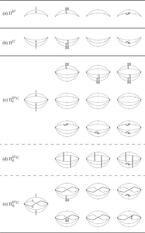
Figure 4. Feynman diagrams corresponding to: (a) ${{\rm{\Pi }}}^{{\bar{D}}^{0}}(x)$, (b) ${{\rm{\Pi }}}^{{{\rm{\Sigma }}}_{c}^{+}}(x)$, (c) ${{\rm{\Pi }}}_{0}^{{\bar{D}}^{0}{{\rm{\Sigma }}}_{c}^{+}}(x)$, (d) ${{\rm{\Pi }}}_{G}^{{\bar{D}}^{0}{{\rm{\Sigma }}}_{c}^{+}}(x)$, and (e) ${{\rm{\Pi }}}_{Q}^{{\bar{D}}^{0}{{\rm{\Sigma }}}_{c}^{+}}(x)$. ${{\rm{\Pi }}}^{{\bar{D}}^{0}}(x)$ and ${{\rm{\Pi }}}^{{{\rm{\Sigma }}}_{c}^{+}}(x)$ are correlation functions of the ${\bar{D}}^{0}$ meson and the ${{\rm{\Sigma }}}_{c}^{+}$ baryon, respectively. The correlation function of the ${\bar{D}}^{0}{{\rm{\Sigma }}}_{c}^{+}$ molecule satisfies ${{\rm{\Pi }}}^{{\bar{D}}^{0}{{\rm{\Sigma }}}_{c}^{+}}(x)={{\rm{\Pi }}}_{0}^{{\bar{D}}^{0}{{\rm{\Sigma }}}_{c}^{+}}(x)+{{\rm{\Pi }}}_{G}^{{\bar{D}}^{0}{{\rm{\Sigma }}}_{c}^{+}}(x)+{{\rm{\Pi }}}_{Q}^{{\bar{D}}^{0}{{\rm{\Sigma }}}_{c}^{+}}(x)$ with ${{\rm{\Pi }}}_{0}^{{\bar{D}}^{0}{{\rm{\Sigma }}}_{c}^{+}}(x)={{\rm{\Pi }}}^{{\bar{D}}^{0}}(x)\times {{\rm{\Pi }}}^{{{\rm{\Sigma }}}_{c}^{+}}(x)$.
Compared to the case of ${D}^{-}{{\rm{\Sigma }}}_{c}^{++}$, we find
$\begin{eqnarray}{{\rm{\Pi }}}^{{\bar{D}}^{0}}(x)={{\rm{\Pi }}}^{{D}^{-}}(x),\end{eqnarray}$
$\begin{eqnarray}{{\rm{\Pi }}}^{{{\rm{\Sigma }}}_{c}^{+}}(x)={{\rm{\Pi }}}^{{{\rm{\Sigma }}}_{c}^{++}}(x),\end{eqnarray}$
$\begin{eqnarray}{{\rm{\Pi }}}_{0}^{{\bar{D}}^{0}{{\rm{\Sigma }}}_{c}^{+}}(x)={{\rm{\Pi }}}_{0}^{{D}^{-}{{\rm{\Sigma }}}_{c}^{++}}(x),\end{eqnarray}$
$\begin{eqnarray}{{\rm{\Pi }}}_{G}^{{\bar{D}}^{0}{{\rm{\Sigma }}}_{c}^{+}}(x)={{\rm{\Pi }}}_{G}^{{D}^{-}{{\rm{\Sigma }}}_{c}^{++}}(x),\end{eqnarray}$
while there exists an extra term,
$\begin{eqnarray}\begin{array}{rcl}{{\rm{\Pi }}}_{Q}^{{\bar{D}}^{0}{{\rm{\Sigma }}}_{c}^{+}}(x) & = & {\bf{Tr}}\left[{{\bf{iS}}}_{q}^{{{da}}^{{\prime} }}(x){\gamma }^{{\mu }^{{\prime} }}{\mathbb{C}}{\left({{\bf{iS}}}_{q}^{{{bb}}^{{\prime} }}(x)\right)}^{{\rm{T}}}{\mathbb{C}}{\gamma }^{\mu }\right.\\ & & \times \left.{{\bf{iS}}}_{q}^{{{ad}}^{{\prime} }}(x){\gamma }_{5}{{\bf{iS}}}_{c}^{{d}^{{\prime} }d}(-x){\gamma }_{5}\right]\\ & & \times {\gamma }_{\mu }{\gamma }_{5}{{\bf{iS}}}_{c}^{{{cc}}^{{\prime} }}(x){\gamma }_{{\mu }^{{\prime} }}{\gamma }_{5}.\end{array}\end{eqnarray}$
Its corresponding Feynman diagrams are depicted in figure 4(e). This term describes the light-quark-exchange effect between ${\bar{D}}^{0}$ and ${{\rm{\Sigma }}}_{c}^{+}$, i.e. ${\bar{D}}^{0}$ and ${{\rm{\Sigma }}}_{c}^{+}$ are exchanging and so sharing two light up quarks. It can induce an interaction between ${\bar{D}}^{0}$ and ${{\rm{\Sigma }}}_{c}^{+}$, either attractive or repulsive. This term is color-unconfined, i.e. its contribution decreases as the distance between ${\bar{D}}^{0}$ and ${{\rm{\Sigma }}}_{c}^{+}$ increases; besides, the two exchanged/shared light quarks have the same color. We shall further study it numerically in section 3.3.

2.3. I = 1/2 $\bar{D}{{\rm{\Sigma }}}_{c}$ correlation function

In this subsection we investigate the correlation function of the I = 1/2 $\bar{D}{{\rm{\Sigma }}}_{c}$ molecule. Its corresponding interpolating current is
$\begin{eqnarray}{J}^{\bar{D}{{\rm{\Sigma }}}_{c}}(x)=\sqrt{\displaystyle \frac{1}{3}}{J}^{{\bar{D}}^{0}{{\rm{\Sigma }}}_{c}^{+}}(x)-\sqrt{\displaystyle \frac{2}{3}}{J}^{{D}^{-}{{\rm{\Sigma }}}_{c}^{++}}(x),\end{eqnarray}$
with the correlation function in the coordinate space
$\begin{eqnarray}\begin{array}{l}{{\rm{\Pi }}}^{\bar{D}{{\rm{\Sigma }}}_{c}}(x)=-{\bf{Tr}}\left[{{\bf{iS}}}_{q}^{{{dd}}^{{\prime} }}(x){\gamma }_{5}{{\bf{iS}}}_{c}^{{d}^{{\prime} }d}(-x){\gamma }_{5}\right]\\ \quad \times {\epsilon }^{{abc}}{\epsilon }^{{a}^{{\prime} }{b}^{{\prime} }{c}^{{\prime} }}{\bf{Tr}}\left[{{\bf{iS}}}_{q}^{{{bb}}^{{\prime} }}(x){\gamma }^{{\mu }^{{\prime} }}{\mathbb{C}}{\left({{\bf{iS}}}_{q}^{{{aa}}^{{\prime} }}(x)\right)}^{{\rm{T}}}{\mathbb{C}}{\gamma }^{\mu }\right]\\ \quad \times {\gamma }_{\mu }{\gamma }_{5}{{\bf{iS}}}_{c}^{{{cc}}^{{\prime} }}(x){\gamma }_{{\mu }^{{\prime} }}{\gamma }_{5}\\ \quad -{\bf{Tr}}\left[{{\bf{iS}}}_{q}^{{{da}}^{{\prime} }}(x){\gamma }^{{\mu }^{{\prime} }}{\mathbb{C}}{\left({{\bf{iS}}}_{q}^{{{bb}}^{{\prime} }}(x)\right)}^{{\rm{T}}}{\mathbb{C}}{\gamma }^{\mu }{{\bf{iS}}}_{q}^{{{ad}}^{{\prime} }}(x)\right.\\ \quad \times \left.{\gamma }_{5}{{\bf{iS}}}_{c}^{{d}^{{\prime} }d}(-x){\gamma }_{5}\right]{\gamma }_{\mu }{\gamma }_{5}{{\bf{iS}}}_{c}^{{{cc}}^{{\prime} }}(x){\gamma }_{{\mu }^{{\prime} }}{\gamma }_{5}\\ \quad ={{\rm{\Pi }}}_{0}^{\bar{D}{{\rm{\Sigma }}}_{c}}(x)+{{\rm{\Pi }}}_{G}^{\bar{D}{{\rm{\Sigma }}}_{c}}(x)+{{\rm{\Pi }}}_{Q}^{\bar{D}{{\rm{\Sigma }}}_{c}}(x).\end{array}\end{eqnarray}$
Compared to the case of ${\bar{D}}^{0}{{\rm{\Sigma }}}_{c}^{+}$ given in equation (15), only the terms ${{\rm{\Pi }}}_{Q}^{\bar{D}{{\rm{\Sigma }}}_{c}}(x)$ and ${{\rm{\Pi }}}_{Q}^{{\bar{D}}^{0}{{\rm{\Sigma }}}_{c}^{+}}(x)$ are different/opposite:
$\begin{eqnarray}{{\rm{\Pi }}}_{0}^{\bar{D}{{\rm{\Sigma }}}_{c}}(x)={{\rm{\Pi }}}_{0}^{{\bar{D}}^{0}{{\rm{\Sigma }}}_{c}^{+}}(x),\end{eqnarray}$
$\begin{eqnarray}{{\rm{\Pi }}}_{G}^{\bar{D}{{\rm{\Sigma }}}_{c}}(x)={{\rm{\Pi }}}_{G}^{{\bar{D}}^{0}{{\rm{\Sigma }}}_{c}^{+}}(x),\end{eqnarray}$
$\begin{eqnarray}{{\rm{\Pi }}}_{Q}^{\bar{D}{{\rm{\Sigma }}}_{c}}(x)=-{{\rm{\Pi }}}_{Q}^{{\bar{D}}^{0}{{\rm{\Sigma }}}_{c}^{+}}(x).\end{eqnarray}$
Accordingly, if the term ΠQ(x) induces a repulsive interaction to the ${\bar{D}}^{0}{{\rm{\Sigma }}}_{c}^{+}$ molecule, it would induce an attractive interaction to the I = 1/2 $\bar{D}{{\rm{\Sigma }}}_{c}$ molecule; and vice verse. We shall further study it numerically in section 3.1. For completeness, we explicitly list that the term ${{\rm{\Pi }}}_{Q}^{\bar{D}{{\rm{\Sigma }}}_{c}}(x)$ is contributed separately by:
$\begin{eqnarray}\begin{array}{l}\langle 0| {\mathbb{T}}\left[\sqrt{\displaystyle \frac{1}{3}}{J}^{{\bar{D}}^{0}{{\rm{\Sigma }}}_{c}^{+}}(x)\sqrt{\displaystyle \frac{1}{3}}{\bar{J}}^{{\bar{D}}^{0}{{\rm{\Sigma }}}_{c}^{+}}(0)\right]| 0\rangle \to -\displaystyle \frac{1}{3}{{\rm{\Pi }}}_{Q}^{\bar{D}{{\rm{\Sigma }}}_{c}}(x),\\ \quad \langle 0| {\mathbb{T}}\left[\sqrt{\displaystyle \frac{2}{3}}{J}^{{D}^{-}{{\rm{\Sigma }}}_{c}^{++}}(x)\sqrt{\displaystyle \frac{2}{3}}{\bar{J}}^{{D}^{-}{{\rm{\Sigma }}}_{c}^{++}}(0)\right]| 0\rangle \to 0,\\ \quad -\langle 0| {\mathbb{T}}\left[\displaystyle \frac{{J}^{{\bar{D}}^{0}{{\rm{\Sigma }}}_{c}^{+}}(x)}{\sqrt{3}}\sqrt{\displaystyle \frac{2}{3}}{\bar{J}}^{{D}^{-}{{\rm{\Sigma }}}_{c}^{++}}(0)\right]| 0\rangle \to \displaystyle \frac{2}{3}{{\rm{\Pi }}}_{Q}^{\bar{D}{{\rm{\Sigma }}}_{c}}(x),\\ \quad -\langle 0| {\mathbb{T}}\left[\sqrt{\displaystyle \frac{2}{3}}{J}^{{D}^{-}{{\rm{\Sigma }}}_{c}^{++}}(x)\displaystyle \frac{{\bar{J}}^{{\bar{D}}^{0}{{\rm{\Sigma }}}_{c}^{+}}(0)}{\sqrt{3}}\right]| 0\rangle \to \displaystyle \frac{2}{3}{{\rm{\Pi }}}_{Q}^{\bar{D}{{\rm{\Sigma }}}_{c}}(x).\end{array}\end{eqnarray}$

2.4. I = 3/2 $\bar{D}{{\rm{\Sigma }}}_{c}$ correlation function

For completeness, we investigate the correlation function of the I = 3/2 $\bar{D}{{\rm{\Sigma }}}_{c}$ molecule in this subsection. Its corresponding interpolating current is
$\begin{eqnarray}{J}_{I=3/2}^{\bar{D}{{\rm{\Sigma }}}_{c}}(x)=\sqrt{\displaystyle \frac{2}{3}}{J}^{{\bar{D}}^{0}{{\rm{\Sigma }}}_{c}^{+}}(x)+\sqrt{\displaystyle \frac{1}{3}}{J}^{{D}^{-}{{\rm{\Sigma }}}_{c}^{++}}(x),\end{eqnarray}$
with the correlation function to be
$\begin{eqnarray}{{\rm{\Pi }}}_{I=3/2}^{\bar{D}{{\rm{\Sigma }}}_{c}}(x)={{\rm{\Pi }}}_{0}^{\bar{D}{{\rm{\Sigma }}}_{c}}(x)+{{\rm{\Pi }}}_{G}^{\bar{D}{{\rm{\Sigma }}}_{c}}(x)-2{{\rm{\Pi }}}_{Q}^{\bar{D}{{\rm{\Sigma }}}_{c}}(x).\end{eqnarray}$
In the above expression ${{\rm{\Pi }}}_{0}^{\bar{D}{{\rm{\Sigma }}}_{c}}(x)$, ${{\rm{\Pi }}}_{G}^{\bar{D}{{\rm{\Sigma }}}_{c}}(x)$, and ${{\rm{\Pi }}}_{Q}^{\bar{D}{{\rm{\Sigma }}}_{c}}(x)$ are taken from the I = 1/2 $\bar{D}{{\rm{\Sigma }}}_{c}$ molecule.
Compared to equation (22), if the term ΠQ(x) induces an attractive interaction to the I = 1/2 $\bar{D}{{\rm{\Sigma }}}_{c}$ molecule, it would induce a repulsive interaction to the I = 3/2 $\bar{D}{{\rm{\Sigma }}}_{c}$ molecule; and vice verse.

3. QCD sum rule studies of ${D}^{-}{{\rm{\Sigma }}}_{c}^{++}/{\bar{D}}^{0}{{\rm{\Sigma }}}_{c}^{+}/\bar{D}{{\rm{\Sigma }}}_{c}$ molecules

In this section we apply the method of QCD sum rules [55, 56] to investigate the light-quark-exchange term ΠQ(x), and study its contributions to the ${D}^{-}{{\rm{\Sigma }}}_{c}^{++}$, ${\bar{D}}^{0}{{\rm{\Sigma }}}_{c}^{+}$, I = 1/2 $\bar{D}{{\rm{\Sigma }}}_{c}$, and I = 3/2 $\bar{D}{{\rm{\Sigma }}}_{c}$ hadronic molecular states.
In QCD sum rule analyses we consider the two-point correlation function in the momentum space:
$\begin{eqnarray}\begin{array}{rcl}{\rm{\Pi }}({q}^{2}) & = & {\rm{i}}\displaystyle \int {{\rm{d}}}^{4}x{{\rm{e}}}^{{\rm{i}}{qx}}\langle 0| {\mathbb{T}}\left[J(x)\bar{J}(0)\right]| 0\rangle \\ & = & {\rm{i}}\displaystyle \int {{\rm{d}}}^{4}x{{\rm{e}}}^{{\rm{i}}{qx}}\,{\rm{\Pi }}(x),\end{array}\end{eqnarray}$
where J(x) is an interpolating current. We generally assume it to be a composite current, coupling to the molecular state $X\equiv \left|{YZ}\right\rangle $ through
$\begin{eqnarray}\langle 0| J| X\rangle ={f}_{X}{u}_{X}.\end{eqnarray}$
We write Π(q2) in the form of dispersion relation as
$\begin{eqnarray}{\rm{\Pi }}({q}^{2})={\int }_{{s}_{\lt }}^{\infty }\displaystyle \frac{\rho (s)}{s-{q}^{2}-{\rm{i}}\varepsilon }{\rm{d}}s,\end{eqnarray}$
where ${s}_{\lt }=4{m}_{c}^{2}$ is the physical threshold and $\rho (s)\equiv \mathrm{Im}{\rm{\Pi }}(s)/\pi $ is the spectral density.
At the quark-gluon level we calculate Π(q2) using the method of operator product expansion (OPE) up to certain order. According to equations (8), (15), (22), and (28), we further separate it into
$\begin{eqnarray}{\rm{\Pi }}({q}^{2})\approx {{\rm{\Pi }}}_{0}({q}^{2})+{{\rm{\Pi }}}_{Q}({q}^{2}),\end{eqnarray}$
and define their imaginary parts to be ρ0(s) and ρQ(s). Here we have omitted the other term ΠG(q2), since the light-quark-exchange term ΠQ(q2) is much larger.
At the hadron level we evaluate the spectral density by inserting intermediate hadron states ${\sum }_{n}\left|n\rangle \langle n\right|$:
$\begin{eqnarray}\begin{array}{rcl}\rho (s) & = & \sum _{n}\delta (s-{M}_{n}^{2})\langle 0| J| n\rangle \langle n| \bar{J}| 0\rangle \\ & = & {f}_{X}^{2}\delta (s-{M}_{X}^{2})+\mathrm{continuum},\end{array}\end{eqnarray}$
where we have adopted a parametrization of one pole dominance for the ground state X together with a continuum contribution.
Given $X\equiv \left|{YZ}\right\rangle $ to be a molecular state, its mass MX can be expanded as
$\begin{eqnarray}\begin{array}{rcl}{M}_{X} & = & {M}_{Y}+{M}_{Z}+{\rm{\Delta }}M\\ & \equiv & {M}_{0}+{\rm{\Delta }}M.\end{array}\end{eqnarray}$
Then we insert equation (33) into (31), and expand it as
$\begin{eqnarray}\begin{array}{rcl}{\rm{\Pi }}({q}^{2}) & = & \displaystyle \frac{{f}_{X}^{2}}{{M}_{X}^{2}-{q}^{2}}+\cdots \\ & \approx & \displaystyle \frac{{f}_{X}^{2}}{{M}_{0}^{2}-{q}^{2}}-\displaystyle \frac{2{M}_{0}{f}_{X}^{2}}{{\left({M}_{0}^{2}-{q}^{2}\right)}^{2}}{\rm{\Delta }}M+\cdots .\end{array}\end{eqnarray}$
The former term is contributed by the non-correlated Y and Z, and the latter term is contributed by their interactions. Compared to equation (32), we further obtain:
$\begin{eqnarray}{{\rm{\Pi }}}_{0}({q}^{2})=\displaystyle \frac{{f}_{X}^{2}}{{M}_{0}^{2}-{q}^{2}}+\cdots ,\end{eqnarray}$
$\begin{eqnarray}{{\rm{\Pi }}}_{Q}({q}^{2})=-\displaystyle \frac{2{M}_{0}{f}_{X}^{2}}{{\left({M}_{0}^{2}-{q}^{2}\right)}^{2}}{\rm{\Delta }}M+\cdots .\end{eqnarray}$
We perform the Borel transformation to the above correlation functions at both hadron and quark-gluon levels. After assuming contributions from the continuum to be approximated by the OPE spectral densities ρ0(s) and ρQ(s) above a threshold value s0, we arrive at two sum rule equations:
$\begin{eqnarray}\begin{array}{l}{f}_{X}^{2}{{\rm{e}}}^{-{M}_{0}^{2}/{M}_{B}^{2}}={{\rm{\Pi }}}_{0}({M}_{B}^{2},{s}_{0})\\ \quad ={\displaystyle \int }_{{s}_{\lt }}^{{s}_{0}}{{\rm{e}}}^{-s/{M}_{B}^{2}}{\rho }_{0}(s){\rm{d}}s,\end{array}\end{eqnarray}$
$\begin{eqnarray}\begin{array}{l}-\displaystyle \frac{2{M}_{0}{f}_{X}^{2}}{{M}_{B}^{2}}{\rm{\Delta }}M{{\rm{e}}}^{-{M}_{0}^{2}/{M}_{B}^{2}}={{\rm{\Pi }}}_{Q}({M}_{B}^{2},{s}_{0})\\ \quad ={\displaystyle \int }_{{s}_{\lt }}^{{s}_{0}}{{\rm{e}}}^{-s/{M}_{B}^{2}}{\rho }_{Q}(s){\rm{d}}s.\end{array}\end{eqnarray}$
There are two free parameters in equations (38) and (39): the Borel mass MB and the threshold value s0. Differentiating equation (38) with respect to $1/{M}_{B}^{2}$, we obtain
$\begin{eqnarray}{M}_{0}^{2}=\displaystyle \frac{{\int }_{{s}_{\lt }}^{{s}_{0}}{{\rm{e}}}^{-s/{M}_{B}^{2}}s\rho (s){\rm{d}}s}{{\int }_{{s}_{\lt }}^{{s}_{0}}{{\rm{e}}}^{-s/{M}_{B}^{2}}\rho (s){\rm{d}}s}.\end{eqnarray}$
Given M0 = MY + MZ, this equation can be used to relate MB and s0, so that there is only one free parameter left.
Dividing equation (39) by (38), we obtain
$\begin{eqnarray}-\displaystyle \frac{2{M}_{0}}{{M}_{B}^{2}}{\rm{\Delta }}M=\displaystyle \frac{{{\rm{\Pi }}}_{Q}}{{{\rm{\Pi }}}_{0}}=\displaystyle \frac{{\int }_{{s}_{\lt }}^{{s}_{0}}{{\rm{e}}}^{-s/{M}_{B}^{2}}{\rho }_{Q}(s){\rm{d}}s}{{\int }_{{s}_{\lt }}^{{s}_{0}}{{\rm{e}}}^{-s/{M}_{B}^{2}}{\rho }_{0}(s){\rm{d}}s}.\end{eqnarray}$
This equation can be used to calculate ΔM.
We shall use equation (41) to study contributions of the term ΠQ(x) to the ${D}^{-}{{\rm{\Sigma }}}_{c}^{++}$, ${\bar{D}}^{0}{{\rm{\Sigma }}}_{c}^{+}$, I = 1/2 $\bar{D}{{\rm{\Sigma }}}_{c}$, and I = 3/2 $\bar{D}{{\rm{\Sigma }}}_{c}$ hadronic molecular states, separately in the following subsections. Before doing this, we note that ΔM is actually not the binding energy, but relates to some potential V(r) between Y and Z induced by exchanged/shared light quarks. We use the I = 1/2 $\bar{D}{{\rm{\Sigma }}}_{c}$ hadronic molecular state as an example to qualitatively discuss this. After transforming the local current ${J}^{\bar{D}{{\rm{\Sigma }}}_{c}}(x)$ defined in equation (21) into its non-local form:
$\begin{eqnarray}\begin{array}{l}{J}^{\bar{D}{{\rm{\Sigma }}}_{c}}(x,y)\\ \quad =\sqrt{\displaystyle \frac{1}{3}}{J}^{{\bar{D}}^{0}{{\rm{\Sigma }}}_{c}^{+}}(x,y)-\sqrt{\displaystyle \frac{2}{3}}{J}^{{D}^{-}{{\rm{\Sigma }}}_{c}^{++}}(x,y)\\ \quad =\sqrt{\displaystyle \frac{1}{3}}{J}^{{\bar{D}}^{0}}(x){J}^{{{\rm{\Sigma }}}_{c}^{+}}(y)-\sqrt{\displaystyle \frac{2}{3}}{J}^{{D}^{-}}(x){J}^{{{\rm{\Sigma }}}_{c}^{++}}(y),\end{array}\end{eqnarray}$
we calculate its non-local correlation function in the coordinate space to be:
$\begin{eqnarray}\begin{array}{l}{{\rm{\Pi }}}^{\bar{D}{{\rm{\Sigma }}}_{c}}(x,y;{x}^{{\prime} },{y}^{{\prime} })\equiv \langle 0| {\mathbb{T}}\left[{J}^{\bar{D}{{\rm{\Sigma }}}_{c}}(x,y){\bar{J}}^{\bar{D}{{\rm{\Sigma }}}_{c}}({x}^{{\prime} },{y}^{{\prime} })\right]| 0\rangle \\ \quad =-{\bf{Tr}}\left[{{\bf{iS}}}_{q}^{{{dd}}^{{\prime} }}({\rm{\Delta }}x){\gamma }_{5}{{\bf{iS}}}_{c}^{{d}^{{\prime} }d}(-{\rm{\Delta }}x){\gamma }_{5}\right]\\ \quad \times {\epsilon }^{{abc}}{\epsilon }^{{a}^{{\prime} }{b}^{{\prime} }{c}^{{\prime} }}{\bf{Tr}}\left[{{\bf{iS}}}_{q}^{{{bb}}^{{\prime} }}({\rm{\Delta }}x){\gamma }^{{\mu }^{{\prime} }}{\mathbb{C}}{\left({{\bf{iS}}}_{q}^{{{aa}}^{{\prime} }}({\rm{\Delta }}x)\right)}^{{\rm{T}}}{\mathbb{C}}{\gamma }^{\mu }\right]\\ \quad \times {\gamma }_{\mu }{\gamma }_{5}{{\bf{iS}}}_{c}^{{{cc}}^{{\prime} }}({\rm{\Delta }}x){\gamma }_{{\mu }^{{\prime} }}{\gamma }_{5}\\ \quad -{\bf{Tr}}\left[{{\bf{iS}}}_{q}^{{{da}}^{{\prime} }}({\rm{\Delta }}x-r){\gamma }^{{\mu }^{{\prime} }}{\mathbb{C}}{\left({{\bf{iS}}}_{q}^{{{bb}}^{{\prime} }}({\rm{\Delta }}x)\right)}^{{\rm{T}}}{\mathbb{C}}{\gamma }^{\mu }{{\bf{iS}}}_{q}^{{{ad}}^{{\prime} }}\right.\\ \quad \times \left.({\rm{\Delta }}x+r){\gamma }_{5}{{\bf{iS}}}_{c}^{{d}^{{\prime} }d}(-{\rm{\Delta }}x){\gamma }_{5}\right]\\ \quad \times {\gamma }_{\mu }{\gamma }_{5}{{\bf{iS}}}_{c}^{{{cc}}^{{\prime} }}({\rm{\Delta }}x){\gamma }_{{\mu }^{{\prime} }}{\gamma }_{5}\\ \quad ={{\rm{\Pi }}}_{0}^{\bar{D}{{\rm{\Sigma }}}_{c}}({\rm{\Delta }}x)+{{\rm{\Pi }}}_{G}^{\bar{D}{{\rm{\Sigma }}}_{c}}({\rm{\Delta }}x,r)+{{\rm{\Pi }}}_{Q}^{\bar{D}{{\rm{\Sigma }}}_{c}}({\rm{\Delta }}x,r).\end{array}\end{eqnarray}$
In the above expression we have assumed that $y-{y}^{{\prime} }=x\,-{x}^{{\prime} }={\rm{\Delta }}x$ and $y-x={y}^{{\prime} }-{x}^{{\prime} }=r$. The leading term ${{\rm{\Pi }}}_{0}^{\bar{D}{{\rm{\Sigma }}}_{c}}({\rm{\Delta }}x)$ does not change with the parameter r, while the light-quark-exchange term ${{\rm{\Pi }}}_{Q}^{\bar{D}{{\rm{\Sigma }}}_{c}}({\rm{\Delta }}x,r)$ decreases as ∣r∣ → ∞. Accordingly, we arrive at:

Because we are using local currents in QCD sum rule analyses,

$\begin{eqnarray}V(| r| =0)={\rm{\Delta }}M.\end{eqnarray}$

Because the term ΠQ(x) is color-unconfined, its contribution decreases as r increases:

$\begin{eqnarray}V(| r| \to \infty )\to 0.\end{eqnarray}$

We may build a model and use the light-quark-exchange potential V(r) to derive the binding energy of X, but this will not be done in the present study. Other than this, we shall calculate ΔM and qualitatively study several hadronic molecules possibly bound by this potential, through which we shall propose a model-independent hypothesis for such molecules.
The binding mechanism induced by the light-quark-exchange potential V(r) is somewhat similar to the covalent bond in chemical molecules induced by shared electrons, so we call such hadronic molecules ‘covalent hadronic molecules'.

3.1. I = 1/2 $\bar{D}{{\rm{\Sigma }}}_{c}$ sum rules

In this subsection we apply QCD sum rules to study the I = 1/2 $\bar{D}{{\rm{\Sigma }}}_{c}$ molecule. We have calculated its correlation function at the leading order of αs and up to the D(imension) = 10 terms, including the perturbative term, the quark condensate $\langle \bar{q}q\rangle $, the gluon condensate $\langle {g}_{s}^{2}{GG}\rangle $, the quark-gluon mixed condensate $\langle {g}_{s}\bar{q}\sigma {Gq}\rangle $, and their combinations $\langle \bar{q}q{\rangle }^{2}$, $\langle \bar{q}q\rangle \langle {g}_{s}\bar{q}\sigma {Gq}\rangle $, $\langle \bar{q}q{\rangle }^{3}$, and $\langle {g}_{s}\bar{q}\sigma {Gq}{\rangle }^{2}$. The extracted spectral density
$\begin{eqnarray}{\rho }^{\bar{D}{{\rm{\Sigma }}}_{c}}(s)={\rho }_{0}^{\bar{D}{{\rm{\Sigma }}}_{c}}(s)+{\rho }_{Q}^{\bar{D}{{\rm{\Sigma }}}_{c}}(s),\end{eqnarray}$
is given in appendix A.
To perform numerical analyses, we use the following values for various QCD sum rule parameters in the present study [2, 5765]:
$\begin{eqnarray}\begin{array}{rcl}{m}_{s} & = & {96}_{-4}^{+8}{\rm{MeV}},\\ {m}_{c} & = & {1.275}_{-0.035}^{+0.025}\,{\rm{GeV}},\\ \langle \bar{q}q\rangle & = & -{\left(0.240\pm 0.010\right)}^{3}\,{{\rm{GeV}}}^{3},\\ \langle \bar{s}s\rangle & = & (0.8\pm 0.1)\times \langle \bar{q}q\rangle ,\\ \langle {g}_{s}^{2}{GG}\rangle & = & 0.48\pm 0.14\,{{\rm{GeV}}}^{4},\\ \langle {g}_{s}\bar{q}\sigma {Gq}\rangle & = & -{M}_{0}^{2}\times \langle \bar{q}q\rangle ,\\ \langle {g}_{s}\bar{s}\sigma {Gs}\rangle & = & -{M}_{0}^{2}\times \langle \bar{s}s\rangle ,\\ {M}_{0}^{2} & = & 0.8\pm 0.2\,{{\rm{GeV}}}^{2},\end{array}\end{eqnarray}$
where the running mass in the $\overline{{MS}}$ scheme is used for the charm quark.
There are two free parameters in equations (38) and (39): the Borel mass MB and the threshold value s0. We use equation (40) to constrain them by setting [2]:
$\begin{eqnarray}\begin{array}{rcl}{M}_{0}^{\bar{D}{{\rm{\Sigma }}}_{c}} & = & \displaystyle \frac{1}{3}\times \left({M}_{{\bar{D}}^{0}}+{M}_{{{\rm{\Sigma }}}_{c}^{+}}\right)+\displaystyle \frac{2}{3}\times \left({M}_{{D}^{-}}+{M}_{{{\rm{\Sigma }}}_{c}^{++}}\right)\\ & = & 4321.66\,\mathrm{MeV}.\end{array}\end{eqnarray}$
The derived relation between MB and s0 is depicted in figure 5, which will be used in the following calculations.
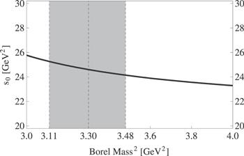
Figure 5. Relation between the Borel mass MB and the threshold value s0, constrained by equation (40).
There are two criteria to constrain the Borel mass MB. The first criterion is to ensure the convergence of OPE series, by requiring the D = 10 terms ${m}_{c}\langle \bar{q}q{\rangle }^{3}$ and $\langle {g}_{s}\bar{q}\sigma {Gq}{\rangle }^{2}$ to be less than 15%:
$\begin{eqnarray}{\rm{Convergence}}\equiv \left|\displaystyle \frac{{{\rm{\Pi }}}^{D=10}(\infty ,{M}_{B})}{{\rm{\Pi }}(\infty ,{M}_{B})}\right|\leqslant 15 \% .\end{eqnarray}$
This criterion determines the lower limit of MB. As shown in figure 6 using the solid curve, we find it to be ${\left({M}_{B}^{\min }\right)}^{2}\,=\,3.11$ GeV2.
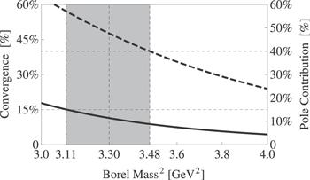
Figure 6. Convergence (solid) and Pole-Contribution (dashed) as functions of the Borel mass MB.
The second criterion is to ensure the validity of one-pole parametrization, by requiring the pole contribution to be larger than 40%:
$\begin{eqnarray}{\rm{Pole-Contribution}}\equiv \displaystyle \frac{{\rm{\Pi }}({s}_{0}({M}_{B}),{M}_{B})}{{\rm{\Pi }}(\infty ,{M}_{B})}\geqslant 40 \% .\end{eqnarray}$
This determines the upper limit of MB. As shown in figure 6 using the dashed curve, we find it to be ${\left({M}_{B}^{\max }\right)}^{2}\,=\,3.48$ GeV2.
Altogether we extract the working region of MB to be 3.11 GeV${}^{2}\lt {M}_{B}^{2}\lt 3.48$ GeV2, where we use equation (41) to calculate the mass correction to be
$\begin{eqnarray}{\rm{\Delta }}{M}_{I=1/2,J=1/2}^{\bar{D}{{\rm{\Sigma }}}_{c}}=-95\,\mathrm{MeV}.\end{eqnarray}$
We show its variation in figure 7 with respect to the Borel mass MB. It is shown in a broader region 3.0 GeV${}^{2}\leqslant {M}_{B}^{2}\leqslant 4.0$ GeV2, and we find it quite stable inside the above Borel window.
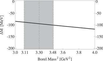
Figure 7. The mass correction ${\rm{\Delta }}{M}_{I=1/2,J=1/2}^{\bar{D}{{\rm{\Sigma }}}_{c}}$ as a function of the Borel mass MB.
The mass correction ${\rm{\Delta }}{M}_{I=1/2,J=1/2}^{\bar{D}{{\rm{\Sigma }}}_{c}}$ given in equation (51) is negative, suggesting the light-quark-exchange potential ${V}_{I=1/2,J=1/2}^{\bar{D}{{\rm{\Sigma }}}_{c}}(r)$ to be attractive, so there can be the $\bar{D}{{\rm{\Sigma }}}_{c}$ covalent molecule of I = 1/2 and J = 1/2.

3.2. ${D}^{-}{{\rm{\Sigma }}}_{c}^{++}$ sum rules

As shown in equation (8), the light-quark-exchange term ΠQ(x) does not contribute to the correlation function of the ${D}^{-}{{\rm{\Sigma }}}_{c}^{++}$ molecule, so the ${D}^{-}{{\rm{\Sigma }}}_{c}^{++}$ covalent molecule does not exist.

3.3. ${\bar{D}}^{0}{{\rm{\Sigma }}}_{c}^{+}$ sum rules

We follow section 3.1 to study the ${\bar{D}}^{0}{{\rm{\Sigma }}}_{c}^{+}$ molecule, and calculate its mass correction to be
$\begin{eqnarray}{\rm{\Delta }}{M}_{J=1/2}^{{\bar{D}}^{0}{{\rm{\Sigma }}}_{c}^{+}}\approx -{\rm{\Delta }}{M}_{I=1/2,J=1/2}^{\bar{D}{{\rm{\Sigma }}}_{c}}=95\,\mathrm{MeV}.\end{eqnarray}$
This result suggests ${V}_{J=1/2}^{{\bar{D}}^{0}{{\rm{\Sigma }}}_{c}^{+}}(r)$ to be repulsive, so the ${\bar{D}}^{0}{{\rm{\Sigma }}}_{c}^{+}$ covalent molecule does not exist.

3.4. I = 3/2 $\bar{D}{{\rm{\Sigma }}}_{c}$ sum rules

We follow section 3.1 to study the I = 3/2 $\bar{D}{{\rm{\Sigma }}}_{c}$ molecule, and calculate its mass correction to be
$\begin{eqnarray}{\rm{\Delta }}{M}_{I=3/2,J=1/2}^{\bar{D}{{\rm{\Sigma }}}_{c}}\approx -2{\rm{\Delta }}{M}_{I=1/2,J=1/2}^{\bar{D}{{\rm{\Sigma }}}_{c}}=190\,\mathrm{MeV}.\end{eqnarray}$
This result suggests ${V}_{I=3/2,J=1/2}^{\bar{D}{{\rm{\Sigma }}}_{c}}(r)$ to be repulsive, so the $\bar{D}{{\rm{\Sigma }}}_{c}$ covalent molecule of I = 3/2 and J = 1/2 does not exist.

4. More hadronic molecules

In this section we follow the procedures used in section 3.1 and study more possibly-existing covalent hadronic molecules. We shall investigate the ${\bar{D}}^{* }{{\rm{\Sigma }}}_{c}/\bar{D}{{\rm{\Sigma }}}_{c}^{* }/{\bar{D}}^{* }{{\rm{\Sigma }}}_{c}^{* }$ molecules, the ${\bar{D}}^{(* )}{{\rm{\Lambda }}}_{c}$ molecules, the ${D}^{(* )}{\bar{K}}^{* }$ molecules, and the ${D}^{(* )}{\bar{D}}^{(* )}$ molecules, separately in the following subsections.

4.1. ${\bar{D}}^{* }{{\rm{\Sigma }}}_{c}/\bar{D}{{\rm{\Sigma }}}_{c}^{* }/{\bar{D}}^{* }{{\rm{\Sigma }}}_{c}^{* }$ molecules

In this subsection we investigate the light-quark-exchange term ΠQ(x) and study its contributions to the ${\bar{D}}^{* }{{\rm{\Sigma }}}_{c}/\bar{D}{{\rm{\Sigma }}}_{c}^{* }/{\bar{D}}^{* }{{\rm{\Sigma }}}_{c}^{* }$ molecules.
The current corresponding to the ${\bar{D}}^{* }{{\rm{\Sigma }}}_{c}$ molecule is
$\begin{eqnarray}\begin{array}{l}{J}_{\alpha }^{{\bar{D}}^{* }{{\rm{\Sigma }}}_{c}}(x)={J}_{\alpha }^{{\bar{D}}^{* }}(x)\times {J}^{{{\rm{\Sigma }}}_{c}}(x)\\ \quad =[{\bar{c}}_{d}(x){\gamma }_{\alpha }{q}_{d}(x)]\times [{\epsilon }^{{abc}}{q}_{a}^{{\rm{T}}}(x){\mathbb{C}}{\gamma }^{\mu }{q}_{b}(x){\gamma }_{\mu }{\gamma }_{5}{c}_{c}(x)].\end{array}\end{eqnarray}$
Its correlation function is
$\begin{eqnarray}\begin{array}{l}{{\rm{\Pi }}}_{\alpha \beta }^{{\bar{D}}^{* }{{\rm{\Sigma }}}_{c}}({q}^{2})\\ \quad ={\rm{i}}\displaystyle \int {{\rm{d}}}^{4}x{{\rm{e}}}^{{\rm{i}}{qx}}\langle 0| {\mathbb{T}}\left[{J}_{\alpha }^{{\bar{D}}^{* }{{\rm{\Sigma }}}_{c}}(x){\bar{J}}_{\beta }^{{\bar{D}}^{* }{{\rm{\Sigma }}}_{c}}(0)\right]| 0\rangle \\ \quad ={{ \mathcal G }}_{\alpha \beta }^{3/2}({q}^{2})\,{{\rm{\Pi }}}_{J=3/2}^{{\bar{D}}^{* }{{\rm{\Sigma }}}_{c}}\left({q}^{2}\right)+{{ \mathcal G }}_{\alpha \beta }^{1/2}({q}^{2})\,{{\rm{\Pi }}}_{J=1/2}^{{\bar{D}}^{* }{{\rm{\Sigma }}}_{c}}\left({q}^{2}\right),\end{array}\end{eqnarray}$
where ${{\rm{\Pi }}}_{J=3/2}^{{\bar{D}}^{* }{{\rm{\Sigma }}}_{c}}\left({q}^{2}\right)$ and ${{\rm{\Pi }}}_{J=1/2}^{{\bar{D}}^{* }{{\rm{\Sigma }}}_{c}}\left({q}^{2}\right)$ are contributed by the spin-3/2 and spin-1/2 components, respectively. ${{ \mathcal G }}_{\alpha \beta }^{3/2}\left({q}^{2}\right)$ and ${{ \mathcal G }}_{\alpha \beta }^{1/2}\left({q}^{2}\right)$ are coefficients of the spin-3/2 and spin-1/2 propagators, respectively:
$\begin{eqnarray}\begin{array}{rcl}{{ \mathcal G }}_{\alpha \beta }^{3/2}({q}^{2}) & = & \left({g}_{\alpha \beta }-\displaystyle \frac{{\gamma }_{\alpha }{\gamma }_{\beta }}{3}-\displaystyle \frac{{q}_{\alpha }{\gamma }_{\beta }-{q}_{\beta }{\gamma }_{\alpha }}{3M}-\displaystyle \frac{2{q}_{\alpha }{q}_{\beta }}{3{M}^{2}}\right)\\ & & \times (q/\,+M),\end{array}\end{eqnarray}$
$\begin{eqnarray}{{ \mathcal G }}_{\alpha \beta }^{1/2}(q)={q}_{\alpha }{q}_{\beta }\times (q/\,+M).\end{eqnarray}$
In the present study we have only calculated the terms proportional to the Lorentz coefficient gαβ, so we can only extract the mass correction to the spin-3/2 ${\bar{D}}^{* }{{\rm{\Sigma }}}_{c}$ molecule. We find it negative for the I = 1/2 one:
$\begin{eqnarray}{\rm{\Delta }}{M}_{I=1/2,J=3/2}^{{\bar{D}}^{* }{{\rm{\Sigma }}}_{c}}=-89\,\mathrm{MeV}.\end{eqnarray}$
This result suggests ${V}_{I=1/2,J=3/2}^{{\bar{D}}^{* }{{\rm{\Sigma }}}_{c}}(r)$ to be attractive, so there can be the ${\bar{D}}^{* }{{\rm{\Sigma }}}_{c}$ covalent molecule of I = 1/2 and J = 3/2.
Similarly, we use the current
$\begin{eqnarray}\begin{array}{l}{J}_{\alpha }^{\bar{D}{{\rm{\Sigma }}}_{c}^{* }}(x)={J}^{\bar{D}}(x)\times {J}_{\alpha }^{{{\rm{\Sigma }}}_{c}^{* }}(x)\\ \quad =[{\bar{c}}_{d}(x){\gamma }_{5}{q}_{d}(x)]\times [{\epsilon }^{{abc}}{q}_{a}^{{\rm{T}}}(x){\mathbb{C}}{\gamma }^{\mu }{q}_{b}(x){P}_{\alpha \mu }^{3/2}{c}_{c}(x)],\end{array}\end{eqnarray}$
to perform QCD sum rule analyses and study the $\bar{D}{{\rm{\Sigma }}}_{c}^{* }$ molecule. Here ${P}_{\alpha \mu }^{3/2}$ is the spin-3/2 projection operator
$\begin{eqnarray}{P}_{\alpha \mu }^{3/2}={g}_{\alpha \mu }-\displaystyle \frac{1}{4}{\gamma }_{\alpha }{\gamma }_{\mu }.\end{eqnarray}$
We calculate its mass correction to be
$\begin{eqnarray}{\rm{\Delta }}{M}_{I=1/2,J=3/2}^{\bar{D}{{\rm{\Sigma }}}_{c}^{* }}=-86\,\mathrm{MeV}.\end{eqnarray}$
This result suggests ${V}_{I=1/2,J=3/2}^{\bar{D}{{\rm{\Sigma }}}_{c}^{* }}(r)$ to be attractive, so there can be the $\bar{D}{{\rm{\Sigma }}}_{c}^{* }$ covalent molecule of I = 1/2 and J = 3/2.
The current corresponding to the ${\bar{D}}^{* }{{\rm{\Sigma }}}_{c}^{* }$ molecule is
$\begin{eqnarray}\begin{array}{l}{J}_{{\alpha }_{1}{\alpha }_{2}}^{{\bar{D}}^{* }{{\rm{\Sigma }}}_{c}^{* }}(x)={J}_{{\alpha }_{1}}^{{\bar{D}}^{* }}(x)\times {J}_{{\alpha }_{2}}^{{{\rm{\Sigma }}}_{c}^{* }}(x)\\ \quad =[{\bar{c}}_{d}(x){\gamma }_{{\alpha }_{1}}{q}_{d}(x)]\times [{\epsilon }^{{abc}}{q}_{a}^{{\rm{T}}}(x){\mathbb{C}}{\gamma }^{\mu }{q}_{b}(x){P}_{{\alpha }_{2}\mu }^{3/2}{c}_{c}(x)].\end{array}\end{eqnarray}$
Its correlation function is
$\begin{eqnarray}\begin{array}{l}{{\rm{\Pi }}}_{{\alpha }_{1}{\alpha }_{2},{\beta }_{1}{\beta }_{2}}^{{\bar{D}}^{* }{{\rm{\Sigma }}}_{c}^{* }}({q}^{2})\\ \quad ={\rm{i}}\displaystyle \int {{\rm{d}}}^{4}x{{\rm{e}}}^{{\rm{i}}{qx}}\langle 0| {\mathbb{T}}\left[{J}_{{\alpha }_{1}{\alpha }_{2}}^{{\bar{D}}^{* }{{\rm{\Sigma }}}_{c}^{* }}(x){\bar{J}}_{{\beta }_{1}{\beta }_{2}}^{{\bar{D}}^{* }{{\rm{\Sigma }}}_{c}^{* }}(0)\right]| 0\rangle \\ \quad ={{ \mathcal G }}_{{\alpha }_{1}{\alpha }_{2},{\beta }_{1}{\beta }_{2}}^{5/2}({q}^{2})\,{{\rm{\Pi }}}_{J=5/2}^{{\bar{D}}^{* }{{\rm{\Sigma }}}_{c}^{* }}\left({q}^{2}\right)\\ \quad +{{ \mathcal G }}_{{\alpha }_{1}{\alpha }_{2},{\beta }_{1}{\beta }_{2}}^{3/2}({q}^{2})\,{{\rm{\Pi }}}_{J=3/2}^{{\bar{D}}^{* }{{\rm{\Sigma }}}_{c}^{* }}\left({q}^{2}\right)\\ \quad +{{ \mathcal G }}_{{\alpha }_{1}{\alpha }_{2},{\beta }_{1}{\beta }_{2}}^{1/2}({q}^{2})\,{{\rm{\Pi }}}_{J=1/2}^{{\bar{D}}^{* }{{\rm{\Sigma }}}_{c}^{* }}\left({q}^{2}\right)+\cdots ,\end{array}\end{eqnarray}$
where ${{\rm{\Pi }}}_{J=5/2}^{{\bar{D}}^{* }{{\rm{\Sigma }}}_{c}^{* }}\left({q}^{2}\right)$, ${{\rm{\Pi }}}_{J=3/2}^{{\bar{D}}^{* }{{\rm{\Sigma }}}_{c}^{* }}\left({q}^{2}\right)$, and ${{\rm{\Pi }}}_{J=1/2}^{{\bar{D}}^{* }{{\rm{\Sigma }}}_{c}^{* }}\left({q}^{2}\right)$ are contributed by the spin-5/2, spin-3/2, and spin-1/2 components, respectively. ${{ \mathcal G }}_{{\alpha }_{1}{\alpha }_{2},{\beta }_{1}{\beta }_{2}}^{5/2}({q}^{2})$, ${{ \mathcal G }}_{{\alpha }_{1}{\alpha }_{2},{\beta }_{1}{\beta }_{2}}^{3/2}({q}^{2})$, and ${{ \mathcal G }}_{{\alpha }_{1}{\alpha }_{2},{\beta }_{1}{\beta }_{2}}^{1/2}({q}^{2})$ are coefficients of the spin-5/2, spin-3/2, and spin-1/2 propagators, respectively:
$\begin{eqnarray}\begin{array}{l}{{ \mathcal G }}_{{\alpha }_{1}{\alpha }_{2},{\beta }_{1}{\beta }_{2}}^{5/2}({q}^{2})=(q/\,+M)\\ \quad \times \left(\displaystyle \frac{{g}_{{\alpha }_{1}{\beta }_{1}}{g}_{{\alpha }_{2}{\beta }_{2}}}{2}+\displaystyle \frac{{g}_{{\alpha }_{1}{\beta }_{2}}{g}_{{\alpha }_{2}{\beta }_{1}}}{2}-\displaystyle \frac{{g}_{{\alpha }_{1}{\alpha }_{2}}{g}_{{\beta }_{1}{\beta }_{2}}}{4}\right),\end{array}\end{eqnarray}$
$\begin{eqnarray}\begin{array}{l}{{ \mathcal G }}_{{\alpha }_{1}{\alpha }_{2},{\beta }_{1}{\beta }_{2}}^{3/2}({q}^{2})=(q/\,+M)\\ \quad \times \left(\displaystyle \frac{{g}_{{\alpha }_{1}{\beta }_{1}}{g}_{{\alpha }_{2}{\beta }_{2}}}{2}-\displaystyle \frac{{g}_{{\alpha }_{1}{\beta }_{2}}{g}_{{\alpha }_{2}{\beta }_{1}}}{2}\right),\end{array}\end{eqnarray}$
$\begin{eqnarray}{{ \mathcal G }}_{{\alpha }_{1}{\alpha }_{2},{\beta }_{1}{\beta }_{2}}^{1/2}({q}^{2})=(q/\,+M)\times {g}_{{\alpha }_{1}{\alpha }_{2}}{g}_{{\beta }_{1}{\beta }_{2}}.\end{eqnarray}$
In the present study we have calculated the terms proportional to the three Lorentz coefficients ${g}_{{\alpha }_{1}{\beta }_{1}}{g}_{{\alpha }_{2}{\beta }_{2}}$, ${g}_{{\alpha }_{1}{\beta }_{2}}{g}_{{\alpha }_{2}{\beta }_{1}}$, and ${g}_{{\alpha }_{1}{\alpha }_{2}}{g}_{{\beta }_{1}{\beta }_{2}}$, so we can extract mass corrections to all the three I = 1/2 ${\bar{D}}^{* }{{\rm{\Sigma }}}_{c}^{* }$ molecules of J = 5/2, J = 3/2, and J = 1/2:
$\begin{eqnarray}{\rm{\Delta }}{M}_{I=1/2,J=5/2}^{{\bar{D}}^{* }{{\rm{\Sigma }}}_{c}^{* }}=-107\,\mathrm{MeV},\end{eqnarray}$
$\begin{eqnarray}{\rm{\Delta }}{M}_{I=1/2,J=3/2}^{{\bar{D}}^{* }{{\rm{\Sigma }}}_{c}^{* }}=-47\,\mathrm{MeV},\end{eqnarray}$
$\begin{eqnarray}{\rm{\Delta }}{M}_{I=1/2,J=1/2}^{{\bar{D}}^{* }{{\rm{\Sigma }}}_{c}^{* }}=3.5\,\mathrm{MeV}.\end{eqnarray}$
These results suggest ${V}_{I=1/2,J=5/2}^{{\bar{D}}^{* }{{\rm{\Sigma }}}_{c}^{* }}(r)$ to be attractive, so there can be the ${\bar{D}}^{* }{{\rm{\Sigma }}}_{c}^{* }$ covalent molecule of I = 1/2 and J = 5/2.
For completeness, we show variations of ${\rm{\Delta }}{M}^{{\bar{D}}^{(* )}{{\rm{\Sigma }}}_{c}^{(* )}}$ in figure 8 with respect to the Borel mass MB. Besides, we study the I = 3/2 ${\bar{D}}^{* }{{\rm{\Sigma }}}_{c}/\bar{D}{{\rm{\Sigma }}}_{c}^{* }/{\bar{D}}^{* }{{\rm{\Sigma }}}_{c}^{* }$ molecules and obtain
$\begin{eqnarray}{\rm{\Delta }}{M}_{I=3/2}^{{\bar{D}}^{* }{{\rm{\Sigma }}}_{c}/\bar{D}{{\rm{\Sigma }}}_{c}^{* }/{\bar{D}}^{* }{{\rm{\Sigma }}}_{c}^{* }}\approx -2{\rm{\Delta }}{M}_{I=1/2}^{{\bar{D}}^{* }{{\rm{\Sigma }}}_{c}/\bar{D}{{\rm{\Sigma }}}_{c}^{* }/{\bar{D}}^{* }{{\rm{\Sigma }}}_{c}^{* }}.\end{eqnarray}$
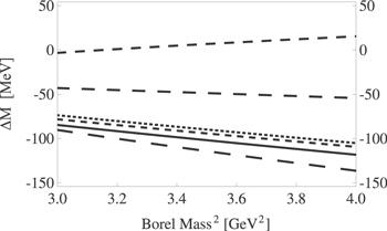
Figure 8. Mass corrections ${\rm{\Delta }}{M}^{{\bar{D}}^{(* )}{{\rm{\Sigma }}}_{c}^{(* )}}$ as functions of the Borel mass MB. The curves from top to bottom correspond to ${\rm{\Delta }}{M}_{I=1/2,J=1/2}^{{\bar{D}}^{* }{{\rm{\Sigma }}}_{c}^{* }}$, ${\rm{\Delta }}{M}_{I=1/2,J=3/2}^{{\bar{D}}^{* }{{\rm{\Sigma }}}_{c}^{* }}$, ${\rm{\Delta }}{M}_{I=1/2,J=3/2}^{{\bar{D}}^{* }{{\rm{\Sigma }}}_{c}}$, ${\rm{\Delta }}{M}_{I=1/2,J=3/2}^{\bar{D}{{\rm{\Sigma }}}_{c}^{* }}$, ${\rm{\Delta }}{M}_{I=1/2,J=1/2}^{\bar{D}{{\rm{\Sigma }}}_{c}}$, and ${\rm{\Delta }}{M}_{I=1/2,J=5/2}^{{\bar{D}}^{* }{{\rm{\Sigma }}}_{c}^{* }}$, respectively.

4.2. ${\bar{D}}^{(* )}{{\rm{\Lambda }}}_{c}$ molecules

In this subsection we investigate the light-quark-exchange term ΠQ(x) and study its contributions to the ${\bar{D}}^{(* )}{{\rm{\Lambda }}}_{c}$ molecules.
The currents corresponding to the $\bar{D}{{\rm{\Lambda }}}_{c}$ and ${\bar{D}}^{* }{{\rm{\Lambda }}}_{c}$ molecules are
$\begin{eqnarray}\begin{array}{l}{J}^{\bar{D}{{\rm{\Lambda }}}_{c}}(x)={J}^{\bar{D}}(x)\times {J}^{{{\rm{\Lambda }}}_{c}}(x)\\ \quad =[{\bar{c}}_{d}(x){\gamma }_{5}{q}_{d}(x)]\times [{\epsilon }^{{abc}}{q}_{a}^{{\rm{T}}}(x){\mathbb{C}}{\gamma }_{5}{q}_{b}(x){c}_{c}(x)],\end{array}\end{eqnarray}$
$\begin{eqnarray}\begin{array}{l}{J}_{\alpha }^{{\bar{D}}^{* }{{\rm{\Lambda }}}_{c}}(x)={J}_{\alpha }^{{\bar{D}}^{* }}(x)\times {J}^{{{\rm{\Lambda }}}_{c}}(x)\\ \quad =[{\bar{c}}_{d}(x){\gamma }_{\alpha }{q}_{d}(x)]\times [{\epsilon }^{{abc}}{q}_{a}^{{\rm{T}}}(x){\mathbb{C}}{\gamma }_{5}{q}_{b}(x){c}_{c}(x)].\end{array}\end{eqnarray}$
We use them to perform QCD sum rule analyses, and calculate mass corrections to the $\bar{D}{{\rm{\Lambda }}}_{c}$ molecule of J = 1/2 and the ${\bar{D}}^{* }{{\rm{\Lambda }}}_{c}$ molecule of J = 3/2. We find both of them to be positive. However, we do not obtain the mass correction to the ${\bar{D}}^{* }{{\rm{\Lambda }}}_{c}$ molecule of J = 1/2, just like the ${\bar{D}}^{* }{{\rm{\Sigma }}}_{c}$ molecule of J = 1/2 . These results suggest ${V}_{I=1/2,J=1/2}^{\bar{D}{{\rm{\Lambda }}}_{c}}(r)$ and ${V}_{I=1/2,J=3/2}^{{\bar{D}}^{* }{{\rm{\Lambda }}}_{c}}(r)$ to be both repulsive, so the J = 1/2 $\bar{D}{{\rm{\Lambda }}}_{c}$ and J = 3/2 ${\bar{D}}^{* }{{\rm{\Lambda }}}_{c}$ covalent molecules do not exist.

4.3. ${D}^{(* )}{\bar{K}}^{* }$ molecules

In this subsection we investigate the light-quark-exchange term ΠQ(x) and study its contributions to the ${D}^{(* )}{\bar{K}}^{* }$ molecules. We do not investigate the ${D}^{(* )}\bar{K}$ molecules in the present study, because their bare masses ${M}_{{D}^{(* )}}+{M}_{\bar{K}}$ can not be easily reached within the present QCD sum rule approach, due to the nature of K mesons as Nambu–Goldstone bosons.
The current corresponding to the $D{\bar{K}}^{* }$ molecule is
$\begin{eqnarray}\begin{array}{rcl}{J}_{\alpha }^{D{\bar{K}}^{* }}(x) & = & {J}^{\bar{D}}(x)\times {J}_{\alpha }^{{\bar{K}}^{* }}(x)\\ & = & [{\bar{q}}_{a}(x){\gamma }_{5}{c}_{a}(x)]\times [{\bar{q}}_{b}(x){\gamma }_{\alpha }{s}_{b}(x)].\end{array}\end{eqnarray}$
Its correlation function is
$\begin{eqnarray}\begin{array}{l}{{\rm{\Pi }}}_{\alpha \beta }^{D{\bar{K}}^{* }}({q}^{2})\\ \quad ={\rm{i}}\displaystyle \int {{\rm{d}}}^{4}x{{\rm{e}}}^{{\rm{i}}{qx}}\langle 0| {\mathbb{T}}\left[{J}_{\alpha }^{D{\bar{K}}^{* }}(x){J}_{\beta }^{D{\bar{K}}^{* },\dagger }(0)\right]| 0\rangle \\ \quad =\left({g}_{\alpha \beta }-\displaystyle \frac{{q}_{\alpha }{q}_{\beta }}{{q}^{2}}\right)\,{{\rm{\Pi }}}^{D{\bar{K}}^{* }}\left({q}^{2}\right)+\cdots .\end{array}\end{eqnarray}$
We use ${J}_{\alpha }^{D{\bar{K}}^{* }}(x)$ to perform QCD sum rule analyses, and calculate its mass correction to be
$\begin{eqnarray}{\rm{\Delta }}{M}_{I=0,J=1}^{D{\bar{K}}^{* }}=-180\,\mathrm{MeV}.\end{eqnarray}$
This suggests ${V}_{I=0,J=1}^{D{\bar{K}}^{* }}(r)$ to be attractive, so there can be the $D{\bar{K}}^{* }$ covalent molecule of I = 0 and J = 1.
The current corresponding to the ${D}^{* }{\bar{K}}^{* }$ molecule is
$\begin{eqnarray}\begin{array}{rcl}{J}_{{\alpha }_{1}{\alpha }_{2}}^{{D}^{* }{\bar{K}}^{* }}(x) & = & {J}_{{\alpha }_{1}}^{{\bar{D}}^{* }}(x)\times {J}_{{\alpha }_{2}}^{{\bar{K}}^{* }}(x)\\ & = & [{\bar{q}}_{a}(x){\gamma }_{{\alpha }_{1}}{c}_{a}(x)]\times [{\bar{q}}_{b}(x){\gamma }_{{\alpha }_{2}}{s}_{b}(x)].\end{array}\end{eqnarray}$
Its correlation function is
$\begin{eqnarray}\begin{array}{l}{{\rm{\Pi }}}_{{\alpha }_{1}{\alpha }_{2},{\beta }_{1}{\beta }_{2}}^{{D}^{* }{\bar{K}}^{* }}({q}^{2})\\ \quad ={\rm{i}}\displaystyle \int {{\rm{d}}}^{4}x{{\rm{e}}}^{{\rm{i}}{qx}}\langle 0| {\mathbb{T}}\left[{J}_{{\alpha }_{1}{\alpha }_{2}}^{{D}^{* }{\bar{K}}^{* }}(x){J}_{{\beta }_{1}{\beta }_{2}}^{{D}^{* }{\bar{K}}^{* },\dagger }(0)\right]| 0\rangle \\ \quad ={{ \mathcal G }}_{{\alpha }_{1}{\alpha }_{2},{\beta }_{1}{\beta }_{2}}^{2}({q}^{2})\,{{\rm{\Pi }}}_{J=2}^{{D}^{* }{\bar{K}}^{* }}\left({q}^{2}\right)\\ \quad +{{ \mathcal G }}_{{\alpha }_{1}{\alpha }_{2},{\beta }_{1}{\beta }_{2}}^{1}({q}^{2})\,{{\rm{\Pi }}}_{J=1}^{{D}^{* }{\bar{K}}^{* }}\left({q}^{2}\right)\\ \quad +{{ \mathcal G }}_{{\alpha }_{1}{\alpha }_{2},{\beta }_{1}{\beta }_{2}}^{0}({q}^{2})\,{{\rm{\Pi }}}_{J=0}^{{D}^{* }{\bar{K}}^{* }}\left({q}^{2}\right)+\cdots ,\end{array}\end{eqnarray}$
where ${{\rm{\Pi }}}_{J=2}^{{D}^{* }{\bar{K}}^{* }}\left({q}^{2}\right)$, ${{\rm{\Pi }}}_{J=1}^{{D}^{* }{\bar{K}}^{* }}\left({q}^{2}\right)$, and ${{\rm{\Pi }}}_{J=0}^{{D}^{* }{\bar{K}}^{* }}\left({q}^{2}\right)$ are contributed by the spin-2, spin-1, and spin-0 components, respectively. ${{ \mathcal G }}_{{\alpha }_{1}{\alpha }_{2},{\beta }_{1}{\beta }_{2}}^{2}({q}^{2})$, ${{ \mathcal G }}_{{\alpha }_{1}{\alpha }_{2},{\beta }_{1}{\beta }_{2}}^{1}({q}^{2})$, and ${{ \mathcal G }}_{{\alpha }_{1}{\alpha }_{2},{\beta }_{1}{\beta }_{2}}^{0}({q}^{2})$ are coefficients of the spin-2, spin-1, and spin-0 propagators, respectively:
$\begin{eqnarray}\begin{array}{l}{{ \mathcal G }}_{{\alpha }_{1}{\alpha }_{2},{\beta }_{1}{\beta }_{2}}^{2}({q}^{2})=\displaystyle \frac{{g}_{{\alpha }_{1}{\beta }_{1}}{g}_{{\alpha }_{2}{\beta }_{2}}}{2}\\ \quad +\displaystyle \frac{{g}_{{\alpha }_{1}{\beta }_{2}}{g}_{{\alpha }_{2}{\beta }_{1}}}{2}-\displaystyle \frac{{g}_{{\alpha }_{1}{\alpha }_{2}}{g}_{{\beta }_{1}{\beta }_{2}}}{4},\end{array}\end{eqnarray}$
$\begin{eqnarray}{{ \mathcal G }}_{{\alpha }_{1}{\alpha }_{2},{\beta }_{1}{\beta }_{2}}^{1}({q}^{2})=\displaystyle \frac{{g}_{{\alpha }_{1}{\beta }_{1}}{g}_{{\alpha }_{2}{\beta }_{2}}}{2}-\displaystyle \frac{{g}_{{\alpha }_{1}{\beta }_{2}}{g}_{{\alpha }_{2}{\beta }_{1}}}{2},\end{eqnarray}$
$\begin{eqnarray}{{ \mathcal G }}_{{\alpha }_{1}{\alpha }_{2},{\beta }_{1}{\beta }_{2}}^{0}({q}^{2})={g}_{{\alpha }_{1}{\alpha }_{2}}{g}_{{\beta }_{1}{\beta }_{2}}.\end{eqnarray}$
We use ${J}_{{\alpha }_{1}{\alpha }_{2}}^{{D}^{* }{\bar{K}}^{* }}(x)$ to perform QCD sum rule analyses, and extract mass corrections to the three isoscalar ${D}^{* }{\bar{K}}^{* }$ molecules of J = 2, J = 1, and J = 0:
$\begin{eqnarray}{\rm{\Delta }}{M}_{I=0,J=2}^{{D}^{* }{\bar{K}}^{* }}=-119\,\mathrm{MeV},\end{eqnarray}$
$\begin{eqnarray}{\rm{\Delta }}{M}_{I=0,J=1}^{{D}^{* }{\bar{K}}^{* }}=-46\,\mathrm{MeV},\end{eqnarray}$
$\begin{eqnarray}{\rm{\Delta }}{M}_{I=0,J=0}^{{D}^{* }{\bar{K}}^{* }}=-4.5\,\mathrm{MeV}.\end{eqnarray}$
These results suggest ${V}_{I=0,J=2}^{{D}^{* }{\bar{K}}^{* }}(r)$ to be attractive, so there can be the ${D}^{* }{\bar{K}}^{* }$ covalent molecule of I = 0 and J = 2.
We show variations of ${\rm{\Delta }}{M}^{{D}^{(* )}{\bar{K}}^{* }}$ in figure 9 with respect to the Borel mass MB. Especially, ${V}_{I=0,J=0}^{{D}^{* }{\bar{K}}^{* }}(r)$ depends significantly on the Borel mass MB and so also on the threshold value s0, for which we refer to section 5 for relevant model-independent discussions.
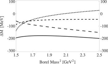
Figure 9. Mass corrections ${\rm{\Delta }}{M}^{{D}^{(* )}{\bar{K}}^{* }}$ as functions of the Borel mass MB. The curves from top to bottom correspond to ${\rm{\Delta }}{M}_{I=0,J=0}^{{D}^{* }{\bar{K}}^{* }}$ (short-dashed), ${\rm{\Delta }}{M}_{I=0,J=1}^{{D}^{* }{\bar{K}}^{* }}$ (middle-dashed), ${\rm{\Delta }}{M}_{I=0,J=2}^{{D}^{* }{\bar{K}}^{* }}$ (long-dashed), and ${\rm{\Delta }}{M}_{I=0,J=1}^{D{\bar{K}}^{* }}$ (solid), respectively.
For completeness, we study the isovector ${D}^{(* )}{\bar{K}}^{* }$ molecules and obtained
$\begin{eqnarray}{\rm{\Delta }}{M}_{I=1}^{D{\bar{K}}^{* }/{D}^{* }{\bar{K}}^{* }}\approx -{\rm{\Delta }}{M}_{I=0}^{D{\bar{K}}^{* }/{D}^{* }{\bar{K}}^{* }}.\end{eqnarray}$

4.4. ${D}^{(* )}{\bar{D}}^{(* )}$ molecules

The light-quark-exchange term ΠQ(x) does not contribute to the correlation functions of the ${D}^{(* )}{\bar{D}}^{(* )}$ molecules, suggesting the ${D}^{(* )}{\bar{D}}^{(* )}$ covalent molecules not to exist. However, there can still be the ${D}^{(* )}{\bar{D}}^{(* )}$ hadronic molecular states induced by some other binding mechanisms, such as the one-meson-exchange interaction [2332].

5. Covalent hadronic molecule

In the previous section we applied QCD sum rules to study the binding mechanism induced by shared light quarks. This mechanism is somewhat similar to the covalent bond in chemical molecules induced by shared electrons, so we call such hadronic molecules ‘covalent hadronic molecules'. Recalling that the two shared electrons must spin in opposite directions (and so totally antisymmetric obeying the Pauli principle) in order to form a chemical covalent bond, our QCD sum rule results indicate a similar behavior: the light-quark-exchange interaction is attractive when the shared light quarks are totally antisymmetric so that obey the Pauli principle (these quarks may spin in the same direction given their flavor structure capable of being antisymmetric).
In this section we qualitatively study the above hypothesis. Its logical chain is quite straightforward. We assume the two light quarks qA inside Y and qB inside Z are totally antisymmetric. Hence, qA and qB obey the Pauli principle, so that they can be exchanged and shared. By doing this, wave functions of Y and Z overlap with each other, so that they are attracted and there can be the covalent hadronic molecule X = ∣YZ⟩. This picture has been depicted in figure 2. We believe it is better and more important than our QCD sum rule results, given it is model-independent and more easily applicable.
We apply it to study several examples as follows. The two exchanged light quarks have the same color and so the symmetric color structure; besides, we assume their orbital structure to be S-wave and so also symmetric; consequently, we only need to investigate their spin and flavor structures.
a. ${\bar{D}}^{(* )0}[{\bar{c}}_{1}{u}_{2}]$–${{\rm{\Lambda }}}_{c}^{+}[{u}_{3}{d}_{4}{c}_{5}]$ covalent molecules. Let us exchange u2 inside ${\bar{D}}^{(* )0}$ and u3 inside ${{\rm{\Lambda }}}_{c}^{+}$. u3 and d4 inside ${{\rm{\Lambda }}}_{c}^{+}$ spin in opposite directions, u2 and d4 also need to spin in opposite directions in order to form another ${{\rm{\Lambda }}}_{c}^{+}$, so u2 and u3 spin in the same direction with the symmetric spin structure. The flavor structure of u2 and u3 is also symmetric, so they are totally symmetric (S = symmetric and A = antisymmetric):
color flavor spin orbital total
u2u3 S S S S S
Accordingly, the ${\bar{D}}^{(* )}{{\rm{\Lambda }}}_{c}$ covalent molecules do not exist. This is consistent with our QCD sum rule result obtained in section 4.2.
b. ${\bar{D}}^{0}[{\bar{c}}_{1}{u}_{2}]$–${{\rm{\Sigma }}}_{c}^{+}[{u}_{3}{d}_{4}{c}_{5}]$ covalent molecule. Let us exchange u2 inside ${\bar{D}}^{0}$ and u3 inside ${{\rm{\Sigma }}}_{c}^{+}$. ${\bar{c}}_{1}$ and u2 inside ${\bar{D}}^{0}$ spin in opposite directions, ${\bar{c}}_{1}$ and u3 also need to spin in opposite directions in order to form another ${\bar{D}}^{0}$, so u2 and u3 spin in the same direction with the symmetric spin structure. The flavor structure of u2 and u3 is also symmetric, so they are totally symmetric:
color flavor spin orbital total
u2u3 S S S S S
Accordingly, the ${\bar{D}}^{0}{{\rm{\Sigma }}}_{c}^{+}$ covalent molecule does not exist, consistent with section 3.3.
c. $\bar{D}[{\bar{c}}_{1}{q}_{2}]$–Σc[q3q4c5] covalent molecule (q = u/d). After including the isospin symmetry, the exchange can take place between up and down quarks. Let us exchange q2 inside $\bar{D}$ and q3 inside Σc. As discussed above, they have the symmetric spin structure, so they can be totally antisymmetric as long as their flavor structure is antisymmetric:
color flavor spin orbital total
q2q3 S A S S A
Accordingly, there can be the I = 1/2 $\bar{D}{{\rm{\Sigma }}}_{c}$ covalent molecule, but not the I = 3/2 one. This is consistent with our QCD sum rule result obtained in sections 3.1 and 3.4. Similarly, we derive that there can be the I = 1/2 $\bar{D}{{\rm{\Sigma }}}_{c}^{* }$ and I = 0 $D{\bar{K}}^{* }$ covalent molecules, consistent with sections 4.1 and 4.3.
d. J = 5/2 ${\bar{D}}^{* }[{\bar{c}}_{1}{q}_{2}]$–${{\rm{\Sigma }}}_{c}^{* }[{q}_{3}{q}_{4}{c}_{5}]$ covalent molecule. Let us exchange q2 inside ${\bar{D}}^{* }$ and q3 inside ${{\rm{\Sigma }}}_{c}^{* }$. In the Jz = +5/2 component, all the quarks/antiquark spin in the same direction, so q2 and q3 have the symmetric spin structure. They can be totally antisymmetric as long as their flavor structure is antisymmetric:
color flavor spin orbital total
q2q3 S A S S A
Accordingly, there can be the I = 1/2 ${\bar{D}}^{* }{{\rm{\Sigma }}}_{c}^{* }$ covalent molecule of J = 5/2, but not the I = 3/2 one. This is consistent with our QCD sum rule result obtained in section 4.1. Similarly, we derive that there can be the ${D}^{* }{\bar{K}}^{* }$ covalent molecule of I = 0 and J = 2, consistent with section 4.3.
e. J = 0 ${D}^{* }[{c}_{1}{\bar{q}}_{2}]$–${\bar{K}}^{* }[{s}_{3}{\bar{q}}_{4}]$ covalent molecule. Let us exchange ${\bar{q}}_{2}$ inside D* and ${\bar{q}}_{4}$ inside ${\bar{K}}^{* }$. We perform the spin decomposition (see appendix B):
$\begin{eqnarray}\begin{array}{l}\left|{1}_{c\bar{q}}\otimes {1}_{s\bar{q}};J=\,0\right\rangle \\ \quad =\,\displaystyle \frac{\sqrt{3}}{2}\,\left|{0}_{{cs}}\otimes {0}_{\bar{q}\bar{q}};J=0\right\rangle -\displaystyle \frac{1}{2}\,\left|{1}_{{cs}}\otimes {1}_{\bar{q}\bar{q}};J=0\right\rangle .\end{array}\end{eqnarray}$
Hence, there exists both ${s}_{{\bar{q}}_{2}{\bar{q}}_{4}}=0$ (75%) and ${s}_{{\bar{q}}_{2}{\bar{q}}_{4}}=1$ (25%) components. The former becomes attractive when I = 1, and the latter becomes attractive when I = 0:
color flavor spin orbital total
${\bar{q}}_{2}\leftrightarrow {\bar{q}}_{4}$ S S A S A
${\bar{q}}_{2}\leftrightarrow {\bar{q}}_{4}$ S A S S A
It is well known that there are both the para-hydrogen and ortho-hydrogen, where the two protons spin in opposite directions and in the same direction, respectively. Similarly, there might be two J = 0 ${D}^{* }{\bar{K}}^{* }$ covalent molecules, i.e. the two components $\left|{0}_{{cs}}\otimes {0}_{\bar{q}\bar{q}};J=0\right\rangle $ of I = 1 and $\left|{1}_{{cs}}\otimes {1}_{\bar{q}\bar{q}};J=0\right\rangle $ of I = 0. However, our QCD sum rule studies performed in section 4.3 can not differentiate these two hyperfine structures, because there we have summed over the D* and ${\bar{K}}^{* }$ polarizations.
It is useful to generally discuss how many light quarks at most are there in the lowest orbit (q = u/d):
1.

1.In the ${\bar{D}}^{(* )}[{\bar{c}}_{1}{q}_{2}]{K}^{(* )}[{\bar{s}}_{3}{q}_{4}]$ covalent molecule, the two exchanged light quarks q2 and q4 have the same color and so the symmetric color structure; besides, we assume their orbital structure to be S-wave and so also symmetric; consequently, there are two possible configurations satisfying the Pauli principle (S = symmetric and A = antisymmetric):

color flavor spin orbital total
q2q4 S A S S A
q2q4 S S A S A
Hence, two antiquarks can share (at most) two quarks, with the quantum numbers either (I)JP = (0)1+ or (1)0+.

2.

2.In the ${\bar{D}}^{(* )}[{\bar{c}}_{1}{q}_{2}]$–${{\rm{\Sigma }}}_{c}^{(* )}[{q}_{3}{q}_{4}{c}_{5}]$ covalent molecule, there is three light up/down quarks. We assume the two exchanged quarks to be q2 and q3 with the same color. There are also two possible configurations:

color flavor spin orbital total
q2q3 S A S S A
q2q4 A S S S A
q3q4 A S S S A

q2q3 S S A S A
q2q4 A S S S A
q3q4 A S S S A
They satisfy the condition that any two of the three light quarks are totally antisymmetric so they obey the Pauli principle. Hence, one quark and one antiquark can share (at most) three quarks, with either $(I){J}^{P}=\left(\displaystyle \frac{1}{2}\right){\displaystyle \frac{3}{2}}^{+}$ or $\left(\displaystyle \frac{3}{2}\right){\displaystyle \frac{1}{2}}^{+}$. However, the ${\bar{D}}^{(* )}{{\rm{\Lambda }}}_{c}$ system does not satisfy this condition.

3.

3.In the ${{\rm{\Sigma }}}_{c}^{(* )}[{q}_{1}{q}_{2}{c}_{3}]$–${{\rm{\Sigma }}}_{b}^{(* )}[{q}_{4}{q}_{5}{c}_{6}]$ covalent molecule, there is four light up/down quarks. We assume that q1 and q4 can be exchanged with the same color, and q2 and q5 can also be exchanged with the same color. There can be four possible configurations:

color flavor spin orbital total
q1q4 S A S S A
q2q5 S A S S A
q1q2 A S S S A
q1q5 A S S S A
q2q4 A S S S A
q4q5 A S S S A

q1q4 S S A S A
q2q5 S A S S A

q1q4 S A S S A
q2q5 S S A S A

q1q4 S S A S A
q2q5 S S A S A
They satisfy that any two of the four light quarks are totally antisymmetric so they obey the Pauli principle. Hence, two quarks can share (at most) four quarks, with (I)JP = (0)2+/(1)1+/(2)0+. However, neither ${{\rm{\Sigma }}}_{c}^{(* )}{{\rm{\Lambda }}}_{b}$ nor ΛbΛb satisfies this condition.
We apply the above model-independent hypothesis to qualitatively predict more covalent hadronic molecules:

Induced by shared light up/down quarks, there can be the I = 0 ${\bar{D}}^{(* )}[\bar{c}q]$–${B}^{(* )}[\bar{b}q]$, I = 0 ${\bar{D}}^{(* )}[\bar{c}q]$–${{\rm{\Xi }}}_{c}^{(^{\prime} * )}[{csq}]$, I = 0 ${{\rm{\Sigma }}}_{c}^{(* )}[{cqq}]$–${{\rm{\Sigma }}}_{b}^{(* )}[{bqq}]$, and I = 1/2 ${{\rm{\Sigma }}}_{c}^{(* )}[{cqq}]$–${{\rm{\Xi }}}_{b}^{(^{\prime} * )}[{bsq}]$ covalent molecules, etc. We roughly estimate their binding energies to be at the 10 MeV level, considering the Pc/Pcs and X0(2900) [66, 67] as possible covalent hadronic molecules. We list them in table 1, which are still waiting to be carefully analysed.

If the strange quark is also exchangeable, there can be the ${\bar{D}}_{s}^{(* )}[\bar{c}s]$–${B}^{(* )}[\bar{b}q]$ and ${\bar{D}}_{s}^{(* )}[\bar{c}s]$–${{\rm{\Xi }}}_{c}^{(^{\prime} * )}[{csq}]$ covalent molecules, etc. These states are induced by shared light up/down/strange quarks, with the SU(3) light flavor structure being antisymmetric.

If the heavy-quark-exchange interaction is negligible, there might be the I = 0 ${\bar{D}}^{(* )}[\bar{c}q]$–${\bar{D}}^{(* )}[\bar{c}q]$, I = 0 ${{\rm{\Sigma }}}_{c}^{(* )}[{cqq}]$–${{\rm{\Sigma }}}_{c}^{(* )}[{cqq}]$, and I = 1/2 ${{\rm{\Sigma }}}_{c}^{(* )}[{cqq}]$–${{\rm{\Xi }}}_{c}^{(^{\prime} * )}[{csq}]$ covalent molecules, etc. These states are still induced by shared light up/down quarks.

Especially, we propose to search for the ${D}^{* -}[\bar{c}d]$–${K}^{* 0}[\bar{s}d]$, ${D}^{* -}[\bar{c}d]$–${D}^{* -}[\bar{c}d]$, and ${D}^{* -}[\bar{c}d]$–${B}^{* 0}[\bar{b}d]$ covalent molecules of I = 1 and J = 0. These states might exist, when the two light quarks spin in opposite directions and the two antiquarks also spin in opposite directions, just like the para-hydrogen.

Table 1. Possibly-existing covalent hadronic molecules $\left|(I){J}^{P}\right\rangle $ induced by shared light up/down quarks, derived from the hypothesis that the light-quark-exchange interaction is attractive when the shared light quarks are totally antisymmetric so that they obey the Pauli principle. Here, q and s denote the light up/down and strange quarks, respectively; Q and ${Q}^{{\prime} }$ denote two different heavy quarks; the symbols [AB] = ABBA and {AB} = AB + BA denote the antisymmetric and symmetric SU(3) light flavor structures, respectively. The states with ✓have been confirmed in QCD sum rule calculations of the present study, but the states with ? and ?? have not. This is because the latter contain relatively-polarized components, while one needs to sum over polarizations of these components within QCD sum rule method and so can not differentiate these hyperfine structures. Moreover, the states with ?? contain light up/down quarks with the symmetric flavor/isospin structure, whose masses are (probably) considerably larger than their partners with the antisymmetric flavor/isospin structure. The states without any identification are still waiting to be carefully analysed in our future QCD sum rule studies.
$\left|\bar{Q}q,\displaystyle \frac{1}{2}{0}^{-}\right\rangle $ $\left|\bar{Q}q,\displaystyle \frac{1}{2}{1}^{-}\right\rangle $ $\left|Q[{qq}],0{\displaystyle \frac{1}{2}}^{+}\right\rangle $ $\left|Q\{{qq}\},1{\displaystyle \frac{1}{2}}^{+}\right\rangle $ $\left|Q\{{qq}\},1{\displaystyle \frac{3}{2}}^{+}\right\rangle $ $\left|Q[{sq}],\displaystyle \frac{1}{2}{\displaystyle \frac{1}{2}}^{+}\right\rangle $ $\left|Q\{{sq}\},\displaystyle \frac{1}{2}{\displaystyle \frac{1}{2}}^{+}\right\rangle $ $\left|Q\{{sq}\},\displaystyle \frac{1}{2}{\displaystyle \frac{3}{2}}^{+}\right\rangle $
$\left|{\bar{Q}}^{{\prime} }q,\displaystyle \frac{1}{2}{0}^{-}\right\rangle $ $\left|(0){0}^{+}\right\rangle $ $\left|(0){1}^{+}\right\rangle $ (✓) $\left|(\displaystyle \frac{1}{2}){\displaystyle \frac{1}{2}}^{-}\right\rangle $ (✓) $\left|(\displaystyle \frac{1}{2}){\displaystyle \frac{3}{2}}^{-}\right\rangle $ (✓) $\left|(0){\displaystyle \frac{1}{2}}^{-}\right\rangle $ $\left|(0){\displaystyle \frac{1}{2}}^{-}\right\rangle $ $\left|(0){\displaystyle \frac{3}{2}}^{-}\right\rangle $
$\left|{\bar{Q}}^{{\prime} }q,\displaystyle \frac{1}{2}{1}^{-}\right\rangle $ $\begin{array}{c}\left|(0){0}^{+}\right\rangle \,(?)\\ \left|(1){0}^{+}\right\rangle \,(??)\\ \left|(0){1}^{+}\right\rangle \,(?)\\ \left|(1){1}^{+}\right\rangle \,(??)\\ \left|(0){2}^{+}\right\rangle \,(\checkmark )\end{array}$ $\begin{array}{c}\left|(\displaystyle \frac{1}{2}){\displaystyle \frac{1}{2}}^{-}\right\rangle \,(?)\\ \left|(\displaystyle \frac{3}{2}){\displaystyle \frac{1}{2}}^{-}\right\rangle \,(??)\\ \left|(\displaystyle \frac{1}{2}){\displaystyle \frac{3}{2}}^{-}\right\rangle \,(\checkmark )\\ \left|(\displaystyle \frac{3}{2}){\displaystyle \frac{3}{2}}^{-}\right\rangle \,(??)\end{array}$ $\begin{array}{c}\left|(\displaystyle \frac{1}{2}){\displaystyle \frac{1}{2}}^{-}\right\rangle \,(?)\\ \left|(\displaystyle \frac{3}{2}){\displaystyle \frac{1}{2}}^{-}\right\rangle \,(??)\\ \left|(\displaystyle \frac{1}{2}){\displaystyle \frac{3}{2}}^{-}\right\rangle \,(?)\\ \left|(\displaystyle \frac{3}{2}){\displaystyle \frac{3}{2}}^{-}\right\rangle \,(??)\\ \left|(\displaystyle \frac{1}{2}){\displaystyle \frac{5}{2}}^{-}\right\rangle \,(\checkmark )\end{array}$ $\begin{array}{c}\left|(0){\displaystyle \frac{1}{2}}^{-}\right\rangle \\ \left|(0){\displaystyle \frac{3}{2}}^{-}\right\rangle \end{array}$ $\begin{array}{c}\left|(0){\displaystyle \frac{1}{2}}^{-}\right\rangle \\ \left|(1){\displaystyle \frac{1}{2}}^{-}\right\rangle \\ \left|(0){\displaystyle \frac{3}{2}}^{-}\right\rangle \\ \left|(1){\displaystyle \frac{3}{2}}^{-}\right\rangle \end{array}$ $\begin{array}{c}\left|(0){\displaystyle \frac{1}{2}}^{-}\right\rangle \\ \left|(1){\displaystyle \frac{1}{2}}^{-}\right\rangle \\ \left|(0){\displaystyle \frac{3}{2}}^{-}\right\rangle \\ \left|(1){\displaystyle \frac{3}{2}}^{-}\right\rangle \\ \left|(0){\displaystyle \frac{5}{2}}^{-}\right\rangle \end{array}$

$\left|Q[{qq}],0{\displaystyle \frac{1}{2}}^{+}\right\rangle $

$\left|Q\{{qq}\},1{\displaystyle \frac{1}{2}}^{+}\right\rangle $ $\begin{array}{c}\left|(0){1}^{+}\right\rangle \\ \left|(1)0/{1}^{+}\right\rangle \\ \left|(2)0/{1}^{+}\right\rangle \end{array}$ $\begin{array}{c}\left|(0)1/{2}^{+}\right\rangle \\ \left|(1)1/{2}^{+}\right\rangle \\ \left|(2){1}^{+}\right\rangle \end{array}$ $\left|(\displaystyle \frac{1}{2})0/{1}^{+}\right\rangle $ $\begin{array}{c}\left|(\displaystyle \frac{1}{2})0/{1}^{+}\right\rangle \\ \left|(\displaystyle \frac{3}{2})0/{1}^{+}\right\rangle \end{array}$ $\begin{array}{c}\left|(\displaystyle \frac{1}{2})1/{2}^{+}\right\rangle \\ \left|(\displaystyle \frac{3}{2})1/{2}^{+}\right\rangle \end{array}$

$\left|Q\{{qq}\},1{\displaystyle \frac{3}{2}}^{+}\right\rangle $ $\begin{array}{c}\left|(0)1/2/{3}^{+}\right\rangle \\ \left|(1)0/1/{2}^{+}\right\rangle \\ \left|(2)0/{1}^{+}\right\rangle \end{array}$ $\left|(\displaystyle \frac{1}{2})1/{2}^{+}\right\rangle $ $\begin{array}{c}\left|(\displaystyle \frac{1}{2})1/{2}^{+}\right\rangle \\ \left|(\displaystyle \frac{3}{2})1/{2}^{+}\right\rangle \end{array}$ $\begin{array}{c}\left|(\displaystyle \frac{1}{2})0/1/2/{3}^{+}\right\rangle \\ \left|(\displaystyle \frac{3}{2})0/1/{2}^{+}\right\rangle \end{array}$

6. A toy model to formulize covalent hadronic molecules

In the previous section we have qualitatively discussed the hypothesis: the light-quark-exchange interaction is attractive when the shared light quarks are totally antisymmetric so that they obey the Pauli principle. In this section we further build a toy model to quantitatively formulize it, and estimate binding energies of some possibly-existing covalent hadronic molecules.
We shall use the following formula to estimate binding energies of the ${\bar{D}}^{(* )}{{\rm{\Sigma }}}_{c}^{(* )}$, ${D}^{(* )}{\bar{B}}^{(* )}$, and ${{\rm{\Sigma }}}_{c}^{(* )}{{\rm{\Sigma }}}_{b}^{(* )}$ hadronic molecules:
$\begin{eqnarray}B={N}_{A}A-{N}_{R}R-N\epsilon -\kappa \langle {\lambda }_{c}\cdot {\lambda }_{\bar{c}/b}\,{s}_{c}\cdot {s}_{\bar{c}/b}\rangle .\end{eqnarray}$
This formula will be explained in section 6.1 in details, and similar formulae are used for some other covalent hadronic molecules. There are altogether four parameters:
$\begin{eqnarray}A\sim 30\,\mathrm{MeV},\end{eqnarray}$
$\begin{eqnarray}R\sim 17\,\mathrm{MeV},\end{eqnarray}$
$\begin{eqnarray}\epsilon \sim 6\,\mathrm{MeV},\end{eqnarray}$
$\begin{eqnarray}\kappa \sim 13\,\mathrm{MeV},\end{eqnarray}$
which are estimated by considering the Pc/Pcs and the recently observed ${T}_{{cc}}^{+}$ as possible covalent hadronic molecules.

6.1. Parameters

As discussed in the previous section, there exists an attractive interaction when exchanging up and down quarks with the configuration:
color flavor spin orbital total
$q\leftrightarrow {q}^{{\prime} }$ S A S S A
These two light up/down quarks have the same color and their relative orbital structure is S-wave. Besides, they have the antisymmetric flavor structure and the symmetric spin structure, so with the quantum numbers (I)JP = (0)1+. We use the attractive bond energy A to describe this attraction, which is estimated to be A ∼ 30 MeV for each bond, with NA the number of such bonds. It is illustrated in figure 10 using the solid curve.
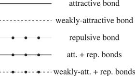
Figure 10. (Weakly-)Attractive and repulsive covalent hadronic bonds as well as their combinations. In the present study we take into account the attractive bond and its combination with the repulsive bond, whose bond energies are estimated to be A ∼ 30 MeV and AR ∼ 13 MeV, respectively.
As discussed in the previous section, the two exchanged light up/down quarks can form another configuration of (I)JP = (1)0+:
color flavor spin orbital total
$q\leftrightarrow {q}^{{\prime} }$ S S A S A
However, its induced interaction is weaker, so we do not take this configuration into account in the present study. It is illustrated in figure 10 using the dashed curve.
There exists an (I)JP = (0)0+ up–down quark pair inside the proton/neutron with the configuration:
color flavor spin orbital total
q1q2 A A A S A
One can not exchange q1 (nor q2) with another light up/down quark q3, at the same time keeping: (a) any two of the three light quarks are totally antisymmetric, and (b) the proton/neutron remains unchanged. As an example, we exchange q1q3 and keep (b), but then (a) is not satisfied:
color flavor spin orbital total
q1q2 A A A S A
q2q3 A A A S A
q1q3 S S S S S
Therefore, the above up–down quark pair is in some sense ‘saturated'. This suggests that the (I)JP = (0)0+ up–down quark pairs inside protons/neutrons can not be exchanged, so they are capable of forming repulsive cores in the nucleus.
We use the repulsive bond energy R to describe the repulsion between two repulsive cores, which is estimated to be R ∼ 17 MeV for each bond, with NR the number of such bonds. It is illustrated in figure 10 using the dotted curve. Besides, we shall find in sections 6.3 and 6.4 that the two charm quarks can also form such repulsive cores in D(*)D(*) and ${{\rm{\Sigma }}}_{c}^{(* )}{{\rm{\Sigma }}}_{c}^{(* )}$ hadronic molecules, etc.
The third parameter is the residual energy ε, which is estimated to be ε ∼ 6 MeV for each component hadron, with N the number of components. We use it to describe the part of kinetic energy that can not be absorbed into A and R.
The fourth parameter κ relates to the spin splitting. We use the following term to describe the interaction between the c and $\bar{c}$ quarks when investigating ${\bar{D}}^{(* )}{{\rm{\Sigma }}}_{c}^{(* )}$ hadronic molecules:
$\begin{eqnarray}{{ \mathcal H }}_{{\rm{spin}}}=-\kappa \,\langle {\lambda }_{c}\cdot {\lambda }_{\bar{c}}\,{s}_{c}\cdot {s}_{\bar{c}}\rangle ,\end{eqnarray}$
where κ is estimated to be κ ∼ 13 MeV; sc and ${s}_{\bar{c}}$ are spins of the c and $\bar{c}$ quarks; λc and ${\lambda }_{\bar{c}}$ are their color charges. We use a similar term to describe the interaction between the c and b quarks when investigating ${D}^{(* )}{\bar{B}}^{(* )}$ and ${{\rm{\Sigma }}}_{c}^{(* )}{{\rm{\Sigma }}}_{b}^{(* )}$ hadronic molecules:
$\begin{eqnarray}{{ \mathcal H }}_{{\rm{spin}}}^{{\prime} }=-\kappa \,\langle {\lambda }_{c}\cdot {\lambda }_{b}\,{s}_{c}\cdot {s}_{b}\rangle .\end{eqnarray}$
However, we do not include such terms when investigating D(*)D(*) and ${{\rm{\Sigma }}}_{c}^{(* )}{{\rm{\Sigma }}}_{c}^{(* )}$ hadronic molecules, since the interaction between two charm quarks has been (partly) taken into account in the repulsive bond energy R. Note that the spin splitting effect in hadronic molecules still needs to be updated with future experiments, since we do not well understand it at this moment. See section 6.7 for more discussions.

6.2. Nucleus

Taking the proton/neutron as the combination of an (I)JP = (0)0+ up–down quark pair together with another up/down quark, we can estimate binding energies of the 2H, 3H, 3He, and 4He, as illustrated in figure 11. In the present study we do not investigate other nuclei consisting of more nucleons, because there are at most two up and two down quarks in the lowest orbit. See section 6.6 for relevant studies on the hypernucleus.
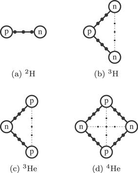
Figure 11. Illustration of the 2H, 3H, 3He, and 4He in our model. The shape of 4He is a tetrahedron other than a square.
The 2H contains two shared light up/down quarks with the configuration of (I)JP = (0)1+:
color flavor spin orbital total
q1q2 S A S S A
We estimate its binding energy to be
$\begin{eqnarray}{B}_{I=0,J=1}^{{}^{2}{\rm{H}}}=A-R-2\epsilon \sim 1\,\mathrm{MeV}.\end{eqnarray}$
The 3H and 3He both contain three shared light up/down quarks with the configuration of (I)JP = (1/2)1/2+:
color flavor spin orbital total
q1q2 S A S S A
q1q3 S A S S A
q2q3 S S A S A
We estimate their binding energies to be
$\begin{eqnarray}{B}_{I=1/2,J=1/2}^{{}^{3}{\rm{H}}{/}^{3}\mathrm{He}}=2A-2R-3\epsilon \sim 8\,\mathrm{MeV}.\end{eqnarray}$
The 4He contains four shared light up/down quarks with the configuration of (I)JP = (0)0+:
color flavor spin orbital total
q1q2 S S A S A
q1q3 S A S S A
q1q4 S A S S A
q2q3 S A S S A
q2q4 S A S S A
q3q4 S S A S A
We estimate its binding energy to be
$\begin{eqnarray}{B}_{I=0,J=0}^{{}^{4}\mathrm{He}}=4A-4R-4\epsilon \sim 28\,\mathrm{MeV}.\end{eqnarray}$

6.3. ${D}^{(* )}{D}^{(* )}/{D}^{(* )}{\bar{B}}^{(* )}/{\bar{B}}^{(* )}{\bar{B}}^{(* )}$ molecules

The (I)JP = (0)0+ DD hadronic molecule does not exist due to the Bose–Einstein statistics. So do the D*D* molecules of (I)JP = (0)0+ and (I)JP = (0)2+. Actually, we can construct their corresponding currents, and explicitly prove them to be zero.
Similar to section 2, we investigate the (I)JP = (0)1+ DD* hadronic molecule through its corresponding current:
$\begin{eqnarray}\begin{array}{rcl}\sqrt{2}{J}_{\alpha }^{{{DD}}^{* }} & = & {J}_{\alpha }^{{D}^{+}{D}^{* 0}}-{J}_{\alpha }^{{D}^{0}{D}^{* +}}\\ & = & {J}^{{D}^{+}}\times {J}_{\alpha }^{{D}^{* 0}}-{J}^{{D}^{0}}\times {J}_{\alpha }^{{D}^{* +}}\\ & = & {\bar{d}}_{a}{\gamma }_{5}{c}_{a}\,{\bar{u}}_{b}{\gamma }_{\alpha }{c}_{b}-{\bar{u}}_{a}{\gamma }_{5}{c}_{a}\,{\bar{d}}_{b}{\gamma }_{\alpha }{c}_{b}.\end{array}\end{eqnarray}$
Its correlation function
$\begin{eqnarray}{{\rm{\Pi }}}_{\alpha \beta }^{{{DD}}^{* }}(x)=\langle 0| {\mathbb{T}}\left[{J}_{\alpha }^{{{DD}}^{* }}(x){J}_{\beta }^{{{DD}}^{* }\dagger }(0)\right]| 0\rangle ,\end{eqnarray}$
can be separated into (omitting the subscripts αβ for simplicity):
$\begin{eqnarray}\begin{array}{rcl}{{\rm{\Pi }}}^{{{DD}}^{* }}(x) & = & {{\rm{\Pi }}}_{0}^{{{DD}}^{* }}(x)+{{\rm{\Pi }}}_{G}^{{{DD}}^{* }}(x)+{{\rm{\Pi }}}_{Q}^{{{DD}}^{* }}(x)\\ & = & {{\rm{\Pi }}}_{0}^{{{DD}}^{* }}(x)+{{\rm{\Pi }}}_{G}^{{{DD}}^{* }}(x)\\ & & +{{\rm{\Pi }}}_{q}^{{{DD}}^{* }}(x)+{{\rm{\Pi }}}_{c}^{{{DD}}^{* }}(x)+{{\rm{\Pi }}}_{{qc}}^{{{DD}}^{* }}(x),\end{array}\end{eqnarray}$
where
$\begin{eqnarray}\begin{array}{l}{{\rm{\Pi }}}_{0}^{{{DD}}^{* }}(x)={{\rm{\Pi }}}^{D}(x)\times {{\rm{\Pi }}}^{{D}^{* }}(x)\\ \quad =-{\bf{Tr}}\left[{{\bf{iS}}}_{q}^{{a}^{{\prime} }a}(-x){\gamma }_{5}{{\bf{iS}}}_{c}^{{{aa}}^{{\prime} }}(x){\gamma }_{5}\right]\,\\ \quad \times {\bf{Tr}}\left[{{\bf{iS}}}_{q}^{{b}^{{\prime} }b}(-x){\gamma }_{\alpha }{{\bf{iS}}}_{c}^{{{bb}}^{{\prime} }}(x){\gamma }_{\beta }\right],\end{array}\end{eqnarray}$
$\begin{eqnarray}\begin{array}{l}{{\rm{\Pi }}}_{q}^{{{DD}}^{* }}(x)=-{\bf{Tr}}\left[{{\bf{iS}}}_{q}^{{b}^{{\prime} }a}(-x){\gamma }_{5}{{\bf{iS}}}_{c}^{{{aa}}^{{\prime} }}(x){\gamma }_{5}{{\bf{iS}}}_{q}^{{a}^{{\prime} }b}\right.\\ \quad \left.\times (-x){\gamma }_{\alpha }{{\bf{iS}}}_{c}^{{{bb}}^{{\prime} }}(x){\gamma }_{\beta }\right],\end{array}\end{eqnarray}$
$\begin{eqnarray}\begin{array}{l}{{\rm{\Pi }}}_{c}^{{{DD}}^{* }}(x)=+{\bf{Tr}}\left[{{\bf{iS}}}_{q}^{{a}^{{\prime} }a}(-x){\gamma }_{5}{{\bf{iS}}}_{c}^{{{ab}}^{{\prime} }}(x){\gamma }_{\beta }{{\bf{iS}}}_{q}^{{b}^{{\prime} }b}\right.\\ \quad \left.\times (-x){\gamma }_{\alpha }{{\bf{iS}}}_{c}^{{{ba}}^{{\prime} }}(x){\gamma }_{5}\right],\end{array}\end{eqnarray}$
$\begin{eqnarray}\begin{array}{l}{{\rm{\Pi }}}_{{qc}}^{{{DD}}^{* }}(x)=+{\bf{Tr}}\left[{{\bf{iS}}}_{q}^{{b}^{{\prime} }a}(-x){\gamma }_{5}{{\bf{iS}}}_{c}^{{{ab}}^{{\prime} }}(x){\gamma }_{\beta }\right]\\ \quad \times {\bf{Tr}}\left[{{\bf{iS}}}_{q}^{{a}^{{\prime} }b}(-x){\gamma }_{\alpha }{{\bf{iS}}}_{c}^{{{ba}}^{{\prime} }}(x){\gamma }_{5}\right].\end{array}\end{eqnarray}$
Their corresponding Feynman diagrams (without condensates) are depicted in figure 12. We calculate them using QCD sum rules and find:

The term ${{\rm{\Pi }}}_{{qc}}^{{{DD}}^{* }}(x)$ exchanging both light and heavy quarks simply vanishes, i.e. ${{\rm{\Pi }}}_{{qc}}^{{{DD}}^{* }}(x)=0$.

The term ${{\rm{\Pi }}}_{q}^{{{DD}}^{* }}(x)$ exchanging light quarks is positive, so its induced interaction is attractive.

The term ${{\rm{\Pi }}}_{c}^{{{DD}}^{* }}(x)$ exchanging heavy charm quarks is negative, so its induced interaction is repulsive.

The terms ${{\rm{\Pi }}}_{c}^{{{DD}}^{* }}(x)$ and ${{\rm{\Pi }}}_{q}^{{{DD}}^{* }}(x)$ are almost opposite, i.e. ${{\rm{\Pi }}}_{c}^{{{DD}}^{* }}(x)\approx -{{\rm{\Pi }}}_{q}^{{{DD}}^{* }}(x)$.

Therefore, our QCD sum rule results suggest that the two charm quarks in D(*)D(*) hadronic molecules are capable of forming repulsive cores. Accordingly, we can estimate binding energies of ${D}^{(* )}{D}^{(* )}/{\bar{B}}^{(* )}{\bar{B}}^{(* )}$ hadronic molecules, as illustrated in figure 13(a).
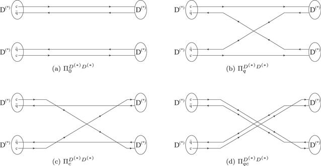
Figure 12. Feynman diagrams between two charmed mesons corresponding to: (a) the leading term ${{\rm{\Pi }}}_{0}^{{D}^{(* )}{D}^{(* )}}(x)={{\rm{\Pi }}}^{{D}^{(* )}}(x)\times {{\rm{\Pi }}}^{{D}^{(* )}}(x)$ contributed by two non-correlated charmed mesons, (b) the light-quark-exchange interaction ${{\rm{\Pi }}}_{q}^{{D}^{(* )}{D}^{(* )}}$, (c) the heavy-quark-exchange interaction ${{\rm{\Pi }}}_{c}^{{D}^{(* )}{D}^{(* )}}$, and (d) the interaction ${{\rm{\Pi }}}_{{qc}}^{{D}^{(* )}{D}^{(* )}}$ exchanging both light and heavy quarks. Here q denotes a light up/down quark.
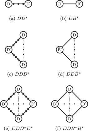
Figure 13. Illustration of the hadronic molecules DD* and $D{\bar{B}}^{* }$ of (I)JP = (0)1+, DDD* and ${DD}{\bar{B}}^{* }$ of (I)JP = (1/2)1+, and DDD*D* and ${DD}{\bar{B}}^{* }{\bar{B}}^{* }$ of (I)JP = (0)0+/(0)2+ in our model.
The (I)JP = (0)1+ DD* hadronic molecule contains two shared light antiquarks with the configuration of (I)JP = (0)1+:
color flavor spin orbital total
${\bar{q}}_{1}\leftrightarrow {\bar{q}}_{2}$ S A S S A
We estimate its binding energy to be
$\begin{eqnarray}{B}_{I=0,J=1}^{{{DD}}^{* }}=A-R-2\epsilon \sim 1\,\mathrm{MeV},\end{eqnarray}$
suggesting it possible to interpret the recently observed ${T}_{{cc}}^{+}$ [44, 45] as the (I)JP = (0)1+ DD* covalent hadronic molecule.
The (I)JP = (0)1+ ${D}^{* }{D}^{* }/\bar{B}{\bar{B}}^{* }/{\bar{B}}^{* }{\bar{B}}^{* }$ hadronic molecules have similar binding energies:
$\begin{eqnarray}{B}_{I=0,J=1}^{{D}^{* }{D}^{* }/\bar{B}{\bar{B}}^{* }/{\bar{B}}^{* }{\bar{B}}^{* }}=A-R-2\epsilon \sim 1\,\mathrm{MeV}.\end{eqnarray}$
However, in the above estimations we have not considered the spin splitting effect, and we have also not considered the long-range light-meson-exchange interaction. These uncertainties prevent us to well determine whether these hadronic molecules exist or not.
Different from D(*)D(*) and ${\bar{B}}^{(* )}{\bar{B}}^{(* )}$ molecules, the charm and bottom quarks in ${D}^{(* )}{\bar{B}}^{(* )}$ hadronic molecules can not be exchanged, so they are not capable of forming repulsive cores, i.e. there does not exist the Feynman diagram corresponding to figure 12(c). In this case we include the spin splitting effect described by the parameter κ, and estimate binding energies of ${D}^{(* )}{\bar{B}}^{(* )}$ hadronic molecules to be
$\begin{eqnarray}\begin{array}{rcl}{B}_{I=0,J=0}^{D\bar{B}} & = & A-2\epsilon -1.33\kappa \sim 1\,\mathrm{MeV},\\ {B}_{I=0,J=1}^{D{\bar{B}}^{* }/{D}^{* }\bar{B}} & = & A-2\epsilon +0.44\kappa \sim 24\,\mathrm{MeV},\\ {B}_{I=0,J=0}^{{D}^{* }{\bar{B}}^{* }} & = & A-2\epsilon -1.33\kappa \sim 1\,\mathrm{MeV},\\ {B}_{I=0,J=1}^{{D}^{* }{\bar{B}}^{* }} & = & A-2\epsilon +4\kappa \sim 70\,\mathrm{MeV},\\ {B}_{I=0,J=2}^{{D}^{* }{\bar{B}}^{* }} & = & A-2\epsilon -1.33\kappa \sim 1\,\mathrm{MeV}.\end{array}\end{eqnarray}$
Especially, binding energies of the (I)JP = (0)1+ $D{\bar{B}}^{* }/{D}^{* }\bar{B}$ covalent hadronic molecules are much larger than those of the (I)JP = (0)1+ ${{DD}}^{* }/\bar{B}{\bar{B}}^{* }$ molecules.
In the above estimations we have assumed that the charm and bottom quarks form the symmetric color representation 6c, so that
$\begin{eqnarray}\langle {\lambda }_{c}\cdot {\lambda }_{b}\rangle =\displaystyle \frac{16}{3}.\end{eqnarray}$
Besides, we need to perform the spin decomposition from the $\left|{s}_{c\bar{q}},{s}_{b{\bar{q}}^{{\prime} }};J\right\rangle $ basis to the $\left|{s}_{{cb}},{s}_{\bar{q}{\bar{q}}^{{\prime} }};J\right\rangle $ basis (see appendix B), and select the components satisfying ${s}_{\bar{q}{\bar{q}}^{{\prime} }}=1$ to evaluate ⟨sc · sb⟩. Take the (I)JP = (0)1+ $D{\bar{B}}^{* }$ molecule as an example, we obtain
$\begin{eqnarray}\begin{array}{l}\langle {0}_{c\bar{q}},{1}_{b{\bar{q}}^{{\prime} }};1| {s}_{c}\cdot {s}_{b}\left|{0}_{c\bar{q}},{1}_{b{\bar{q}}^{{\prime} }};1\right\rangle \\ \quad \to \displaystyle \frac{4}{3}\times \left(\displaystyle \frac{1}{4}\langle {0}_{{cb}},{1}_{\bar{q}{\bar{q}}^{{\prime} }};1| {s}_{c}\cdot {s}_{b}| {0}_{{cb}},{1}_{\bar{q}{\bar{q}}^{{\prime} }};1\rangle \right.\\ \quad \left.+\displaystyle \frac{1}{2}\langle {1}_{{cb}},{1}_{\bar{q}{\bar{q}}^{{\prime} }};1| {s}_{c}\cdot {s}_{b}| {1}_{{cb}},{1}_{\bar{q}{\bar{q}}^{{\prime} }};1\rangle \right)\\ \quad =-0.0833.\end{array}\end{eqnarray}$
We further use D(*) to compose multi-D(*) hadronic molecules, such as the DDD* and DDD*D* molecules, etc. As illustrated in figures 13(c), (e), their structures are similar to the 3He and 4He, respectively. We estimate their binding energies to be:
$\begin{eqnarray}\begin{array}{rcl}{B}_{I=1/2,J=1}^{{{DDD}}^{* }} & = & 2A-2R-3\epsilon \sim 8\,\mathrm{MeV},\\ {B}_{I=0,J=0,2}^{{{DDD}}^{* }{D}^{* }} & = & 4A-4R-4\epsilon \sim 28\,\mathrm{MeV}.\end{array}\end{eqnarray}$
Besides, our model supports the existence of the ${DD}{\bar{B}}^{* }$ and ${DD}{\bar{B}}^{* }{\bar{B}}^{* }$ hadronic molecules, etc. As illustrated in figures 13(d), (f), they have much larger binding energies:
$\begin{eqnarray}\begin{array}{rcl}{B}_{I=1/2,J=1}^{{DD}{\bar{B}}^{* }} & = & 2A-3\epsilon +0.89\kappa \sim 54\,\mathrm{MeV},\\ {B}_{I=0,J=0,2}^{{DD}{\bar{B}}^{* }{\bar{B}}^{* }} & = & 4A-4\epsilon +1.78\kappa \sim 119\,\mathrm{MeV}.\end{array}\end{eqnarray}$
More examples can be found in table 2.
Table 2. Binding energies of some possibly-existing covalent hadronic molecules, estimated in our toy model through the simplified formula B = NAA + NSSNRRNε, with A ∼ 30 MeV, S ∼ 20 MeV, R ∼ 17 MeV, and ε ∼ 6 MeV. We do not take into account the spin splitting effect described by the parameter κ ∼ 13 MeV here.
Molecules Binding energies Molecules Binding energies
2H, ${D}^{* }{D}^{(* )}/{\bar{B}}^{* }{\bar{B}}^{(* )}$ 1 MeV ${D}^{(* )}{\bar{B}}^{(* )}$ 18 MeV
3H/3He, ${D}^{* }{D}^{(* )}{D}^{(* )}/{\bar{B}}^{* }{\bar{B}}^{(* )}{\bar{B}}^{(* )}$ 8 MeV ${D}^{(* )}{D}^{(* )}{\bar{B}}^{(* )}/{D}^{(* )}{\bar{B}}^{(* )}{\bar{B}}^{(* )}$ 42 MeV
4He, ${D}^{* }{D}^{* }{D}^{(* )}{D}^{(* )}/{\bar{B}}^{* }{\bar{B}}^{* }{\bar{B}}^{(* )}{\bar{B}}^{(* )}$ 28 MeV ${D}^{* }{D}^{(* )}{D}^{(* )}{\bar{B}}^{(* )}/{D}^{(* )}{\bar{B}}^{(* )}{\bar{B}}^{(* )}{\bar{B}}^{* }$ 62 MeV
${D}^{(* )}{D}^{(* )}{\bar{B}}^{(* )}{\bar{B}}^{(* )}$ 96 MeV
${{\rm{\Sigma }}}_{c}^{(* )}{{\rm{\Sigma }}}_{c}^{(* )}/{{\rm{\Sigma }}}_{b}^{(* )}{{\rm{\Sigma }}}_{b}^{(* )}$ 31 MeV ${{\rm{\Sigma }}}_{c}^{(* )}{{\rm{\Sigma }}}_{b}^{(* )}$ 48 MeV
${\bar{D}}^{(* )}{{\rm{\Sigma }}}_{c}^{(* )}/{\bar{D}}^{(* )}{{\rm{\Sigma }}}_{b}^{(* )}/{B}^{(* )}{{\rm{\Sigma }}}_{c}^{(* )}/{B}^{(* )}{{\rm{\Sigma }}}_{b}^{(* )}$ 18 MeV
${\bar{D}}^{(* )}{\bar{D}}^{(* )}{{\rm{\Sigma }}}_{c}^{(* )}$ 42 MeV
${D}^{(* )}{\bar{B}}_{s}^{(* )}$ 8 MeV
${}_{{\rm{\Lambda }}}^{3}$H, ${D}^{* }{D}^{(* )}{D}_{s}^{(* )}$ 1 MeV ${D}^{(* )}{D}^{(* )}{\bar{B}}_{s}^{(* )}$ 35 MeV
${}_{{\rm{\Lambda }}}^{4}$H/${}_{{\rm{\Lambda }}}^{4}$He, ${D}^{* }{D}^{(* )}{D}^{(* )}{D}_{s}^{(* )}$ 11 MeV ${D}^{* }{D}^{(* )}{D}^{(* )}{\bar{B}}_{s}^{(* )}$ 62 MeV
${}_{{\rm{\Lambda }}}^{5}$He, ${D}^{* }{D}^{* }{D}^{(* )}{D}^{(* )}{D}_{s}^{(* )}$ 31 MeV ${D}^{* }{D}^{* }{D}^{(* )}{D}^{(* )}{\bar{B}}_{s}^{(* )}$ 82 MeV
${}_{{\rm{\Lambda }}{\rm{\Lambda }}}^{\,\,6}$He, ${D}^{* }{D}^{* }{D}^{(* )}{D}^{(* )}{D}_{s}^{(* )}{D}_{s}^{(* )}$ 34 MeV ${D}^{* }{D}^{* }{D}^{(* )}{D}^{(* )}{\bar{B}}_{s}^{(* )}{\bar{B}}_{s}^{(* )}$ 136 MeV
${{\rm{\Sigma }}}_{c}^{(* )}{{\rm{\Xi }}}_{c}^{(^{\prime} * )}$ 21 MeV ${{\rm{\Sigma }}}_{c}^{(* )}{{\rm{\Xi }}}_{b}^{(^{\prime} * )}$ 38 MeV
${{\rm{\Xi }}}_{c}^{(^{\prime} * )}{{\rm{\Xi }}}_{c}^{(^{\prime} * )}$ 11 MeV ${{\rm{\Xi }}}_{c}^{(^{\prime} * )}{{\rm{\Xi }}}_{b}^{(^{\prime} * )}$ 28 MeV
${{\rm{\Sigma }}}_{c}^{(* )}{{\rm{\Xi }}}_{c}^{(^{\prime} * )}{{\rm{\Xi }}}_{c}^{(^{\prime} * )}$ 71 MeV ${{\rm{\Sigma }}}_{c}^{(* )}{{\rm{\Xi }}}_{c}^{(^{\prime} * )}{{\rm{\Xi }}}_{b}^{(^{\prime} * )}$ 105 MeV
${\bar{D}}^{(* )}{{\rm{\Xi }}}_{c}^{(^{\prime} * )}$ 18 MeV
${\bar{D}}^{(* )}{\bar{D}}^{(* )}{{\rm{\Xi }}}_{c}^{(^{\prime} * )}$ 35 MeV
${\bar{D}}^{(* )}{\bar{D}}^{(* )}{{\rm{\Xi }}}_{c}^{(^{\prime} * )}{{\rm{\Xi }}}_{b}^{(^{\prime} * )}$ 116 MeV

6.4. ${{\rm{\Sigma }}}_{c}^{(* )}{{\rm{\Sigma }}}_{c}^{(* )}/{{\rm{\Sigma }}}_{c}^{(* )}{{\rm{\Sigma }}}_{b}^{(* )}/{{\rm{\Sigma }}}_{b}^{(* )}{{\rm{\Sigma }}}_{b}^{(* )}$ molecules

We follow section 6.3 and find that the two charm quarks in ${{\rm{\Sigma }}}_{c}^{(* )}{{\rm{\Sigma }}}_{c}^{(* )}$ hadronic molecules also form repulsive cores. Accordingly, we can estimate binding energies of ${{\rm{\Sigma }}}_{c}^{(* )}{{\rm{\Sigma }}}_{c}^{(* )}/{{\rm{\Sigma }}}_{b}^{(* )}{{\rm{\Sigma }}}_{b}^{(* )}$ hadronic molecules, as illustrated in figure 14(a).
Figure 14. Illustration of the hadronic molecules ${{\rm{\Sigma }}}_{c}{{\rm{\Sigma }}}_{c}^{* }$ and ${{\rm{\Sigma }}}_{c}{{\rm{\Sigma }}}_{b}^{* }$ of (I)JP = (0)1+/(0)2+ in our model.
The (I)JP = (0)1+ ${{\rm{\Sigma }}}_{c}[{q}_{1}{q}_{2}c]{{\rm{\Sigma }}}_{c}[{q}_{3}{q}_{4}{c}^{{\prime} }]$ hadronic molecule contains four shared light up/down quarks with the configuration of (I)JP = (0)2+:
color flavor spin orbital total
q1q3 S A S S A
q2q4 S A S S A
q1q2 A S S S A
q1q4 A S S S A
q2q3 A S S S A
q3q4 A S S S A
We estimate its binding energy to be
$\begin{eqnarray}{B}_{I=0,J=1}^{{{\rm{\Sigma }}}_{c}{{\rm{\Sigma }}}_{c}}=2A-R-2\epsilon \sim 31\,\mathrm{MeV}.\end{eqnarray}$
The I = 0 ${{\rm{\Sigma }}}_{c}{{\rm{\Sigma }}}_{c}^{* }/{{\rm{\Sigma }}}_{c}^{* }{{\rm{\Sigma }}}_{c}^{* }$ hadronic molecules have similar binding energies:
$\begin{eqnarray}{B}_{I=0}^{{{\rm{\Sigma }}}_{c}{{\rm{\Sigma }}}_{c}^{* }/{{\rm{\Sigma }}}_{c}^{* }{{\rm{\Sigma }}}_{c}^{* }}=2A-R-2\epsilon \sim 31\,\mathrm{MeV}.\end{eqnarray}$
So do their corresponding ${{\rm{\Sigma }}}_{b}^{(* )}{{\rm{\Sigma }}}_{b}^{(* )}$ hadronic molecules. However, the (I)JP = (0)0+ ${{\rm{\Sigma }}}_{c}{{\rm{\Sigma }}}_{c}/{{\rm{\Sigma }}}_{c}^{* }{{\rm{\Sigma }}}_{c}^{* }$ and ${{\rm{\Sigma }}}_{b}{{\rm{\Sigma }}}_{b}/{{\rm{\Sigma }}}_{b}^{* }{{\rm{\Sigma }}}_{b}^{* }$ hadronic molecules do not exist due to the Fermi–Dirac statistics.
Different from ${{\rm{\Sigma }}}_{c}^{(* )}{{\rm{\Sigma }}}_{c}^{(* )}$ and ${{\rm{\Sigma }}}_{b}^{(* )}{{\rm{\Sigma }}}_{b}^{(* )}$ molecules, the charm and bottom quarks in ${{\rm{\Sigma }}}_{c}^{(* )}{{\rm{\Sigma }}}_{b}^{(* )}$ hadronic molecules can not be exchanged, so they are not capable of forming repulsive cores. In this case we include the spin splitting effect described by the parameter κ, and estimate binding energies of ${{\rm{\Sigma }}}_{c}^{(* )}{{\rm{\Sigma }}}_{b}^{(* )}$ hadronic molecules to be
$\begin{eqnarray}\begin{array}{rcl}{B}_{I=0,J=1}^{{{\rm{\Sigma }}}_{c}{{\rm{\Sigma }}}_{b}} & = & 2A-2\epsilon -1.33\kappa \sim 31\,\mathrm{MeV},\\ {B}_{I=0,J=1}^{{{\rm{\Sigma }}}_{c}{{\rm{\Sigma }}}_{b}^{* }/{{\rm{\Sigma }}}_{c}^{* }{{\rm{\Sigma }}}_{b}} & = & 2A-2\epsilon -1.33\kappa \sim 31\,\mathrm{MeV},\\ {B}_{I=0,J=2}^{{{\rm{\Sigma }}}_{c}{{\rm{\Sigma }}}_{b}^{* }/{{\rm{\Sigma }}}_{c}^{* }{{\rm{\Sigma }}}_{b}} & = & 2A-2\epsilon +0.8\kappa \sim 58\,\mathrm{MeV},\\ {B}_{I=0,J=1}^{{{\rm{\Sigma }}}_{c}^{* }{{\rm{\Sigma }}}_{b}^{* }} & = & 2A-2\epsilon -1.33\kappa \sim 31\,\mathrm{MeV},\\ {B}_{I=0,J=2}^{{{\rm{\Sigma }}}_{c}^{* }{{\rm{\Sigma }}}_{b}^{* }} & = & 2A-2\epsilon +4\kappa \sim 100\,\mathrm{MeV},\\ {B}_{I=0,J=3}^{{{\rm{\Sigma }}}_{c}^{* }{{\rm{\Sigma }}}_{b}^{* }} & = & 2A-2\epsilon -1.33\kappa \sim 31\,\mathrm{MeV}.\end{array}\end{eqnarray}$

6.5. ${\bar{D}}^{(* )}{{\rm{\Sigma }}}_{c}^{(* )}/{\bar{D}}^{(* )}{{\rm{\Sigma }}}_{b}^{(* )}/{B}^{(* )}{{\rm{\Sigma }}}_{c}^{(* )}/{B}^{(* )}{{\rm{\Sigma }}}_{b}^{(* )}$ molecules

The charm and anti-charm quarks in ${\bar{D}}^{(* )}{{\rm{\Sigma }}}_{c}^{(* )}$ hadronic molecules can not be exchanged, so they are not capable of forming repulsive cores. Accordingly, we include the spin splitting effect described by the parameter κ, and estimate their binding energies to be
$\begin{eqnarray}\begin{array}{rcl}{B}_{I=1/2,J=1/2}^{\bar{D}{{\rm{\Sigma }}}_{c}} & = & A-2\epsilon -0.67\kappa \sim 9\,\mathrm{MeV},\\ {B}_{I=1/2,J=3/2}^{\bar{D}{{\rm{\Sigma }}}_{c}^{* }} & = & A-2\epsilon +0.33\kappa \sim 22\,\mathrm{MeV},\\ {B}_{I=1/2,J=1/2}^{{\bar{D}}^{* }{{\rm{\Sigma }}}_{c}} & = & A-2\epsilon -0.67\kappa \sim 9\,\mathrm{MeV},\\ {B}_{I=1/2,J=3/2}^{{\bar{D}}^{* }{{\rm{\Sigma }}}_{c}} & = & A-2\epsilon +0.33\kappa \sim 22\,\mathrm{MeV},\\ {B}_{I=1/2,J=1/2}^{{\bar{D}}^{* }{{\rm{\Sigma }}}_{c}^{* }} & = & A-2\epsilon -0.67\kappa \sim 9\,\mathrm{MeV},\\ {B}_{I=1/2,J=3/2}^{{\bar{D}}^{* }{{\rm{\Sigma }}}_{c}^{* }} & = & A-2\epsilon +1.83\kappa \sim 42\,\mathrm{MeV},\\ {B}_{I=1/2,J=5/2}^{{\bar{D}}^{* }{{\rm{\Sigma }}}_{c}^{* }} & = & A-2\epsilon -0.67\kappa \sim 9\,\mathrm{MeV}.\end{array}\end{eqnarray}$
Similarly, we can estimate binding energies of ${\bar{D}}^{(* )}{{\rm{\Sigma }}}_{b}^{(* )}/{B}^{(* )}{{\rm{\Sigma }}}_{c}^{(* )}/{B}^{(* )}{{\rm{\Sigma }}}_{b}^{(* )}$ hadronic molecules, which are the same as their corresponding ${\bar{D}}^{(* )}{{\rm{\Sigma }}}_{c}^{(* )}$ ones.
These hadronic molecules all contain three shared light up/down quarks with the configuration of (I)JP = (1/2)3/2+:
color flavor spin orbital total
q1q2 S A S S A
q1q3 A S S S A
q2q3 A S S S A
We further use two charmed mesons and one ${{\rm{\Sigma }}}_{c}^{(* )}$ baryon to compose ${\bar{D}}^{(* )}{\bar{D}}^{(* )}{{\rm{\Sigma }}}_{c}^{(* )}$ hadronic molecules. Especially, the $\bar{D}[\bar{c}{q}_{1}]\bar{D}[{\bar{c}}^{{\prime} }{q}_{2}]{{\rm{\Sigma }}}_{c}[{q}_{3}{q}_{4}c]$ illustrated in figure 15(b) contains four shared light up/down quarks with the configuration of (I)JP = (0)2+:
color flavor spin orbital total
q1q3 S A S S A
q2q4 S A S S A
q1q2 A S S S A
q1q4 A S S S A
q2q3 A S S S A
q3q4 A S S S A
We estimate its binding energy to be:
$\begin{eqnarray}{B}_{I=0,J=1/2}^{\bar{D}\bar{D}{{\rm{\Sigma }}}_{c}}=2A-3\epsilon -1.33\kappa \sim 25\,\mathrm{MeV}.\end{eqnarray}$
More examples can be found in table 2.
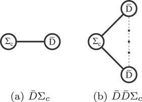
Figure 15. Illustration of the hadronic molecules $\bar{D}{{\rm{\Sigma }}}_{c}$ of (I)JP = (1/2)1/2 and $\bar{D}\bar{D}{{\rm{\Sigma }}}_{c}$ of (I)JP = (0)1/2+ in our model.

6.6. Molecules with strangeness

In the previous subsections we only consider the up and down quarks as exchanged light quarks, and in this subsection we further take the light strange quark into account. We introduce another parameter S to describe the attractive interaction induced by the shared strange and up/down quarks with the configuration of either (I)JP = (1/2)0+ or (1/2)1+:
color flavor spin orbital total
sq S S A S A
sq S A S S A
This parameter is estimated to be S ∼ 20 MeV for each bond, with NS the number of such bonds. We still use the solid curve to illustrate it, but this solid curve is slightly thinner than that denoting the attractive bond A.
Taking the Λ hyperon as the combination of an (I)JP = (0)0+ up–down quark pair together with a strange quark, we can estimate binding energies of some hypernuclei. Considering that there are at most two up, two down, and two strange quarks in the lowest orbit, we obtain:
$\begin{eqnarray}\begin{array}{rcl}{B}_{I=0}^{{}_{{\rm{\Lambda }}}^{3}{\rm{H}}} & = & A+2S-3R-3\epsilon \sim 1\,\mathrm{MeV},\\ {B}_{I=1/2}^{{}_{{\rm{\Lambda }}}^{4}{\rm{H}}{/}_{{\rm{\Lambda }}}^{4}\mathrm{He}} & = & 2A+3S-5R-4\epsilon \sim 11\,\mathrm{MeV},\\ {B}_{I=0}^{{}_{{\rm{\Lambda }}}^{5}\mathrm{He}} & = & 4A+3S-7R-5\epsilon \sim 31\,\mathrm{MeV},\\ {B}_{I=0}^{{}_{{\rm{\Lambda }}{\rm{\Lambda }}}^{\,\,6}\mathrm{He}} & = & 4A+6S-10R-6\epsilon \sim 34\,\mathrm{MeV}.\end{array}\end{eqnarray}$
We illustrate these hypernuclei in figure 16. More possibly-existing covalent hadronic molecules with strangeness can be found in table 2.
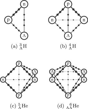
Figure 16. Illustration of the ${}_{{\rm{\Lambda }}}^{3}$H, ${}_{{\rm{\Lambda }}}^{4}$H, ${}_{{\rm{\Lambda }}}^{5}$He, and ${}_{{\rm{\Lambda }}{\rm{\Lambda }}}^{\,\,6}$He in our model. The shape of ppnn in the subfigures (c) and (d) is a tetrahedron other than a square.

6.7. Discussions on the spin splitting effect

In the present study we investigate the spin splitting effect through equations (91) and (92) with the same parameter κ ∼ 13 MeV. These two equations are used for ${\bar{D}}^{(* )}{{\rm{\Sigma }}}_{c}^{(* )}$ and ${D}^{(* )}{\bar{B}}^{(* )}/{{\rm{\Sigma }}}_{c}^{(* )}{{\rm{\Sigma }}}_{b}^{(* )}$ hadronic molecules, respectively; while we do not include such terms when investigating ${D}^{(* )}{D}^{(* )}/{{\rm{\Sigma }}}_{c}^{(* )}{{\rm{\Sigma }}}_{c}^{(* )}$ hadronic molecules, since the interaction between two charm quarks has been (partly) taken into account in the repulsive bond energy R.
Because we do not well understand the spin splitting effect in hadronic molecules at this moment, we still need to update it with future experiments, and there can be other approaches that better describe it. We take ${\bar{D}}^{(* )}{{\rm{\Sigma }}}_{c}^{(* )}$ hadronic molecules as an example, and discuss several possible improvements.
Firstly, it is possible to use two different κ's for equations (91) and (92). It is also possible to use some formulae other than equations (91) and (92), such as the spin–spin interaction
$\begin{eqnarray}{ \mathcal H }{{\prime\prime} }_{\,{\rm{spin}}}=-{\kappa }^{{\prime} }\,\langle {s}_{{\bar{D}}^{(* )}}\cdot {s}_{{{\rm{\Sigma }}}_{c}^{(* )}}\rangle ,\end{eqnarray}$
or the spin–orbit interaction, etc.
Secondly, in the present study we perform the spin decomposition from the ${\left|{s}_{\bar{c}{q}_{1}},{s}_{{q}_{2}{q}_{3}c};J\right\rangle }_{{s}_{{q}_{2}{q}_{3}}=1}$ basis to the ${\left|{s}_{\bar{c}c},{s}_{{q}_{1}{q}_{2}{q}_{3}};J\right\rangle }_{{s}_{{q}_{2}{q}_{3}}=1}$ basis, and select the components satisfying ${s}_{{q}_{1}{q}_{2}{q}_{3}}=3/2$ to evaluate $\langle {s}_{c}\cdot {s}_{\bar{c}}\rangle $. This is because the three light up/down quarks of (I)JP = (1/2)3/2+ are assumed to supply the attraction forming ${\bar{D}}^{(* )}{{\rm{\Sigma }}}_{c}^{(* )}$ hadronic molecules in our model, while the two heavy quarks $c/\bar{c}$ are assumed to be freely polarised. If this is not the case and $c/\bar{c}$ are also fully polarised, there might be two $\bar{D}{{\rm{\Sigma }}}_{c}^{* }$ hadronic molecules with either ${s}_{\bar{c}c}=0$ or ${s}_{\bar{c}c}=1$ (see appendix B):
$\begin{eqnarray}\begin{array}{rcl}{\left|{s}_{\bar{c}{q}_{1}},{s}_{{q}_{2}{q}_{3}c};J\right\rangle }_{{s}_{{q}_{2}{q}_{3}}=1} & \to & {\left|{s}_{\bar{c}c},{s}_{{q}_{1}{q}_{2}{q}_{3}};J\right\rangle }_{{s}_{{q}_{2}{q}_{3}}=1},\\ \left|0,\displaystyle \frac{3}{2};\displaystyle \frac{3}{2}\right\rangle & \to & \left|0,\displaystyle \frac{3}{2};\displaystyle \frac{3}{2}\right\rangle ,\end{array}\end{eqnarray}$
$\begin{eqnarray}\left|0,\displaystyle \frac{3}{2};\displaystyle \frac{3}{2}\right\rangle \to \left|1,\displaystyle \frac{3}{2};\displaystyle \frac{3}{2}\right\rangle .\end{eqnarray}$
It can be seen from the recent LHCb experiment [6] that there might be two peaks near the $\bar{D}{{\rm{\Sigma }}}_{c}^{* }$ threshold, and we propose to further study them as well as the ${P}_{c}{\left(4440\right)}^{+}$ and ${P}_{c}{\left(4457\right)}^{+}$ in order to better understand the spin splitting effect of hadronic molecules in future experiments.
To end this section, we further simplify our toy model by neglecting the spin splitting effect described by the parameter κ ∼ 13 MeV, and estimate binding energies of some possibly-existing covalent hadronic molecules through the simplified formula,
$\begin{eqnarray}B={N}_{A}A+{N}_{S}S-{N}_{R}R-N\epsilon ,\end{eqnarray}$
which still have four parameters A ∼ 30 MeV, S ∼ 20 MeV, R ∼ 17 MeV, and ε ∼ 6 MeV. The obtained results are summarized in table 2,
Very quickly, we arrive at the unique feature of our covalent hadronic molecule picture: binding energies of the (I)JP = (0)1+ $D{\bar{B}}^{* }/{D}^{* }\bar{B}$ hadronic molecules are much larger than those of the (I)JP = (0)1+ ${{DD}}^{* }/\bar{B}{\bar{B}}^{* }$ ones, while the (I)JP = (1/2)1/2+ $\bar{D}{{\rm{\Sigma }}}_{c}/\bar{D}{{\rm{\Sigma }}}_{b}/B{{\rm{\Sigma }}}_{c}/B{{\rm{\Sigma }}}_{b}$ hadronic molecules have similar binding energies. This is due to the two identical heavy quarks in ${{DD}}^{* }/\bar{B}{\bar{B}}^{* }$ hadronic molecules forming repulsive cores, but the two different heavy quarks in $D{\bar{B}}^{* }/{D}^{* }\bar{B}$ and $\bar{D}{{\rm{\Sigma }}}_{c}/\bar{D}{{\rm{\Sigma }}}_{b}/B{{\rm{\Sigma }}}_{c}/B{{\rm{\Sigma }}}_{b}$ hadronic molecules do not.

7. Summary and discussions

In this paper we systematically examine Feynman diagrams corresponding to the ${\bar{D}}^{(* )}{{\rm{\Sigma }}}_{c}^{(* )}$, ${\bar{D}}^{(* )}{{\rm{\Lambda }}}_{c}$, ${D}^{(* )}{\bar{K}}^{* }$, and ${D}^{(* )}{\bar{D}}^{(* )}$ hadronic molecular states. Take the $\bar{D}{{\rm{\Sigma }}}_{c}$ molecule as an example, first we calculate correlation functions of $\bar{D}$ and Σc in the coordinate space to be ${{\rm{\Pi }}}^{\bar{D}}(x)$ and ${{\rm{\Pi }}}^{{{\rm{\Sigma }}}_{c}}(x)$, respectively. Then we calculate correlation functions of the ${D}^{-}{{\rm{\Sigma }}}_{c}^{++}$, ${\bar{D}}^{0}{{\rm{\Sigma }}}_{c}^{+}$, I = 1/2 $\bar{D}{{\rm{\Sigma }}}_{c}$, and I = 3/2 $\bar{D}{{\rm{\Sigma }}}_{c}$ molecules, separated into:
$\begin{eqnarray*}\begin{array}{rcl}{{\rm{\Pi }}}^{{D}^{-}{{\rm{\Sigma }}}_{c}^{++}}(x) & = & {{\rm{\Pi }}}_{0}^{\bar{D}{{\rm{\Sigma }}}_{c}}(x)+{{\rm{\Pi }}}_{G}^{\bar{D}{{\rm{\Sigma }}}_{c}}(x),\\ {{\rm{\Pi }}}^{{\bar{D}}^{0}{{\rm{\Sigma }}}_{c}^{+}}(x) & = & {{\rm{\Pi }}}_{0}^{\bar{D}{{\rm{\Sigma }}}_{c}}(x)+{{\rm{\Pi }}}_{G}^{\bar{D}{{\rm{\Sigma }}}_{c}}(x)-{{\rm{\Pi }}}_{Q}^{\bar{D}{{\rm{\Sigma }}}_{c}}(x),\\ {{\rm{\Pi }}}_{I=1/2}^{\bar{D}{{\rm{\Sigma }}}_{c}}(x) & = & {{\rm{\Pi }}}_{0}^{\bar{D}{{\rm{\Sigma }}}_{c}}(x)+{{\rm{\Pi }}}_{G}^{\bar{D}{{\rm{\Sigma }}}_{c}}(x)+{{\rm{\Pi }}}_{Q}^{\bar{D}{{\rm{\Sigma }}}_{c}}(x),\\ {{\rm{\Pi }}}_{I=3/2}^{\bar{D}{{\rm{\Sigma }}}_{c}}(x) & = & {{\rm{\Pi }}}_{0}^{\bar{D}{{\rm{\Sigma }}}_{c}}(x)+{{\rm{\Pi }}}_{G}^{\bar{D}{{\rm{\Sigma }}}_{c}}(x)-2{{\rm{\Pi }}}_{Q}^{\bar{D}{{\rm{\Sigma }}}_{c}}(x),\end{array}\end{eqnarray*}$
where ${{\rm{\Pi }}}_{0}^{\bar{D}{{\rm{\Sigma }}}_{c}}(x)={{\rm{\Pi }}}^{\bar{D}}(x)\times {{\rm{\Pi }}}^{{{\rm{\Sigma }}}_{c}}(x)$ is the leading term contributed by non-correlated $\bar{D}$ and Σc; ${{\rm{\Pi }}}_{G}^{\bar{D}{{\rm{\Sigma }}}_{c}}$ describes the double-gluon-exchange interaction between them, but we do not take it into account in the present study, because the other term ${{\rm{\Pi }}}_{Q}^{\bar{D}{{\rm{\Sigma }}}_{c}}$ is much larger.
The term ${{\rm{\Pi }}}_{Q}^{\bar{D}{{\rm{\Sigma }}}_{c}}$ describes the light-quark-exchange effect between $\bar{D}$ and Σc, i.e. $\bar{D}$ and Σc are exchanging and so sharing light up/down quarks. We systematically study it using the method of QCD sum rules, and calculate the mass correction ΔM induced by this term. Note that the obtained results can be further applied to study the production and decay properties of these hadronic molecular states [6870]. The parameter ΔM is actually not the binding energy, because we are using local currents in QCD sum rule analyses. We can relate it to some potential V(r) between $\bar{D}$ and Σc induced by exchanged/shared light quarks, satisfying:
$\begin{eqnarray*}\begin{array}{rcl}V(| r| =0) & = & {\rm{\Delta }}M,\\ V(| r| \to \infty ) & \to & 0.\end{array}\end{eqnarray*}$
We systematically investigate the light-quark-exchange term ΠQ, and study its contributions to the ${\bar{D}}^{(* )}{{\rm{\Sigma }}}_{c}^{(* )}$, ${\bar{D}}^{(* )}{{\rm{\Lambda }}}_{c}$, ${D}^{(* )}{\bar{K}}^{* }$, and ${D}^{(* )}{\bar{D}}^{(* )}$ hadronic molecular states. We calculate their mass corrections, some of which are listed here:
$\begin{eqnarray*}\begin{array}{rcl}{\rm{\Delta }}{M}_{I=1/2,J=1/2}^{\bar{D}{{\rm{\Sigma }}}_{c}} & = & -95\,\mathrm{MeV},\\ {\rm{\Delta }}{M}_{I=1/2,J=3/2}^{{\bar{D}}^{* }{{\rm{\Sigma }}}_{c}} & = & -89\,\mathrm{MeV},\\ {\rm{\Delta }}{M}_{I=1/2,J=3/2}^{\bar{D}{{\rm{\Sigma }}}_{c}^{* }} & = & -86\,\mathrm{MeV},\\ {\rm{\Delta }}{M}_{I=1/2,J=5/2}^{{\bar{D}}^{* }{{\rm{\Sigma }}}_{c}^{* }} & = & -107\,\mathrm{MeV},\\ {\rm{\Delta }}{M}_{I=0,J=1}^{D{\bar{K}}^{* }} & = & -180\,\mathrm{MeV},\\ {\rm{\Delta }}{M}_{I=0,J=2}^{{D}^{* }{\bar{K}}^{* }} & = & -119\,\mathrm{MeV}.\end{array}\end{eqnarray*}$
These results suggest their corresponding light-quark-exchange potentials V(r) to be attractive, so there can be

the $\bar{D}{{\rm{\Sigma }}}_{c}$ covalent molecule of I = 1/2 and J = 1/2,

the ${\bar{D}}^{* }{{\rm{\Sigma }}}_{c}$ covalent molecule of I = 1/2 and J = 3/2,

the $\bar{D}{{\rm{\Sigma }}}_{c}^{* }$ covalent molecule of I = 1/2 and J = 3/2,

the ${\bar{D}}^{* }{{\rm{\Sigma }}}_{c}^{* }$ covalent molecule of I = 1/2 and J = 5/2,

the $D{\bar{K}}^{* }$ covalent molecule of I = 0 and J = 1,

the ${D}^{* }{\bar{K}}^{* }$ covalent molecule of I = 0 and J = 2.

The binding mechanism induced by shared light quarks is somewhat similar to the covalent bond in chemical molecules induced by shared electrons, so we call such hadronic molecules ‘covalent hadronic molecules'. Different from the chemical molecules, the internal structure of the hadrons and so the covalent hadronic molecules is much more complicated, since they contain not only the valence quarks but also the sea quarks and gluons. In the present study we consider the covalent hadronic molecules induced only by the shared valence quarks.
Recalling that the two shared electrons must spin in opposite directions (and so totally antisymmetric obeying the Pauli principle) in order to form a chemical covalent bond, our QCD sum rule results indicate a similar hypothesis: the light-quark-exchange interaction is attractive when the shared light quarks are totally antisymmetric so that obey the Pauli principle.
Its logical chain is quite straightforward. We assume the two light quarks qA inside Y and qB inside Z are totally antisymmetric. Hence, qA and qB obey the Pauli principle, so that they can be exchanged and shared. By doing this, wave-functions of Y and Z overlap with each other, so that they are attracted and there can be a covalent hadronic molecule $X=\left|{YZ}\right\rangle $. This picture has been depicted in figure 2. We believe it is better and more important than our QCD sum rule results, given it is model-independent and more easily applicable.
We apply the above hypothesis to the reanalysis of the ${\bar{D}}^{(* )}{{\rm{\Sigma }}}_{c}^{(* )}$, ${\bar{D}}^{(* )}{{\rm{\Lambda }}}_{c}$, ${D}^{(* )}{\bar{K}}^{* }$, and ${D}^{(* )}{\bar{D}}^{(* )}$ hadronic molecules, and the obtained results are generally consistent with our QCD sum rule results. However, there can be more hyperfine structures allowed/predicted by the hypothesis, similar to the case of para-hydrogen and ortho-hydrogen with the two protons spinning in opposite directions and in the same direction, respectively. These hyperfine structures can not be differentiated in our QCD sum rule studies, since there we need to sum over polarizations.
We also apply the above hypothesis to predict more possibly-existing covalent hadronic molecules, as summarized in table 1. We build a toy model to formulize this picture and estimate their binding energies. Our model has four parameters, which are fixed by considering the Pc/Pcs and the recently observed ${T}_{{cc}}^{+}$ as possible covalent hadronic molecules. Some simplified results neglecting the spin splitting effect are summarized in table 2. Note that these results are obtained from the light-quark-exchange interaction only, and there can be some other interactions among hadrons, e.g. the light-quark-exchange term ΠQ(x) does not contribute to the ${D}^{(* )}{\bar{D}}^{(* )}$ molecules, suggesting that the ${D}^{(* )}{\bar{D}}^{(* )}$ covalent hadronic molecules do not exist, but there can still be the ${D}^{(* )}{\bar{D}}^{(* )}$ molecules possibly induced by the one-meson-exchange interaction. These interactions can also contribute to the binding energies given in table 2, which is one source of their theoretical uncertainties.
A unique feature of our covalent hadronic molecule picture is that binding energies of the (I)JP = (0)1+ $D{\bar{B}}^{* }/{D}^{* }\bar{B}$ hadronic molecules are much larger than those of the (I)JP = (0)1+ ${{DD}}^{* }/\bar{B}{\bar{B}}^{* }$ ones, while the (I)JP = (1/2)1/2+ $\bar{D}{{\rm{\Sigma }}}_{c}/\bar{D}{{\rm{\Sigma }}}_{b}/B{{\rm{\Sigma }}}_{c}/B{{\rm{\Sigma }}}_{b}$ hadronic molecules have similar binding energies. This is due to that the two identical heavy quarks in ${{DD}}^{* }/\bar{B}{\bar{B}}^{* }$ hadronic molecules form repulsive cores, but the two different heavy quarks in $D{\bar{B}}^{* }/{D}^{* }\bar{B}$ and $\bar{D}{{\rm{\Sigma }}}_{c}/\bar{D}{{\rm{\Sigma }}}_{b}/B{{\rm{\Sigma }}}_{c}/B{{\rm{\Sigma }}}_{b}$ hadronic molecules do not.
To end this paper, we note again that the one-meson-exchange interaction ΠM at the hadron level and the light-quark-exchange interaction ΠQ at the quark-gluon level can overlap with each other. Hence, we attempt to understand the nuclear force based on the picture of covalent hadronic molecules very roughly: (a) the (I)JP = (0)0+ up–down quark pairs inside protons/neutrons are in some sense ‘saturated', so they can not be exchanged and form repulsive cores in the nucleus; (b) the other up/down quarks inside protons/neutrons can be freely exchanged/shared/moving, inducing some interactions among nucleons; (c) in the multi-nucleon nucleus there can be many up/down quarks being shared, so its binding mechanism transfers into the ‘metallic' hadronic bond. Based on these understandings, we estimate binding energies of some nuclei using our toy model, as summarized in table 2. Finally, we propose another possibly-existing binding mechanism similar to the ‘ionic' bond, but it might only be observable in the quark-gluon plasma.

Appendix A. Spectral densities

In this appendix we list spectral densities extracted from the currents ${J}^{{D}^{-}{{\rm{\Sigma }}}_{c}^{++}}$, ${J}^{{\bar{D}}^{0}{{\rm{\Sigma }}}_{c}^{+}}$, ${J}^{\bar{D}{{\rm{\Sigma }}}_{c}}$ of I = 1/2, and ${J}_{I=3/2}^{\bar{D}{{\rm{\Sigma }}}_{c}}$. These currents are defined in equations (7), (12), (21), and (27), respectively. In the following expressions, ${ \mathcal F }(s)=\left[(\alpha +\beta ){m}_{c}^{2}-\alpha \beta s\right]$, ${ \mathcal H }(s)=\left[{m}_{c}^{2}-\alpha (1-\alpha )s\right]$, and the integration limits are ${\alpha }_{\min }=\tfrac{1-\sqrt{1-4{m}_{c}^{2}/s}}{2}$, ${\alpha }_{\max }=\tfrac{1+\sqrt{1-4{m}_{c}^{2}/s}}{2}$, ${\beta }_{\min }=\tfrac{\alpha {m}_{c}^{2}}{\alpha s-{m}_{c}^{2}}$, and ${\beta }_{\max }=1-\alpha $.
The spectral density ${\rho }^{\bar{D}{{\rm{\Sigma }}}_{c}}(s)$ extracted from the current ${J}^{\bar{D}{{\rm{\Sigma }}}_{c}}$ of I = 1/2 can be separated into
$\begin{eqnarray}{\rho }^{\bar{D}{{\rm{\Sigma }}}_{c}}(s)={\rho }_{0}^{\bar{D}{{\rm{\Sigma }}}_{c}}(s)+{\rho }_{Q}^{\bar{D}{{\rm{\Sigma }}}_{c}}(s).\end{eqnarray}$
The leading term ${\rho }_{0}^{\bar{D}{{\rm{\Sigma }}}_{c}}(s)$ is
$\begin{eqnarray}\begin{array}{l}{\rho }_{0}^{\bar{D}{{\rm{\Sigma }}}_{c}}(s)={m}_{c}\,\left({\rho }_{1}^{{pert}}(s)+{\rho }_{1}^{\langle \bar{q}q\rangle }(s)+{\rho }_{1}^{\langle {GG}\rangle }(s)+{\rho }_{1}^{\langle \bar{q}{Gq}\rangle }(s)\right.\\ \quad \left.+{\rho }_{1}^{\langle \bar{q}q{\rangle }^{2}}(s)+{\rho }_{1}^{\langle \bar{q}q\rangle \langle \bar{q}{Gq}\rangle }(s)+{\rho }_{1}^{\langle \bar{q}{Gq}{\rangle }^{2}}(s)+{\rho }_{1}^{\langle \bar{q}q{\rangle }^{3}}(s\right)\\ \quad +q/\,\left({\rho }_{2}^{{pert}}(s)+{\rho }_{2}^{\langle \bar{q}q\rangle }(s)+{\rho }_{2}^{\langle {GG}\rangle }(s)+{\rho }_{2}^{\langle \bar{q}{Gq}\rangle }(s)+{\rho }_{2}^{\langle \bar{q}q{\rangle }^{2}}(s)\right.\\ \quad \left.+{\rho }_{2}^{\langle \bar{q}q\rangle \langle \bar{q}{Gq}\rangle }(s)+{\rho }_{2}^{\langle \bar{q}{Gq}{\rangle }^{2}}(s)+{\rho }_{2}^{\langle \bar{q}q{\rangle }^{3}}(s\right),\end{array}\end{eqnarray}$
where
$\begin{eqnarray*}\begin{array}{rcl}{\rho }_{1}^{{pert}}(s) & = & {\int }_{{\alpha }_{\min }}^{{\alpha }_{\max }}{\rm{d}}\alpha {\int }_{{\beta }_{\min }}^{{\beta }_{\max }}{\rm{d}}\beta \left\{{ \mathcal F }{\left(s\right)}^{5}\times \displaystyle \frac{{\left(1-\alpha -\beta \right)}^{3}}{81920{\pi }^{8}{\alpha }^{5}{\beta }^{4}}\right\},\\ {\rho }_{1}^{\langle \bar{q}q\rangle }(s) & = & {m}_{c}\langle \bar{q}q\rangle {\int }_{{\alpha }_{\min }}^{{\alpha }_{\max }}{\rm{d}}\alpha {\int }_{{\beta }_{\min }}^{{\beta }_{\max }}{\rm{d}}\beta \\ & & \times \left\{{ \mathcal F }{\left(s\right)}^{3}\times \displaystyle \frac{-{\left(1-\alpha -\beta \right)}^{2}}{1024{\pi }^{6}{\alpha }^{3}{\beta }^{3}}\right\},\end{array}\end{eqnarray*}$
$\begin{eqnarray*}\begin{array}{l}{\rho }_{1}^{\langle {GG}\rangle }(s)=\langle {g}_{s}^{2}{GG}\rangle {\int }_{{\alpha }_{\min }}^{{\alpha }_{\max }}{\rm{d}}\alpha {\int }_{{\beta }_{\min }}^{{\beta }_{\max }}{\rm{d}}\beta \\ \quad \times \left\{{m}_{c}^{2}{ \mathcal F }{\left(s\right)}^{2}\times \displaystyle \frac{{\left(1-\alpha -\beta \right)}^{3}\left({\alpha }^{3}+{\beta }^{3}\right)}{98304{\pi }^{8}{\alpha }^{5}{\beta }^{4}}\right.\\ \quad \left.+{ \mathcal F }{\left(s\right)}^{3}\times \displaystyle \frac{(\alpha +\beta -1)\left(3{\alpha }^{3}+{\alpha }^{2}(8\beta -3)+\alpha (\beta -1)\beta -{\left(\beta -1\right)}^{2}\beta \right)}{98304{\pi }^{8}{\alpha }^{5}{\beta }^{3}}\right\},\end{array}\end{eqnarray*}$
$\begin{eqnarray*}\begin{array}{rcl}{\rho }_{1}^{\langle \bar{q}{Gq}\rangle }(s) & = & {m}_{c}\langle {g}_{s}\bar{q}\sigma {Gq}\rangle {\int }_{{\alpha }_{\min }}^{{\alpha }_{\max }}{\rm{d}}\alpha {\int }_{{\beta }_{\min }}^{{\beta }_{\max }}{\rm{d}}\beta \\ & & \times \left\{{ \mathcal F }{\left(s\right)}^{2}\times \displaystyle \frac{3(1-\alpha -\beta )(\alpha +2\beta -1)}{2048{\pi }^{6}{\alpha }^{2}{\beta }^{3}}\right\},\\ {\rho }_{1}^{\langle \bar{q}q{\rangle }^{2}}(s) & = & \langle \bar{q}q{\rangle }^{2}{\int }_{{\alpha }_{\min }}^{{\alpha }_{\max }}{\rm{d}}\alpha {\int }_{{\beta }_{\min }}^{{\beta }_{\max }}{\rm{d}}\beta \left\{{ \mathcal F }{\left(s\right)}^{2}\times \displaystyle \frac{-1}{64{\pi }^{4}{\alpha }^{2}\beta }\right\},\\ {\rho }_{1}^{\langle \bar{q}q\rangle \langle \bar{q}{Gq}\rangle }(s) & = & \langle \bar{q}q\rangle \langle {g}_{s}\bar{q}\sigma {Gq}\rangle {\displaystyle \int }_{{\alpha }_{\min }}^{{\alpha }_{\max }}{\rm{d}}\alpha \\ & & \times \left\{{\displaystyle \int }_{{\beta }_{\min }}^{{\beta }_{\max }}{\rm{d}}\beta \left\{{ \mathcal F }(s)\times \displaystyle \frac{-1}{128{\pi }^{4}{\alpha }^{2}}\right\}\right.\\ & & \left.+{ \mathcal H }(s)\times \displaystyle \frac{1}{64{\pi }^{4}\alpha }\right\},\\ {\rho }_{1}^{\langle \bar{q}{Gq}{\rangle }^{2}}(s) & = & \langle {g}_{s}\bar{q}\sigma {Gq}{\rangle }^{2}\left\{{\displaystyle \int }_{{\alpha }_{\min }}^{{\alpha }_{\max }}{\rm{d}}\alpha \left\{\displaystyle \frac{(\alpha -1)(2\alpha -1)}{512{\pi }^{4}\alpha }\right\}\right.\\ & & \left.+{\displaystyle \int }_{0}^{1}{\rm{d}}\alpha \left\{{m}_{c}^{2}\delta \left(s-\displaystyle \frac{{m}_{c}^{2}}{\alpha (1-\alpha )}\right)\times \displaystyle \frac{-1}{512{\pi }^{4}\alpha }\right\}\right\},\\ {\rho }_{1}^{\langle \bar{q}q{\rangle }^{3}}(s) & = & {m}_{c}\langle \bar{q}q{\rangle }^{3}{\displaystyle \int }_{{\alpha }_{\min }}^{{\alpha }_{\max }}{\rm{d}}\alpha \left\{\displaystyle \frac{1}{24{\pi }^{2}}\right\},\\ {\rho }_{2}^{{\rm{pert}}}(s) & = & {\int }_{{\alpha }_{\min }}^{{\alpha }_{\max }}{\rm{d}}\alpha {\int }_{{\beta }_{\min }}^{{\beta }_{\max }}{\rm{d}}\beta \left\{{ \mathcal F }{\left(s\right)}^{5}\times \displaystyle \frac{{\left(1-\alpha -\beta \right)}^{3}}{40960{\pi }^{8}{\alpha }^{4}{\beta }^{4}}\right\},\end{array}\end{eqnarray*}$
$\begin{eqnarray*}\begin{array}{rcl}{\rho }_{2}^{\langle \bar{q}q\rangle }(s) & = & {m}_{c}\langle \bar{q}q\rangle {\int }_{{\alpha }_{\min }}^{{\alpha }_{\max }}{\rm{d}}\alpha {\int }_{{\beta }_{\min }}^{{\beta }_{\max }}{\rm{d}}\beta \\ & & \times \left\{{ \mathcal F }{\left(s\right)}^{3}\times \displaystyle \frac{-{\left(1-\alpha -\beta \right)}^{2}}{512{\pi }^{6}{\alpha }^{2}{\beta }^{3}}\right\},\\ {\rho }_{2}^{\langle {GG}\rangle }(s) & = & \langle {g}_{s}^{2}{GG}\rangle {\int }_{{\alpha }_{\min }}^{{\alpha }_{\max }}{\rm{d}}\alpha {\int }_{{\beta }_{\min }}^{{\beta }_{\max }}{\rm{d}}\beta \\ & & \times \left\{{m}_{c}^{2}{ \mathcal F }{\left(s\right)}^{2}\times \displaystyle \frac{{\left(1-\alpha -\beta \right)}^{3}\left({\alpha }^{3}+{\beta }^{3}\right)}{49152{\pi }^{8}{\alpha }^{4}{\beta }^{4}}\right.\\ & & \left.+{ \mathcal F }{\left(s\right)}^{3}\times \displaystyle \frac{{\left(\alpha +\beta -1\right)}^{2}(2\alpha +\beta )}{32768{\pi }^{8}{\alpha }^{3}{\beta }^{3}}\right\},\\ {\rho }_{2}^{\langle \bar{q}{Gq}\rangle }(s) & = & {m}_{c}\langle {g}_{s}\bar{q}\sigma {Gq}\rangle {\int }_{{\alpha }_{\min }}^{{\alpha }_{\max }}{\rm{d}}\alpha {\int }_{{\beta }_{\min }}^{{\beta }_{\max }}{\rm{d}}\beta \\ & & \times \left\{{ \mathcal F }{\left(s\right)}^{2}\times \displaystyle \frac{3(1-\alpha -\beta )(\alpha +2\beta -1)}{1024{\pi }^{6}\alpha {\beta }^{3}}\right\},\\ {\rho }_{2}^{\langle \bar{q}q{\rangle }^{2}}(s) & = & \langle \bar{q}q{\rangle }^{2}{\int }_{{\alpha }_{\min }}^{{\alpha }_{\max }}{\rm{d}}\alpha {\int }_{{\beta }_{\min }}^{{\beta }_{\max }}{\rm{d}}\beta \left\{{ \mathcal F }{\left(s\right)}^{2}\times \displaystyle \frac{-1}{128{\pi }^{4}\alpha \beta }\right\},\\ {\rho }_{2}^{\langle \bar{q}q\rangle \langle \bar{q}{Gq}\rangle }(s) & = & \langle \bar{q}q\rangle \langle {g}_{s}\bar{q}\sigma {Gq}\rangle {\displaystyle \int }_{{\alpha }_{\min }}^{{\alpha }_{\max }}{\rm{d}}\alpha \\ & & \times \left\{{\displaystyle \int }_{{\beta }_{\min }}^{{\beta }_{\max }}{\rm{d}}\beta \left\{{ \mathcal F }(s)\times \displaystyle \frac{-1}{256{\pi }^{4}\alpha }\right\}\right.\\ & & \left.+{ \mathcal H }(s)\times \displaystyle \frac{1}{128{\pi }^{4}}\right\},\\ {\rho }_{2}^{\langle \bar{q}{Gq}{\rangle }^{2}}(s) & = & \langle {g}_{s}\bar{q}\sigma {Gq}{\rangle }^{2}\end{array}\end{eqnarray*}$
$\begin{eqnarray*}\begin{array}{rcl} & & \times \left\{{\displaystyle \int }_{{\alpha }_{\min }}^{{\alpha }_{\max }}{\rm{d}}\alpha \left\{\displaystyle \frac{(\alpha -1)(2\alpha -1)}{1024{\pi }^{4}}\right\}\right.\\ & & \left.+{\displaystyle \int }_{0}^{1}{\rm{d}}\alpha \left\{{m}_{c}^{2}\delta \left(s-\displaystyle \frac{{m}_{c}^{2}}{\alpha (1-\alpha )}\right)\times \displaystyle \frac{-1}{1024{\pi }^{4}}\right\}\right\},\\ {\rho }_{2}^{\langle \bar{q}q{\rangle }^{3}}(s) & = & {m}_{c}\langle \bar{q}q{\rangle }^{3}{\displaystyle \int }_{{\alpha }_{\min }}^{{\alpha }_{\max }}{\rm{d}}\alpha \left\{\displaystyle \frac{\alpha }{48{\pi }^{2}}\right\}.\end{array}\end{eqnarray*}$
The light-quark-exchange term ${\rho }_{Q}^{\bar{D}{{\rm{\Sigma }}}_{c}}(s)$ is
$\begin{aligned} \rho_{Q}^{\bar{D} \Sigma_{c}}(s)= & m_{c}(\rho_{3}^{p e r t}(s)+\rho_{3}^{\langle\bar{q} q\rangle}(s)+\rho_{3}^{\langle G G\rangle}(s). \\ & +\rho_{3}^{\langle\bar{q} G q\rangle}(s)+\rho_{3}^{\langle\bar{q} q\rangle^{2}}(s)+\rho_{3}^{\langle\bar{q} q\rangle\langle\bar{q} G q\rangle}(s) \\ & +\rho_{3}^{\langle\bar{q} G q\rangle^{2}}(s)+\rho_{3}^{\langle\bar{q} q\rangle^{3}}(s) \\ & +\not \rho_{4}^{\text {pert }}(s)+\rho_{4}^{\langle\bar{q} q\rangle}(s)+\rho_{4}^{\langle G G\rangle}(s) \\ & +\rho_{4}^{\langle\bar{q} G q\rangle}(s)+\rho_{4}^{\langle\bar{q} q\rangle^{2}}(s)+\rho_{4}^{\langle\bar{q} q\rangle\langle\bar{q} G q\rangle}(s) \\ & +\rho_{4}^{\langle\bar{q} G q\rangle^{2}}(s)+\rho_{4}^{\langle\bar{q} q\rangle^{3}}(s) \end{aligned}$
where
$\begin{eqnarray*}\begin{array}{rcl}{\rho }_{3}^{{\rm{pert}}}(s) & = & {\int }_{{\alpha }_{\min }}^{{\alpha }_{\max }}{\rm{d}}\alpha {\int }_{{\beta }_{\min }}^{{\beta }_{\max }}{\rm{d}}\beta \left\{{ \mathcal F }{\left(s\right)}^{5}\times \displaystyle \frac{{\left(1-\alpha -\beta \right)}^{3}}{983040{\pi }^{8}{\alpha }^{5}{\beta }^{4}}\right\},\\ {\rho }_{3}^{\langle \bar{q}q\rangle }(s) & = & {m}_{c}\langle \bar{q}q\rangle {\int }_{{\alpha }_{\min }}^{{\alpha }_{\max }}{\rm{d}}\alpha {\int }_{{\beta }_{\min }}^{{\beta }_{\max }}{\rm{d}}\beta \\ & & \times \left\{{ \mathcal F }{\left(s\right)}^{3}\times \displaystyle \frac{-{\left(1-\alpha -\beta \right)}^{2}}{3072{\pi }^{6}{\alpha }^{3}{\beta }^{3}}\right\},\\ {\rho }_{3}^{\langle {GG}\rangle }(s) & = & \langle {g}_{s}^{2}{GG}\rangle {\int }_{{\alpha }_{\min }}^{{\alpha }_{\max }}{\rm{d}}\alpha {\int }_{{\beta }_{\min }}^{{\beta }_{\max }}{\rm{d}}\beta \\ & & \times \left\{{m}_{c}^{2}{ \mathcal F }{\left(s\right)}^{2}\times \displaystyle \frac{{\left(1-\alpha -\beta \right)}^{3}\left({\alpha }^{3}+{\beta }^{3}\right)}{1179648{\pi }^{8}{\alpha }^{5}{\beta }^{4}}\right.\end{array}\end{eqnarray*}$
$\begin{eqnarray*}\left.+{ \mathcal F }{\left(s\right)}^{3}\times \displaystyle \frac{{\left(\alpha +\beta -1\right)}^{2}\left(8{\alpha }^{2}+6\alpha \beta +\alpha -2(\beta -1)\beta \right)}{2359296{\pi }^{8}{\alpha }^{5}{\beta }^{3}}\right\},\end{eqnarray*}$
$\begin{eqnarray*}\begin{array}{l}{\rho }_{3}^{\langle \bar{q}{Gq}\rangle }(s)={m}_{c}\langle {g}_{s}\bar{q}\sigma {Gq}\rangle {\int }_{{\alpha }_{\min }}^{{\alpha }_{\max }}{\rm{d}}\alpha {\int }_{{\beta }_{\min }}^{{\beta }_{\max }}{\rm{d}}\beta \\ \quad \times \left\{{ \mathcal F }{\left(s\right)}^{2}\times \displaystyle \frac{\left(1-\alpha -\beta \right)\left(2{\alpha }^{2}+\alpha (6\beta -2)+(\beta -1)\beta \right)}{8192{\pi }^{6}{\alpha }^{3}{\beta }^{3}}\right\},\end{array}\end{eqnarray*}$
$\begin{eqnarray*}\begin{array}{rcl}{\rho }_{3}^{\langle \bar{q}q{\rangle }^{2}}(s) & = & \langle \bar{q}q{\rangle }^{2}{\int }_{{\alpha }_{\min }}^{{\alpha }_{\max }}{\rm{d}}\alpha {\int }_{{\beta }_{\min }}^{{\beta }_{\max }}{\rm{d}}\beta \left\{{ \mathcal F }{\left(s\right)}^{2}\times \displaystyle \frac{-5}{1536{\pi }^{4}{\alpha }^{2}\beta }\right\},\\ {\rho }_{3}^{\langle \bar{q}q\rangle \langle \bar{q}{Gq}\rangle }(s) & = & \langle \bar{q}q\rangle \langle {g}_{s}\bar{q}\sigma {Gq}\rangle {\displaystyle \int }_{{\alpha }_{\min }}^{{\alpha }_{\max }}{\rm{d}}\alpha \\ & & \times \left\{{\displaystyle \int }_{{\beta }_{\min }}^{{\beta }_{\max }}{\rm{d}}\beta \left\{{ \mathcal F }(s)\times \displaystyle \frac{-6\alpha -5\beta }{3072{\pi }^{4}{\alpha }^{2}\beta }\right\}\right.\\ & & \left.+{ \mathcal H }(s)\times \displaystyle \frac{7}{3072{\pi }^{4}\alpha }\right\},\\ {\rho }_{3}^{\langle \bar{q}{Gq}{\rangle }^{2}}(s) & = & \langle {g}_{s}\bar{q}\sigma {Gq}{\rangle }^{2}\left\{{\displaystyle \int }_{{\alpha }_{\min }}^{{\alpha }_{\max }}{\rm{d}}\alpha \left\{\displaystyle \frac{4{\alpha }^{2}-3\alpha +5}{12288{\pi }^{4}\alpha }\right\}\right.\\ & & \left.+{\displaystyle \int }_{0}^{1}{\rm{d}}\alpha \left\{{m}_{c}^{2}\delta \left(s-\displaystyle \frac{{m}_{c}^{2}}{\alpha (1-\alpha )}\right)\times \displaystyle \frac{-1}{6144{\pi }^{4}\alpha }\right\}\right\},\\ {\rho }_{3}^{\langle \bar{q}q{\rangle }^{3}}(s) & = & {m}_{c}\langle \bar{q}q{\rangle }^{3}{\displaystyle \int }_{{\alpha }_{\min }}^{{\alpha }_{\max }}{\rm{d}}\alpha \left\{\displaystyle \frac{1}{288{\pi }^{2}}\right\},\\ {\rho }_{4}^{{pert}}(s) & = & {\int }_{{\alpha }_{\min }}^{{\alpha }_{\max }}{\rm{d}}\alpha {\int }_{{\beta }_{\min }}^{{\beta }_{\max }}{\rm{d}}\beta \\ & & \times \left\{{ \mathcal F }{\left(s\right)}^{5}\times \displaystyle \frac{{\left(1-\alpha -\beta \right)}^{3}}{491520{\pi }^{8}{\alpha }^{4}{\beta }^{4}}\right\},\\ {\rho }_{4}^{\langle \bar{q}q\rangle }(s) & = & {m}_{c}\langle \bar{q}q\rangle {\int }_{{\alpha }_{\min }}^{{\alpha }_{\max }}{\rm{d}}\alpha {\int }_{{\beta }_{\min }}^{{\beta }_{\max }}{\rm{d}}\beta \\ & & \times \left\{{ \mathcal F }{\left(s\right)}^{3}\times \displaystyle \frac{-5{\left(1-\alpha -\beta \right)}^{2}}{12288{\pi }^{6}{\alpha }^{2}{\beta }^{3}}\right\},\\ {\rho }_{4}^{\langle {GG}\rangle }(s) & = & \langle {g}_{s}^{2}{GG}\rangle {\int }_{{\alpha }_{\min }}^{{\alpha }_{\max }}{\rm{d}}\alpha {\int }_{{\beta }_{\min }}^{{\beta }_{\max }}{\rm{d}}\beta \\ & & \times \left\{{m}_{c}^{2}{ \mathcal F }{\left(s\right)}^{2}\times \displaystyle \frac{{\left(1-\alpha -\beta \right)}^{3}\left({\alpha }^{3}+{\beta }^{3}\right)}{589824{\pi }^{8}{\alpha }^{4}{\beta }^{4}}\right.\\ & & \left.+{ \mathcal F }{\left(s\right)}^{3}\times \displaystyle \frac{\left(\alpha +\beta -1\right)\left(23{\alpha }^{2}+\alpha (7\beta -22)+8{\beta }^{2}-7\beta -1\right)}{2359296{\pi }^{8}{\alpha }^{3}{\beta }^{3}}\right\},\\ {\rho }_{4}^{\langle \bar{q}{Gq}\rangle }(s) & = & {m}_{c}\langle {g}_{s}\bar{q}\sigma {Gq}\rangle {\int }_{{\alpha }_{\min }}^{{\alpha }_{\max }}{\rm{d}}\alpha {\int }_{{\beta }_{\min }}^{{\beta }_{\max }}{\rm{d}}\beta \end{array}\end{eqnarray*}$
$\begin{eqnarray*}\times \left\{{ \mathcal F }{\left(s\right)}^{2}\times \displaystyle \frac{\left(1-\alpha -\beta \right)\left(14{\alpha }^{2}+\alpha \left(25\beta -14\right)+3(\beta -1)\beta \right)}{32768{\pi }^{6}{\alpha }^{2}{\beta }^{3}}\right\},\end{eqnarray*}$
$\begin{eqnarray*}\begin{array}{rcl}{\rho }_{4}^{\langle \bar{q}q{\rangle }^{2}}(s) & = & \langle \bar{q}q{\rangle }^{2}{\int }_{{\alpha }_{\min }}^{{\alpha }_{\max }}{\rm{d}}\alpha {\int }_{{\beta }_{\min }}^{{\beta }_{\max }}{\rm{d}}\beta \\ & & \times \left\{{ \mathcal F }{\left(s\right)}^{2}\times \displaystyle \frac{-1}{384{\pi }^{4}\alpha \beta }\right\},\\ {\rho }_{4}^{\langle \bar{q}q\rangle \langle \bar{q}{Gq}\rangle }(s) & = & \langle \bar{q}q\rangle \langle {g}_{s}\bar{q}\sigma {Gq}\rangle {\displaystyle \int }_{{\alpha }_{\min }}^{{\alpha }_{\max }}{\rm{d}}\alpha \\ & & \times \left\{{\displaystyle \int }_{{\beta }_{\min }}^{{\beta }_{\max }}{\rm{d}}\beta \left\{{ \mathcal F }(s)\times \displaystyle \frac{-5\alpha -3\beta }{3072{\pi }^{4}\alpha \beta }\right\}\right.\\ & & \left.+{ \mathcal H }(s)\times \displaystyle \frac{7}{3072{\pi }^{4}}\right\},\\ {\rho }_{4}^{\langle \bar{q}{Gq}{\rangle }^{2}}(s) & = & \langle {g}_{s}\bar{q}\sigma {Gq}{\rangle }^{2}\left\{{\displaystyle \int }_{{\alpha }_{\min }}^{{\alpha }_{\max }}{\rm{d}}\alpha \left\{\displaystyle \frac{6{\alpha }^{2}-4\alpha +3}{12288{\pi }^{4}}\right\}\right.\\ & & \left.+{\displaystyle \int }_{0}^{1}{\rm{d}}\alpha \left\{\displaystyle \frac{-1}{4096{\pi }^{4}}\right\}\right\},\\ {\rho }_{4}^{\langle \bar{q}q{\rangle }^{3}}(s) & = & {m}_{c}\langle \bar{q}q{\rangle }^{3}{\displaystyle \int }_{{\alpha }_{\min }}^{{\alpha }_{\max }}{\rm{d}}\alpha \left\{\displaystyle \frac{\alpha }{576{\pi }^{2}}\right\}.\end{array}\end{eqnarray*}$
The spectral densities ${\rho }^{{D}^{-}{{\rm{\Sigma }}}_{c}^{++}}(s)$, ${\rho }^{{\bar{D}}^{0}{{\rm{\Sigma }}}_{c}^{+}}(s)$, and ${\rho }_{I=3/2}^{\bar{D}{{\rm{\Sigma }}}_{c}}(s)$ extracted from the currents ${J}^{{D}^{-}{{\rm{\Sigma }}}_{c}^{++}}$, ${J}^{{\bar{D}}^{0}{{\rm{\Sigma }}}_{c}^{+}}$, and ${J}_{I=3/2}^{\bar{D}{{\rm{\Sigma }}}_{c}}$ are related to ${\rho }^{\bar{D}{{\rm{\Sigma }}}_{c}}(s)$ through
$\begin{eqnarray}{\rho }^{{D}^{-}{{\rm{\Sigma }}}_{c}^{++}}(s)={\rho }_{0}^{\bar{D}{{\rm{\Sigma }}}_{c}}(s),\end{eqnarray}$
$\begin{eqnarray}{\rho }^{{\bar{D}}^{0}{{\rm{\Sigma }}}_{c}^{+}}(s)={\rho }_{0}^{\bar{D}{{\rm{\Sigma }}}_{c}}(s)-{\rho }_{Q}^{\bar{D}{{\rm{\Sigma }}}_{c}}(s),\end{eqnarray}$
$\begin{eqnarray}{\rho }_{I=3/2}^{\bar{D}{{\rm{\Sigma }}}_{c}}(s)={\rho }_{0}^{\bar{D}{{\rm{\Sigma }}}_{c}}(s)-2{\rho }_{Q}^{\bar{D}{{\rm{\Sigma }}}_{c}}(s).\end{eqnarray}$

Appendix B. Spin decompositions

In this appendix we list some spin decompositions used in the present study. The transitions from the $\left|{s}_{c\bar{q}},{s}_{{c}^{{\prime} }{\bar{q}}^{{\prime} }};J\right\rangle $ basis to the $\left|{s}_{{{cc}}^{{\prime} }},{s}_{\bar{q}{\bar{q}}^{{\prime} }};J\right\rangle $ basis are:
$\begin{eqnarray}\begin{array}{rcl}\left|{s}_{c\bar{q}},{s}_{{c}^{{\prime} }{\bar{q}}^{{\prime} }};J\right\rangle & \to & \left|{s}_{{{cc}}^{{\prime} }},{s}_{\bar{q}{\bar{q}}^{{\prime} }};J\right\rangle ,\\ \left|0,0;0\right\rangle & = & \displaystyle \frac{1}{2}\,\left|0,0;0\right\rangle +\displaystyle \frac{\sqrt{3}}{2}\,\left|1,1;0\right\rangle ,\\ \left|0,1;1\right\rangle & = & \displaystyle \frac{1}{2}\,\left|0,1;1\right\rangle -\displaystyle \frac{1}{2}\,\left|1,0;1\right\rangle +\displaystyle \frac{1}{\sqrt{2}}\,\left|1,1;1\right\rangle ,\\ \left|1,0;1\right\rangle & = & -\displaystyle \frac{1}{2}\,\left|0,1;1\right\rangle +\displaystyle \frac{1}{2}\,\left|1,0;1\right\rangle +\displaystyle \frac{1}{\sqrt{2}}\,\left|1,1;1\right\rangle ,\\ \left|1,1;0\right\rangle & = & \displaystyle \frac{\sqrt{3}}{2}\,\left|0,0;0\right\rangle -\displaystyle \frac{1}{2}\,\left|1,1;0\right\rangle ,\\ \left|1,1;1\right\rangle & = & \displaystyle \frac{1}{\sqrt{2}}\,\left|0,1;1\right\rangle +\displaystyle \frac{1}{\sqrt{2}}\,\left|1,0;1\right\rangle ,\\ \left|1,1;2\right\rangle & = & \left|1,1;2\right\rangle .\end{array}\end{eqnarray}$
The transitions from the ${\left|{s}_{\bar{c}{q}_{1}},{s}_{{q}_{2}{q}_{3}c};J\right\rangle }_{{s}_{{q}_{2}{q}_{3}}=1}$ basis to the ${\left|{s}_{\bar{c}c},{s}_{{q}_{1}{q}_{2}{q}_{3}};J\right\rangle }_{{s}_{{q}_{2}{q}_{3}}=1}$ basis are:
$\begin{eqnarray}\begin{array}{rcl}{\left|{s}_{\bar{c}{q}_{1}},{s}_{{q}_{2}{q}_{3}c};J\right\rangle }_{{s}_{{q}_{2}{q}_{3}}=1} & \to & \left|{s}_{\bar{c}c},\right.\\ & & {\left.{s}_{{q}_{1}{q}_{2}{q}_{3}};J\right\rangle }_{{s}_{{q}_{2}{q}_{3}}=1},\\ \left|0,\displaystyle \frac{1}{2};\displaystyle \frac{1}{2}\right\rangle & = & \displaystyle \frac{1}{2}\,\left|0,\displaystyle \frac{1}{2};\displaystyle \frac{1}{2}\right\rangle -\displaystyle \frac{1}{\sqrt{12}}\,\left|1,\displaystyle \frac{1}{2};\displaystyle \frac{1}{2}\right\rangle \\ & & -\sqrt{\displaystyle \frac{2}{3}}\,\left|1,\displaystyle \frac{3}{2};\displaystyle \frac{1}{2}\right\rangle ,\\ \left|1,\displaystyle \frac{1}{2};\displaystyle \frac{1}{2}\right\rangle & = & -\displaystyle \frac{1}{\sqrt{12}}\,\left|0,\displaystyle \frac{1}{2};\displaystyle \frac{1}{2}\right\rangle +\displaystyle \frac{5}{6}\,\left|1,\displaystyle \frac{1}{2};\displaystyle \frac{1}{2}\right\rangle \\ & & -\displaystyle \frac{\sqrt{2}}{3}\,\left|1,\displaystyle \frac{3}{2};\displaystyle \frac{1}{2}\right\rangle ,\\ \left|1,\displaystyle \frac{1}{2};\displaystyle \frac{3}{2}\right\rangle & = & \displaystyle \frac{1}{\sqrt{3}}\,\left|0,\displaystyle \frac{3}{2};\displaystyle \frac{3}{2}\right\rangle +\displaystyle \frac{1}{3}\,\left|1,\displaystyle \frac{1}{2};\displaystyle \frac{3}{2}\right\rangle \\ & & +\displaystyle \frac{\sqrt{5}}{3}\,\left|1,\displaystyle \frac{3}{2};\displaystyle \frac{3}{2}\right\rangle ,\\ \left|0,\displaystyle \frac{3}{2};\displaystyle \frac{3}{2}\right\rangle & = & \displaystyle \frac{1}{2}\,\left|0,\displaystyle \frac{3}{2};\displaystyle \frac{3}{2}\right\rangle +\displaystyle \frac{1}{\sqrt{3}}\,\left|1,\displaystyle \frac{1}{2};\displaystyle \frac{3}{2}\right\rangle \\ & & -\sqrt{\displaystyle \frac{5}{12}}\,\left|1,\displaystyle \frac{3}{2};\displaystyle \frac{3}{2}\right\rangle ,\\ \left|1,\displaystyle \frac{3}{2};\displaystyle \frac{1}{2}\right\rangle & = & -\sqrt{\displaystyle \frac{2}{3}}\,\left|0,\displaystyle \frac{1}{2};\displaystyle \frac{1}{2}\right\rangle \\ & & -\displaystyle \frac{\sqrt{2}}{3}\,\left|1,\displaystyle \frac{1}{2};\displaystyle \frac{1}{2}\right\rangle -\displaystyle \frac{1}{3}\,\left|1,\displaystyle \frac{3}{2};\displaystyle \frac{1}{2}\right\rangle ,\\ \left|1,\displaystyle \frac{3}{2};\displaystyle \frac{3}{2}\right\rangle & = & -\sqrt{\displaystyle \frac{5}{12}}\,\left|0,\displaystyle \frac{3}{2};\displaystyle \frac{3}{2}\right\rangle \\ & & +\displaystyle \frac{\sqrt{5}}{3}\,\left|1,\displaystyle \frac{1}{2};\displaystyle \frac{3}{2}\right\rangle +\displaystyle \frac{1}{6}\,\left|1,\displaystyle \frac{3}{2};\displaystyle \frac{3}{2}\right\rangle ,\\ \left|1,\displaystyle \frac{3}{2};\displaystyle \frac{5}{2}\right\rangle & = & \left|1,\displaystyle \frac{3}{2};\displaystyle \frac{5}{2}\right\rangle .\end{array}\end{eqnarray}$
The transitions from the ${\left|{s}_{{c}_{1}{q}_{3}{q}_{4}},{s}_{{c}_{2}{q}_{5}{q}_{6}};J\right\rangle }_{{s}_{{q}_{3}{q}_{4}}=1,{s}_{{q}_{5}{q}_{6}}=1}$ basis to the ${\left|{s}_{{c}_{1}{c}_{2}},{s}_{{q}_{3}{q}_{4}{q}_{5}{q}_{6}};J\right\rangle }_{{s}_{{q}_{3}{q}_{4}}=1,{s}_{{q}_{5}{q}_{6}}=1}$ basis are:
$\begin{eqnarray}\begin{array}{rcl}{\left|{s}_{{c}_{1}{q}_{3}{q}_{4}},{s}_{{c}_{2}{q}_{5}{q}_{6}};J\right\rangle }_{{s}_{{q}_{3}{q}_{4}}=1,{s}_{{q}_{5}{q}_{6}}=1} & \to & {\left|{s}_{{c}_{1}{c}_{2}},{s}_{{q}_{3}{q}_{4}{q}_{5}{q}_{6}};J\right\rangle }_{{s}_{{q}_{3}{q}_{4}}=1,{s}_{{q}_{5}{q}_{6}}=1},\\ \,\left|\displaystyle \frac{1}{2},\displaystyle \frac{1}{2};0\right\rangle & = & \displaystyle \frac{1}{\sqrt{3}}\,\left|0,0;0\right\rangle +\sqrt{\displaystyle \frac{2}{3}}\,\left|1,1;0\right\rangle ,\\ \,\left|\displaystyle \frac{1}{2},\displaystyle \frac{1}{2};1\right\rangle & = & \displaystyle \frac{\sqrt{2}}{3}\,\left|0,1;1\right\rangle -\displaystyle \frac{1}{\sqrt{27}}\,\left|1,0;1\right\rangle \\ & & +\sqrt{\displaystyle \frac{20}{27}}\,\left|1,2;1\right\rangle ,\\ \,\left|\displaystyle \frac{1}{2},\displaystyle \frac{3}{2};1\right\rangle & = & \displaystyle \frac{1}{3}\,\left|0,1;1\right\rangle -\sqrt{\displaystyle \frac{8}{27}}\,\left|1,0;1\right\rangle \\ & & +\displaystyle \frac{1}{\sqrt{2}}\,\left|1,1;1\right\rangle -\sqrt{\displaystyle \frac{5}{54}}\,\left|1,2;1\right\rangle ,\\ \,\left|\displaystyle \frac{1}{2},\displaystyle \frac{3}{2};2\right\rangle & = & -\displaystyle \frac{1}{\sqrt{3}}\,\left|0,2;2\right\rangle +\displaystyle \frac{1}{\sqrt{6}}\,\left|1,1;2\right\rangle \\ & & +\displaystyle \frac{1}{\sqrt{2}}\,\left|1,2;2\right\rangle ,\\ \,\left|\displaystyle \frac{3}{2},\displaystyle \frac{1}{2};1\right\rangle & = & \displaystyle \frac{1}{3}\,\left|0,1;1\right\rangle -\sqrt{\displaystyle \frac{8}{27}}\,\left|1,0;1\right\rangle \end{array}\end{eqnarray}$
$\begin{eqnarray}\begin{array}{rcl} & & -\displaystyle \frac{1}{\sqrt{2}}\,\left|1,1;1\right\rangle -\sqrt{\displaystyle \frac{5}{54}}\,\left|1,2;1\right\rangle ,\\ \,\left|\displaystyle \frac{3}{2},\displaystyle \frac{1}{2};2\right\rangle & = & \displaystyle \frac{1}{\sqrt{3}}\,\left|0,2;2\right\rangle \\ & & -\displaystyle \frac{1}{\sqrt{6}}\,\left|1,1;2\right\rangle +\displaystyle \frac{1}{\sqrt{2}}\,\left|1,2;2\right\rangle ,\\ \,\left|\displaystyle \frac{3}{2},\displaystyle \frac{3}{2};0\right\rangle & = & \sqrt{\displaystyle \frac{2}{3}}\,\left|0,0;0\right\rangle -\displaystyle \frac{1}{\sqrt{3}}\,\left|1,1;0\right\rangle ,\\ \,\left|\displaystyle \frac{3}{2},\displaystyle \frac{3}{2};1\right\rangle & = & \displaystyle \frac{\sqrt{5}}{3}\,\left|0,1;1\right\rangle \\ & & +\sqrt{\displaystyle \frac{10}{27}}\,\left|1,0;1\right\rangle -\sqrt{\displaystyle \frac{2}{27}}\,\left|1,2;1\right\rangle ,\\ \,\left|\displaystyle \frac{3}{2},\displaystyle \frac{3}{2};2\right\rangle & = & \displaystyle \frac{1}{\sqrt{3}}\,\left|0,2;2\right\rangle +\sqrt{\displaystyle \frac{2}{3}}\,\left|1,1;2\right\rangle ,\\ \,\left|\displaystyle \frac{3}{2},\displaystyle \frac{3}{2};3\right\rangle & = & \left|1,2;3\right\rangle .\end{array}\end{eqnarray}$

We thank Yan-Rui Liu and Li-Ming Zhang for their helpful discussions. This project is supported by the National Natural Science Foundation of China under Grants No. 11722540 and No. 12075019, the Jiangsu Provincial Double-Innovation Program under Grant No. JSSCRC2021488, and the Fundamental Research Funds for the Central Universities.

1
Choi S K (Belle Collaboration) 2003 Observation of a narrow charmoniumlike state in exclusive B±K±π+πJ/$Psi$ decays Phys. Rev. Lett. 91 262001

DOI

2
Zyla P A (Particle Data Group) 2020 Review of particle physics PTEP 2020 083C01

3
Aaij R (LHCb Collaboration) 2015 Observation of J/$Psi$p resonances consistent with pentaquark states in ${{\rm{\Lambda }}}_{b}^{0}\to J/\psi {K}^{-}p$ decays Phys. Rev. Lett. 115 072001

DOI

4
Aaij R (LHCb Collaboration) 2019 Observation of a narrow pentaquark state, Pc(4312)+, and of the two-peak structure of the Pc(4450)+ Phys. Rev. Lett. 122 222001

DOI

5
Aaij R (LHCb Collaboration) 2021 Evidence of a J/$Psi$Λ structure and observation of excited Ξ states in the ${{\rm{\Xi }}}_{b}^{-}\to J/\psi {\rm{\Lambda }}{K}^{-}$ decay Sci. Bull. 66 1278 1287

DOI

6
Aaij R (LHCb Collaboration) 2022 Evidence for a new structure in the J/$Psi$p and $J/\psi \bar{p}$ systems in ${B}_{s}^{0}\to J/\psi p\bar{p}$ decays Phys. Rev. Lett. 128 062001

DOI

7
Chen H X Chen W Liu X Zhu S L 2016 The hidden-charm pentaquark and tetraquark states Phys. Rep. 639 1

DOI

8
Liu Y R Chen H X Chen W Liu X Zhu S L 2019 Pentaquark and tetraquark states Prog. Part. Nucl. Phys. 107 237

DOI

9
Chen H X Chen W Liu X Liu Y R Zhu S L An updated review of the new hadron states arXiv:2204.02649 [hep-ph]

10
Hosaka A Iijima T Miyabayashi K Sakai Y Yasui S 2016 Exotic hadrons with heavy flavors: X, Y, Z, and related states PTEP 2016 062C01

DOI

11
Richard J M 2016 Exotic hadrons: review and perspectives Few Body Syst. 57 1185

DOI

12
Lebed R F Mitchell R E Swanson E S 2017 Heavy-quark QCD exotica Prog. Part. Nucl. Phys. 93 143

DOI

13
Esposito A Pilloni A Polosa A D 2017 Multiquark resonances Phys. Rep. 668 1

DOI

14
Ali A Lange J S Stone S 2017 Exotics: Heavy pentaquarks and tetraquarks Prog. Part. Nucl. Phys. 97 123

DOI

15
Guo F K Hanhart C Meißner U G Wang Q Zhao Q Zou B S 2018 Hadronic molecules Rev. Mod. Phys. 90 015004

DOI

16
Olsen S L Skwarnicki T Zieminska D 2018 Nonstandard heavy mesons and baryons: Experimental evidence Rev. Mod. Phys. 90 015003

DOI

17
Karliner M Rosner J L Skwarnicki T 2018 Multiquark states Ann. Rev. Nucl. Part. Sci. 68 17

DOI

18
Albuquerque R M Dias J M Khemchandani K P Martínez Torres A Navarra F S Nielsen M Zanetti C M 2019 QCD sum rules approach to the X, Y and Z states J. Phys. G 46 093002

DOI

19
Guo F K Liu X H Sakai S 2020 Threshold cusps and triangle singularities in hadronic reactions Prog. Part. Nucl. Phys. 112 103757

DOI

20
Brambilla N Eidelman S Hanhart C Nefediev A Shen C P Thomas C E Vairo A Yuan C Z 2020 The XYZ states: experimental and theoretical status and perspectives Phys. Rep. 873 1

DOI

21
Yang G Ping J Segovia J 2020 Tetra- and penta-quark structures in the constituent quark model Symmetry 12 1869

DOI

22
Dong X K Guo F K Zou B S 2021 A survey of heavy-antiheavy hadronic molecules Prog. Phys. 41 65

23
Weinberg S 1965 Evidence that the deuteron is not an elementary particle Phys. Rev. 137 B672

DOI

24
Voloshin M B Okun L B 1976 Hadron molecules and charmonium atom JETP Lett. 23 333

Voloshin M B Okun L B 1976 Hadron molecules and charmonium atom Pisma Zh. Eksp. Teor. Fiz. 23 369

25
De Rujula A Georgi H Glashow S L 1977 Molecular charmonium: a new spectroscopy? Phys. Rev. Lett. 38 317

DOI

26
Tornqvist N A 1994 From the deuteron to deusons, an analysis of deuteron-like meson meson bound states Z. Phys. C 61 525

DOI

27
Voloshin M B 2004 Interference and binding effects in decays of possible molecular component of X(3872) Phys. Lett. B 579 316

DOI

28
Close F E Page P R 2004 The ${D}^{* 0}{\bar{D}}^{0}$ threshold resonance Phys. Lett. B 578 119

DOI

29
Wong C Y 2004 Molecular states of heavy quark mesons Phys. Rev. C 69 055202

DOI

30
Braaten E Kusunoki M 2004 Low-energy universality and the new charmonium resonance at 3870 MeV Phys. Rev. D 69 074005

DOI

31
Swanson E S 2004 Short range structure in the X(3872) Phys. Lett. B 588 189

DOI

32
Tornqvist N A 2004 Isospin breaking of the narrow charmonium state of Belle at 3872 MeV as a deuson Phys. Lett. B 590 209

DOI

33
Wu J J Molina R Oset E Zou B S 2010 Prediction of Narrow N* and Λ* Resonances with Hidden Charm above 4 GeV Phys. Rev. Lett. 105 232001

DOI

34
Wang W L Huang F Zhang Z Y Zou B S 2011 ${{\rm{\Sigma }}}_{c}\bar{D}$ and ${{\rm{\Lambda }}}_{c}\bar{D}$ states in a chiral quark model Phys. Rev. C 84 015203

DOI

35
Yang Z C Sun Z F He J Liu X Zhu S L 2012 Possible hidden-charm molecular baryons composed of an anti-charmed meson and a charmed baryon Chin. Phys. C 36 6

DOI

36
Karliner M Rosner J L 2015 New exotic meson and baryon resonances from doubly-heavy hadronic molecules Phys. Rev. Lett. 115 122001

DOI

37
Chen R Liu X Li X Q Zhu S L 2015 Identifying exotic hidden-charm pentaquarks Phys. Rev. Lett. 115 132002

DOI

38
Chen H X Chen W Liu X Steele T G Zhu S L 2015 Towards exotic hidden-charm pentaquarks in QCD Phys. Rev. Lett. 115 172001

DOI

39
Liu M Z Pan Y W Peng F Z Sánchez M S Geng L S Hosaka A Valderrama M P 2019 Emergence of a complete heavy-quark spin symmetry multiplet: seven molecular pentaquarks in light of the latest LHCb analysis Phys. Rev. Lett. 122 242001

DOI

40
Hoodbhoy P Jaffe R L 1987 Quark exchange in nuclei and the Emc effect Phys. Rev. D 35 113

DOI

41
Modarres M Ghafoori-Tabrizi K 1988 Calculation of the Emc effect in nuclear matter with quark exchange J. Phys. G 14 1479

DOI

42
Modarres M Zolfagharpour F 2006 Quark exchange and valence quark distributions in A = 3 mirror nuclei Nucl. Phys. A 765 112

DOI

43
Wang F 1989 Quark effects in nuclei Prog. Phys. 9 297

44
Aaij R (LHCb) 2022 Study of the doubly charmed tetraquark ${T}_{{cc}}^{+}$ Nat. Commun. 13 3351

DOI

45
Aaij R (LHCb) 2022 Observation of an exotic narrow doubly charmed tetraquark Nat. Phys. 18 751 754

DOI

46
Maiani L Piccinini F Polosa A D Riquer V 2005 Diquark-antidiquarks with hidden or open charm and the nature of X(3872) Phys. Rev. D 71 014028

DOI

47
Maiani L Piccinini F Polosa A D Riquer V 2014 Z(4430) and a new paradigm for spin interactions in tetraquarks Phys. Rev. D 89 114010

DOI

48
Hogaasen H Richard J M Sorba P 2006 Chromomagnetic mechanism for the X(3872) resonance Phys. Rev. D 73 054013

DOI

49
Ebert D Faustov R N Galkin V O 2006 Masses of heavy tetraquarks in the relativistic quark model Phys. Lett. B 634 214

DOI

50
Barnea N Vijande J Valcarce A 2006 Four-quark spectroscopy within the hyperspherical formalism Phys. Rev. D 73 054004

DOI

51
Barnes T Godfrey S 2004 Charmonium options for the X(3872) Phys. Rev. D 69 054008

DOI

52
Eichten E J Lane K Quigg C 2004 Charmonium levels near threshold and the narrow state X(3872) → π+πJ/$Psi$ Phys. Rev. D 69 094019

DOI

53
Meng C Gao Y J Chao K T 2013 Bχc1(1P, 2P)K decays in QCD factorization and X(3872) Phys. Rev. D 87 074035

DOI

54
Meng C Sanz-Cillero J J Shi M Yao D L Zheng H Q 2015 Refined analysis on the X(3872) resonance Phys. Rev. D 92 034020

DOI

55
Shifman M A Vainshtein A I Zakharov V I 1979 QCD and resonance physics. theoretical foundations Nucl. Phys. B 147 385

DOI

56
Reinders L J Rubinstein H Yazaki S 1985 Hadron properties from QCD sum rules Phys. Rep. 127 1

DOI

57
Yang K C Hwang W Y P Henley E M Kisslinger L S 1993 QCD sum rules and neutron proton mass difference Phys. Rev. D 47 3001

DOI

58
Ellis J R Gardi E Karliner M Samuel M A 1996 Renormalization-scheme dependence of Pade summation in QCD Phys. Rev. D 54 6986

DOI

59
Eidemuller M Jamin M 2001 Charm quark mass from QCD sum rules for the charmonium system Phys. Lett. B 498 203

DOI

60
Narison S 2002 QCD as a theory of hadrons (from partons to confinement) Camb. Monogr. Part. Phys. Nucl. Phys. Cosmol. 17 1

61
Gimenez V Lubicz V Mescia F Porretti V Reyes J 2005 Operator product expansion and quark condensate from lattice QCD in coordinate space Eur. Phys. J. C 41 535

DOI

62
Jamin M 2002 Flavour-symmetry breaking of the quark condensate and chiral corrections to the Gell-Mann-Oakes-Renner relation Phys. Lett. B 538 71

DOI

63
Ioffe B L Zyablyuk K N 2003 Gluon condensate in charmonium sum rules with 3-loop corrections Eur. Phys. J. C 27 229

DOI

64
Ovchinnikov A A Pivovarov A A 1988 QCD sum rule calculation of the quark gluon condensate Sov. J. Nucl. Phys. 48 721

Ovchinnikov A A Pivovarov A A 1988 QCD sum rule calculation of the quark gluon condensate Yad. Fiz. 48 1135

65
Colangelo P Khodjamirian A 2001 At the Frontier of Particle Physics/Handbook of QCD Singapore World Scientific

66
Aaij R (LHCb Collaboration) 2020 A model-independent study of resonant structure in B+D+DK+ decays Phys. Rev. Lett. 125 242001

DOI

67
Aaij R (LHCb Collaboration) 2020 Amplitude analysis of the B+D+DK+ decay Phys. Rev. D 102 112003

DOI

68
Chen H X 2020 Decay properties of Pc states through the Fierz rearrangement Eur. Phys. J. C 80 945

DOI

69
Chen H X 2022 Hidden-charm pentaquark states through the current algebra: From their productions to decays Chinese Phys. C 46 093105

DOI

70
Chen H X 2022 Hadronic molecules in B decays Phys. Rev. D 105 094003

DOI

Outlines

/