


1. Introduction
The capability of confining quantum gases in a cavity enables us to realize strongly coherent coupling between atoms and light [1, 2]. With this technical advance, the Dicke model for superradiance has finally been achieved experimentally in a cold atom system [3] after decades of searching [4]. What goes beyond the physics of the original Dicke model in these experiments is that an emergent lattice appears in concurrence with the superradiance and the atoms self-organize themselves into a density pattern. A roton mode softening across the superradiance transition is observed as a signature of this emergent property [5].
By imposing an optical lattice on an atomic gas, many models describing strongly correlated physics can be realized in a cold atomic setting, such as the Bose–Hubbard model and the Fermi Hubbard model [6]. A novel aspect of the emergent optical lattice, compared to an externally imposed one, is that a long-range interaction between the atoms could be established. As a result, when strong interaction meets emergent lattices, competitions between local interactions and long range interactions appear. Recently, this combination has been achieved by Hamburg and ETH's experimental groups by loading strongly interacting Bose gases into a strong coupling cavity [7, 8]. Exotic phases like density ordered superfluid and Mott insulator are observed as a manifestation of the competition between local onsite interactions and cavity mediated long range interactions, as is predicted by quite a few theoretical works [9–13].
Very recently, some pioneering works explored the phase boundaries and metastable states in the neighborhood of the phase transition between a homogenous Mott insulator and a density ordered Mott insulator [14, 15]. These metastable states are indications of the first order transitions predicted by recent theoretical studies of phase boundaries based on ETH's set-up [16–18]. Although present theoretical studies are satisfactory in many aspects, one striking feature in Hamburg's experiment remains to be explained, that is the sharp kink structure (large slope change) of the superradiant cavity field against the pumping strength in the vicinity of SF-to-MI transition [7]. In this paper, we construct an effective field theory close to the SF-to-MI transition point in the superradiant phase and give an explanation for the presence of these kinks, which is distinct from the other explanation of this kink as a result of density fluctuations [20]. Our results are summarized as follows: (1) there is a liquid–vapour-like transition between two superfluids with density difference, which is similar to the liquid–gas transition in fermionic super-radiance due to the competition of two density order modes and p-band filling [19]; (2) sharp kinks are present in a large region around the critical point which ends at the liquid–vapour-like transition; (3) the kink strength is divergent at the critical point with a critical exponent as 1. Our prediction of a liquid–vapour-like transition can be tested in current experimental set-ups and the appearance of divergent kinks in the superfluid phase serves as the smoking gun.
2. Modeling
2.1. A model from experimental setup
We focus on the experiments by Hamburg's group, where clear kink structures are observed. The experimental setup is shown in figure 1 (a) [7]: the pumping laser field is aligned in the $\hat{z}$ direction and linearly polarized in the $\hat{y}$ direction, while the cavity field is along the $\hat{x}$ direction and also polarized in the $\hat{y}$ direction. The cavity decay rate is κ. An additional off-resonant laser is applied in the $\hat{y}$ direction. The optical lattice the atoms experienced is ${V}_{L}({\boldsymbol{r}})=-{V}_{P}{\cos }^{2}({k}_{0}z)-{V}_{y}{\cos }^{2}({k}_{0}y)$ where VP is the pumping field strength, Vy is the strength of the additional laser field and k0 is the wave vector of the laser field. The interaction between the cavity field $\hat{a}$ and the atoms gives rise to an extra lattice ${V}_{C}({\boldsymbol{r}})=\eta \cos ({k}_{0}x)\cos ({k}_{0}z)({\hat{a}}^{\dagger }+\hat{a})\,+{V}_{0}{\cos }^{2}({k}_{0}x){\hat{a}}^{\dagger }\hat{a}$. As long as the atom-cavity interaction strength $| \eta | =\sqrt{-{V}_{P}{V}_{0}}$ is sufficiently large, the cavity field $\hat{a}$ will condense to a coherent superradiance state with $\alpha =\langle \hat{a}\rangle $, where ⟨ · ⟩ denotes an average over the steady state. We note that in the present experiment no external optical lattice exists along the axial direction of the cavity, in contrast with the set-up in the ETH experiments. As a result, we expect that the feedback from the cavity field in the Hamburg set-up is much stronger than that in the ETH set-up.
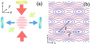
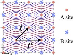
Figure 1. (a) Scheme of single mode cavity with interacting Bose gases. The pumping field is in the z direction, and the cavity field is in the x direction. (b) Emergent lattice configuration on xz plane in a superradiant cavity. t is along the diagonal $\overline{{xz}}$ direction and $t^{\prime} $ is along the x direction. |
The optical lattice VL(r) + VC(r) has a typical potential contour in the xz plane as shown in figure 1 (b). We project the motion of the atoms to the lowest band of VL(r) + VC(r), and obtain a tight-binding model
$\begin{eqnarray}\begin{array}{rcl}H & = & -t\sum _{\langle {\boldsymbol{ij}}{\rangle }_{\overline{{xz}}}}({\hat{b}}_{{\boldsymbol{i}}}^{\dagger }{\hat{b}}_{{\boldsymbol{j}}}^{}+h.c.)-{t}_{y}\sum _{\langle {\boldsymbol{i}}{\boldsymbol{j}}{\rangle }_{y}}({\hat{b}}_{{\boldsymbol{i}}}^{\dagger }{\hat{b}}_{{\boldsymbol{j}}}^{}+h.c.)\\ & & -t^{\prime} \sum _{\langle \langle {\boldsymbol{ij}}\rangle {\rangle }_{x}}({\hat{b}}_{{\boldsymbol{i}}}^{\dagger }{\hat{b}}_{{\boldsymbol{j}}}^{}+h.c.)+{H}_{\mathrm{MI}}-{\delta }_{c}| \alpha {| }^{2},\end{array}\end{eqnarray}$
$\begin{eqnarray}{H}_{\mathrm{MI}}=\displaystyle \frac{U}{2}\sum _{{\boldsymbol{i}}}{\hat{n}}_{{\boldsymbol{i}}}({\hat{n}}_{{\boldsymbol{i}}}-1)-{\mu }_{\alpha }\sum _{{\boldsymbol{i}}}{\hat{n}}_{{\boldsymbol{i}}},\end{eqnarray}$
where the field operator bi annihilates a boson on site i [ = (ix, iy, iz)(π/k0)]. Here ⟨ij⟩ and ⟨⟨ij⟩⟩ denote the nearest neighbor (NN) and the next nearest neighbor (NNN) respectively; the additional subindices x, y and $\overline{{xz}}$ restrict the neighboring sites along these specific directions. The parameters t and ty are the NN hopping strength in the xz plane and along the y-direction respectively, and $t^{\prime} $ is the NNN hopping strength along the x-direction. The chemical potential μα = μ − η(α + α*) −V0∣α∣2 includes the onsite energy shift due to the cavity field and U is the onsite interaction strength.1(1see supplementary material for details.) The total lattice site number is NΛ.2.2. Effective field theory derivation: a new method dealing with degenerate perturbation
To study phase transitions in the presence of the cavity field α, we proceed to derive from equation (1 ) an effective field theory involving α and the low energy degrees of freedom of the bosons.
To begin, we introduce a local superfluid order parameter φ ≡ W⟨bi⟩ where $W=4t+2t^{\prime} +2{t}_{y}$. We note that due to the long range coherence, the superfluid phase φ is site-independent. Assuming we are in the vicinity of SF-to-MI transition where superfluid order is weak, we can obtain an effective mean field theory of φ perturbatively from equation (1 ) as follows [21]. We first diagonalize the on-site Hamiltonian ${H}_{\mathrm{MI}}=\tfrac{U}{2}{\sum }_{{\boldsymbol{i}}}{n}_{{\boldsymbol{i}}}({n}_{{\boldsymbol{i}}}-1)-{\mu }_{\alpha }{\sum }_{{\boldsymbol{i}}}{n}_{{\boldsymbol{i}}}$ to obtain the Mott eigenstates ∣ℓ⟩, where ℓis the atomic site occupation number. Then, by approximating the tunneling part in equation (1 ) at the mean field level by ${b}_{{\boldsymbol{i}}}^{\dagger }{b}_{{\boldsymbol{j}}}^{}=({\varphi }^{* }{b}_{{\boldsymbol{j}}}^{}+{b}_{{\boldsymbol{i}}}^{\dagger }\varphi )/W-| \varphi {| }^{2}/{W}^{2}$, we calculate the energy correction to the Mott eigenstates due to such a tunneling term.
Here we focus on the energetically degenerate point of two adjacent Mott insulator phases with occupation numbers ℓand ℓ + 1. At such a point, εℓ = εℓ+1 leading to μα = νℓ = Uℓ, where ${\epsilon }_{{\ell }}\equiv \langle {\ell }| {\hat{H}}_{\mathrm{MI}}| {\ell }\rangle /{N}_{{\rm{\Lambda }}}$. To obtain accurate results around μα ≈ νℓ, we follow three steps. First, we carry out the non-degenerate perturbation in the subspace of {∣ℓ⟩, ∣ℓ − 1⟩, ∣ℓ − 2⟩} and {∣ℓ + 1⟩, ∣ℓ + 2⟩, ∣ℓ + 3⟩} to find two ‘restricted ground states' ∣L⟩ and ∣H⟩ in each subspace. The ground state ∣L⟩ can be calculated as,
$\begin{eqnarray}\begin{array}{rcl}| L\rangle \, & = & \,{{ \mathcal N }}_{L}\,\left(| {\ell }\rangle -\left(\displaystyle \frac{\sqrt{{\ell }}{\varphi }^{* }}{{\epsilon }_{{\ell }-1}-{\epsilon }_{{\ell }}}-\displaystyle \frac{\sqrt{{{\ell }}^{3}}| \varphi {| }^{2}{\varphi }^{* }}{{\left({\epsilon }_{{\ell }-1}-{\epsilon }_{{\ell }}\right)}^{3}}\right.\right.\\ & & \left.+\displaystyle \frac{\sqrt{{\ell }}({\ell }-1)| \varphi {| }^{2}{\varphi }^{* }}{{\left({\epsilon }_{{\ell }-1}-{\epsilon }_{{\ell }}\right)}^{2}({\epsilon }_{{\ell }-2}-{\epsilon }_{{\ell }})}\right)| {\ell }-1\rangle \\ & & \left.+\displaystyle \frac{\sqrt{{\ell }({\ell }-1)}{\left({\varphi }^{* }\right)}^{2}}{({\epsilon }_{{\ell }-1}-{\epsilon }_{{\ell }})({\epsilon }_{{\ell }-2}-{\epsilon }_{{\ell }})}| {\ell }-2\rangle \right),\end{array}\end{eqnarray}$
where εj = − (μ + η(α + α*))j + Uj(j − 1)/2. Similarly, the second dressed ground state ∣H⟩ in subspace {∣ℓ + 1⟩, ∣ℓ + 2⟩, ∣ℓ + 3⟩} can be obtained as $\begin{eqnarray}\begin{array}{rcl}| H\rangle \, & = & \,{{ \mathcal N }}_{H}\,\left(| {\ell }+1\rangle \,-\,\displaystyle \frac{\sqrt{{\ell }+2}\varphi }{{\epsilon }_{{\ell }+2}-{\epsilon }_{{\ell }+1}}\,\left(1-\displaystyle \frac{({\ell }+2)| \varphi {| }^{2}}{{\left({\epsilon }_{{\ell }+2}-{\epsilon }_{{\ell }+1}\right)}^{2}}\right.\right.\\ & & \left.+\displaystyle \frac{({\ell }+3)| \varphi {| }^{2}}{{\left({\epsilon }_{{\ell }+3}-{\epsilon }_{{\ell }+1}\right)}^{2}}\right)\,| {\ell }+2\rangle \,\\ & & \left.+\,\displaystyle \frac{\sqrt{({\ell }+2)({\ell }+3)}{\left(\varphi \right)}^{2}}{({\epsilon }_{{\ell }+2}\,-\,{\epsilon }_{{\ell }+\,1})({\epsilon }_{{\ell }+3}\,-\,{\epsilon }_{{\ell }+\,1})}| {\ell }\,+\,3\rangle \right),\end{array}\end{eqnarray}$
where ${{ \mathcal N }}_{L}$ and ${{ \mathcal N }}_{H}$ are normalization factors.In the second step, we write down the reduced hamiltonian in the Hilbert space spanned by ∣L⟩ and ∣H⟩, which is
$\begin{eqnarray}\begin{array}{l}{\hat{h}}_{\mathrm{red}}=\displaystyle \frac{1}{{N}_{{\rm{\Lambda }}}}\,\left(\begin{array}{cc}\langle L| {{ \mathcal H }}_{\mathrm{MF}}| L\rangle & \langle L| {{ \mathcal H }}_{\mathrm{MF}}| R\rangle \\ \langle R| {{ \mathcal H }}_{\mathrm{MF}}| L\rangle & \langle R| {{ \mathcal H }}_{\mathrm{MF}}| R\rangle \end{array}\right)\\ \,=\,-\displaystyle \frac{{\delta }_{c}}{{N}_{{\rm{\Lambda }}}}| \alpha {| }^{2}+\displaystyle \frac{| \varphi {| }^{2}}{W}\\ +\,\left(\begin{array}{cc}{\epsilon }_{{\ell }}-{\chi }_{L}| \varphi {| }^{2}+{u}_{L}| \varphi {| }^{4} & {{ \mathcal N }}_{L}{{ \mathcal N }}_{R}\sqrt{{\ell }+1}{\varphi }^{* }\\ {{ \mathcal N }}_{L}{{ \mathcal N }}_{R}\sqrt{{\ell }+1}\varphi & {\epsilon }_{{\ell }+1}-{\chi }_{R}| \varphi {| }^{2}+{u}_{R}| \varphi {| }^{4}\end{array}\right),\end{array}\end{eqnarray}$
where χL = ℓ/(εℓ−1 − εℓ), χR = (ℓ + 2)/(εℓ+2 − εℓ+1), $\begin{eqnarray}{u}_{L}=\displaystyle \frac{{{\ell }}^{2}}{{\left({\epsilon }_{{\ell }-1}-{\epsilon }_{{\ell }}\right)}^{3}}-\displaystyle \frac{{\ell }({\ell }-1)}{{\left({\epsilon }_{{\ell }-1}-{\epsilon }_{{\ell }}\right)}^{2}({\epsilon }_{{\ell }-2}-{\epsilon }_{{\ell }})},\end{eqnarray}$
$\begin{eqnarray}{u}_{R}=\displaystyle \frac{{\left({\ell }+2\right)}^{2}}{{\left({\epsilon }_{{\ell }+2}-{\epsilon }_{{\ell }+1}\right)}^{3}}-\displaystyle \frac{({\ell }+2)({\ell }+3)}{{\left({\epsilon }_{{\ell }+2}-{\epsilon }_{{\ell }+1}\right)}^{2}({\epsilon }_{{\ell }+3}-{\epsilon }_{{\ell }+1})}.\end{eqnarray}$
The smaller eigenvalue of ${\hat{h}}_{\mathrm{red}}$ is the ground state energy density, which can be obtained as $\begin{eqnarray}\begin{array}{l}{ \mathcal E }=-\displaystyle \frac{{\delta }_{c}}{{N}_{{\rm{\Lambda }}}}| \alpha {| }^{2}+\displaystyle \frac{{\epsilon }_{{\ell }}+{\epsilon }_{{\ell }+1}}{2}+r| \varphi {| }^{2}+u| \varphi {| }^{4}\\ -\,\sqrt{{{ \mathcal N }}_{L}^{2}{{ \mathcal N }}_{R}^{2}({\ell }+1)| \varphi {| }^{2}+,{\left(\displaystyle \frac{{\epsilon }_{{\ell }+1}-{\epsilon }_{{\ell }}}{2}-\bar{\chi }| \varphi {| }^{2}+\bar{u}| \varphi {| }^{4}\right)}^{2}},\end{array}\end{eqnarray}$
where ${{ \mathcal N }}_{L}^{2}{{ \mathcal N }}_{R}^{2}=1-{\ell }| \varphi {| }^{2}/{\left({\epsilon }_{{\ell }-1}-{\epsilon }_{{\ell }}\right)}^{2}$ $-({\ell }+2)| \varphi {| }^{2}/{\left({\epsilon }_{{\ell }+2}-{\epsilon }_{{\ell }+1}\right)}^{2}$, r = 1/W − (χL + χR)/2, $\bar{\chi }=({\chi }_{R}-{\chi }_{L})/2$, u = (uL + uR)/2 and $\bar{u}=({u}_{R}-{u}_{L})/2$.In a simplified way, we drop the explicit ∣φ∣4 order,
$\begin{eqnarray}\begin{array}{rcl}{ \mathcal E } & = & \,-\displaystyle \frac{{\delta }_{c}}{{N}_{{\rm{\Lambda }}}}| \alpha {| }^{2}+({\epsilon }_{{\ell }}+{\epsilon }_{{\ell }+1})/2+r| \varphi {| }^{2}\\ & & \,-\sqrt{{\left(({\epsilon }_{{\ell }+1}-{\epsilon }_{{\ell }})/2-\bar{\chi }| \varphi {| }^{2}\right)}^{2}+({\ell }+1)| \varphi {| }^{2}}.\end{array}\end{eqnarray}$
Finally, we insert in equation (9 ) the steady state solution of cavity field α determined by ${\rm{i}}{\partial }_{t}\alpha =\partial \langle \hat{H}\rangle /\partial {\alpha }^{* }-{\rm{i}}\kappa \alpha =0$. The most important assumption here is that the atomic gases reach a thermal equilibrium state when the cavity field reaches a steady state. This approximation is more valid when the decay rate κ is much larger than the atomic recoil energy ${E}_{r}\,\equiv {k}_{0}^{2}/2m$, which means the atoms' motion follows the cavity field motion almost adiabatically. Here m is the mass of the atom, the latter equation gives $\alpha =\eta {N}_{{\rm{\Lambda }}}\langle \hat{n}\rangle /({\delta }_{c}+{\rm{i}}\kappa )$. Here $\langle \hat{n}\rangle $ is the average occupation number per site. In solving for α, we have used the fact that ${U}_{0}{N}_{{\rm{\Lambda }}}\langle \hat{n}\rangle /{\delta }_{c}\ll 1$ and neglected the higher order terms In this approximation, self-consistent steady state solutions and energy density minimum are identical to each other.
An important point in our treatment is that we have eliminated the cavity strength α in favor of the occupation number ⟨n⟩ by means of the steady state equation. As we will discover later, energy degeneracy between two Mott insulating phases could result in an extra approximate symmetry by flipping the sign of $\langle \hat{n}\rangle -{\ell }-\tfrac{1}{2}$, therefore it is better to introduce a density order11 ) are relegated to (see Ref 21). Equation (11 ) is the effective theory for our following analysis of the superradiant Mott transition.
$\begin{eqnarray}\theta \equiv \langle \hat{n}\rangle -\left({\ell }+\displaystyle \frac{1}{2}\right),\end{eqnarray}$
to reveal this hidden symmetry. Then by replacing α with θ, we get the energy density as a function of density order θ and superfluid order φ in the following form $\begin{eqnarray}\begin{array}{rcl}{ \mathcal E } & = & {{ \mathcal E }}_{c}{\theta }^{2}+r| \varphi {| }^{2}\\ & & -\sqrt{({\ell }+1)| \varphi {| }^{2}+{\left({{ \mathcal E }}_{c}\theta +U\delta +\bar{\chi }| \varphi {| }^{2}\right)}^{2}}+{ \mathcal O }({\varphi }^{4}),\end{array}\end{eqnarray}$
where ${{ \mathcal E }}_{c}\equiv -{\delta }_{c}N{\eta }^{2}/({\delta }_{c}^{2}+{\kappa }^{2})\gt 0$, and $\delta =(\mu +2{{ \mathcal E }}_{c}({\ell }\,+1/2)-U{\ell })/2U;$ the detuning δ quantifies the deviation from the degenerate point μα = νℓ. Note that r and $\bar{\chi }$ are implicit functions of θ, and $\bar{\chi }\sim 0$ as θ ∼ 0. Details of the derivation equation (3. A liquid–gas-like transition between superfluids
3.1. Phase transition prediction based on effective field theory
In the limit of large pumping field strengths, the optical lattice potential is deep and the hopping strengths are small such that r is positive and large. As a result the energy density ${ \mathcal E }$ is minimized at φ = 0 for any θ, namely the system is in the Mott insulator phase. In this case we have
$\begin{eqnarray}{ \mathcal E }={{ \mathcal E }}_{c}{\theta }^{2}-| {{ \mathcal E }}_{c}\theta +U\delta | .\end{eqnarray}$
As expected, ${ \mathcal E }$ is further minimized at θ = 1/2 (⟨n⟩ = ℓ + 1) for positive detuning δ and at θ = −1/2 (⟨n⟩ = ℓ) for negative δ. Right at δ = 0, ${ \mathcal E }$ is symmetric under the transformation θ → −θ. One could find the total symmetry of the low energy theory is $U(1)\times {{\mathbb{Z}}}_{2}$ at δ = 0, which enlarges the exact symmetry of the original hamiltonian. A nonzero δ breaks the ${{\mathbb{Z}}}_{2}$ symmetry explicitly and its sign change drives a first order transition between two Mott insulators.To include a more general case for φ ≠ 0, we introduce ${{ \mathcal E }}_{c}{\rm{\Theta }}\equiv {{ \mathcal E }}_{c}\theta +U\delta +\bar{\chi }| \varphi {| }^{2}$. Then the square root term in equation (11 ) becomes $\sqrt{({\ell }+1)| \varphi {| }^{2}+{\left({{ \mathcal E }}_{c}{\rm{\Theta }}\right)}^{2}}$. To get an expansion of this term, there are two possible situations, one is Θ being finite, φ → 0, another is φ being finite and Θ → 0. The first case could be satisfied when Θ reflection symmetry is explicitly broken, that is, large δ case. In this limit we carry out a Taylor expansion in terms of φ in equation (11 ) and get
$\begin{eqnarray}\begin{array}{l}{ \mathcal E }={{ \mathcal E }}_{c}{\theta }^{2}-| {{ \mathcal E }}_{c}\theta +U\delta | \\ \quad +\left(r-\displaystyle \frac{1}{2}\displaystyle \frac{({\ell }+1)+2({{ \mathcal E }}_{c}\theta +U\delta )\bar{\chi }}{| {{ \mathcal E }}_{c}\theta +U\delta | }\right)| \varphi {| }^{2}+{u}_{4}| \varphi {| }^{4},\end{array}\end{eqnarray}$
where the u4∣φ∣4 term with u4 > 0 is added phenomenologically. For large and negative Uδ, the minimum of ${ \mathcal E }$ is located on the θ > 0 side. An SF-to-MI transition is triggered when $r-({\ell }+1)/2({{ \mathcal E }}_{c}\theta +U\delta )-\bar{\chi }$ changes sign. On the other hand, for large and positive δ, the minimum ${ \mathcal E }$ is located at θ < 0 side, where an SF-to-MI transition occurs when $r\,+({\ell }+1)/2({{ \mathcal E }}_{c}\theta +U\delta )+\bar{\chi }$ changes sign. These two transitions are traditional second order Landau–Ginzberg transitions between supefluid and Mott insulator. The boundaries of the transitions are shown as black lines in figure 2.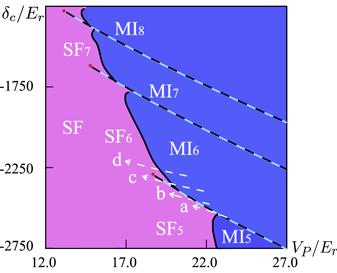
Figure 2. Phase diagram of Mott transition in superradiance phase. SF phase is in red while MI phases are in blue. Black lines represent second order transitions and the blue black dashed lines represent first order transitions. ‘liquid–vapour' critical point is marked in the red dot. White dashed lines are the paths for δ = 0, 0.005, 0.011 and 0.0125. MIℓ labels Mott insulator phase with density ℓ, SFℓ labels superfluid phase with approximate density ℓ. |
In the second case we require ${{ \mathcal E }}_{c}{\rm{\Theta }}\ll | \varphi | $, which is satisfied as long as the theory has approximate ‘θ reflection symmetry' (Θ → −Θ), namely $U\delta +\bar{\chi }| \varphi {| }^{2}=0$. This is a high ${{\mathbb{Z}}}_{2}$ symmetric region. In this region we can carry out a Taylor expansion of Θ in equation (11 ) and get
$\begin{eqnarray}\begin{array}{rcl}{ \mathcal E } & = & {{ \mathcal E }}_{0}\,-\,2\left(U\delta \,+\,\bar{\chi }| \varphi {| }^{2}\right){\rm{\Theta }}\\ & & \,+\,\left({{ \mathcal E }}_{c}\,-\,\displaystyle \frac{{{ \mathcal E }}_{c}^{2}}{2\sqrt{{\ell }\,+\,1}| \varphi | }\right){{\rm{\Theta }}}^{2}+\displaystyle \frac{{{ \mathcal E }}_{c}^{4}}{4\sqrt{{\left({\ell }\,+\,1\right)}^{3}}| \varphi {| }^{3}}{{\rm{\Theta }}}^{4},\end{array}\end{eqnarray}$
where ${{ \mathcal E }}_{0}=r| \varphi {| }^{2}\,-\,\sqrt{{\ell }\,+\,1}| \varphi | \,-\,\tfrac{{\left(U\delta \,+\,\bar{\chi }| \varphi {| }^{2}\right)}^{2}}{{{ \mathcal E }}_{c}}\,+\,{u}_{4}| \varphi {| }^{4}$. At a fine-tuned point where the linear term in the above expression disappears and the ‘θ reflection symmetry' is restored, a second order transition is triggered by ${{ \mathcal E }}_{c}\,-{{ \mathcal E }}_{c}^{2}/\sqrt{{\ell }+1}| \varphi | \leqslant 0$. In this scenario, the symmetry is spontaneously broken, leading to either a positive Θ for ‘liquid' superfluid with high density and a negative Θ for the ‘gas' superfluid with low density. A first order transition between two SFs could be engendered by the sign change of the linear Θ term, in analogy with the addition of an external magnetic field in a ferromagnet. A first order transition between a high density Mott insulator to low density superfluid is also possible as a continuation of liquid–vapour-like transition between two SFs. The existence of the liquid–vapour-like transition is the consequence of the emergent ${{\mathbb{Z}}}_{2}$ ‘θ reflection symmetry' being broken.3.2. Numerical mean field solution
Additional numerical simulation can be carried out based on our effective field theory up to ∣φ∣4 order. The phase diagram is shown in figure 2 where black and the black blue dashed lines represent the boundaries of the second order and the first order transitions, respectively; the red points represent the critical points. Four routes a, b, c and d for small δ around ‘θ reflection symmetric' region are taken across these boundaries and the order parameters along them are shown in figure 3. Along route a, δ = 0, a second order SF-to-MI transition is triggered by lowering the puming strength. For δ = 0 and large pumping strength, the system is on the θ reflection symmetric line where two Mott insulators are degenerate. Along route b, a first order transition between the Mott insulator and superfluid is displayed by a jump of the order parameter in both φ and $\langle \hat{n}\rangle $. Along route c, there are two transitions. From right to left, the first one is a second order SF-to-MI transition by a spontaneous breaking of the U(1) symmetry in φ; the second one is the liquid–vapour-like transition between two SFs. Finally, along path d, there is only a second order MI-to-SF transition. But there is an obvious kink in both superfluid order and density order at pumping strength VP = 18.75Er as we labeled by vertical dashed line in figure 3(d).
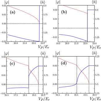
Figure 3. In (a), (b), (c), (d), the order parameters φ(dashed red) and ⟨n⟩(solid blue) along paths δ = 0, 0.005, 0.011 and 0.0125 (labeled as a, b , c, d in figure 2 as white dashed lines) are given. We use black dashed lines to label phase transition points. In (a), the SF-to-MI transition happens when φ becomes nonzero; in (b), a first order transition is labeled; in (c), there are two transitions; in (d), the right side dashed line is an SF-to-MI transition and the left side dashed line labels the kink. |
Here we identify the kink in the derivative of density order against pumping strength ${\partial }_{{V}_{P}}\langle n\rangle $. We find a critical scaling law as $| {V}_{P}-{V}_{P}^{\mathrm{cr}}{| }^{-1}$ for the maximal ${\partial }_{{V}_{P}}\langle n\rangle $, which is divergent at critical point. Here ${V}_{P}^{\mathrm{cr}}$ is the pumping strength for the critical point. This criticality is shown in figures 4 (a) and (b). To understand this criticality, we compare ${\partial }_{\delta }\langle \hat{n}\rangle $ to magnetic susceptibility. In equation (14 ), we can observe Θ plays the role of magnetization m and δ plays the role of external magnetic field h, therefore ∂δ⟨n⟩ ∝ ∂δΘ is similar to ∂hm. For Ising ferromagnetic transition, Curie–Weiss law gives ∂hm ∝ 1/∣T − Tc∣ where Tc is critical temperature. By this comparison, we know $| {V}_{P}-{V}_{P}^{\mathrm{cr}}{| }^{-1}$ scaling law of the kink is a reflection of the universal critical exponent γ for compressibility. At the same time, as the density difference θ is the order parameter, we can also measure the order parameter critical exponent β by measuring superradiance field strength.
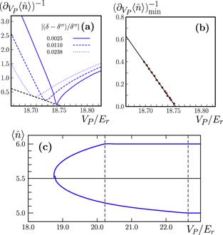
Figure 4. (a) ${\left({\partial }_{{V}_{P}}\langle \hat{n}\rangle \right)}^{-1}$ as a function of pumping field strength VP for different δ. δcr is the imbalance δ at critical point. (b) The minimal of ${\left({\partial }_{{V}_{P}}\langle \hat{n}\rangle \right)}^{-1}$ for different δ as a function of VP. The correlation coefficient of linear scaling is 0.9997. (c) In this figure, we fix δ to sit on the liquid–vapour transition point at each pumping strength VP. On the two sides of the ‘liquid–vapour transition' line, the density order is different. Here we label both density order parameters on each side of the transition point. If the density order is an integer, it is in MI phase and if the density order is not an integer, it is in superfluid phase. We observe three regions along the transition line, when VP/Er > 23, the density difference between two phases is 1, this is MI-to-MI transition; when 20.2 < VP/Er < 23, it is MI-to-SF transition; when 18.75 < VP/Er < 20.2, the transition is between two SFs. |
Concerning experimental observation, the negative kink is more difficult to observe for technical reasons. As is shown by the white dashed line d in figure 2 for fixed δ, the route we take always bypasses the critical point from above, where only positive kinks are accessed. This is consistent with the experimental procedure where similar routes are taken.
4. Conclusion and outlook
To conclude, we construct an effective field theory from a microscopic model to study the Mott transition in emergent lattices and find a liquid–vapour-like transition between two superfluids. The liquid–vapour-like transition ends at a critical point within the superfluid phase, and a divergent density kink is predicted. This kink exists in a large region around the critical point and the maximal density slope scales as $| {V}_{P}-{V}_{P}^{\mathrm{cr}}{| }^{-1}$. We link the critical exponent extracted in the kink slope with the compressibility critical exponent γ, and this could be tested by leaking photon counting measurement in an experiment. Because the present liquid–vapour-like transition is driven by quantum fluctuations and the nature of this transition is non-equilibrium, the experimental discovery of critical exponent γ will not only include the mean field result but also show corrections from quantum fluctuations and the non-equilibrium effect. By quantum fluctuation effects, we mean those effects due to spatial quantum fluctuations in the quantum critical region, which we expect to have a difference in thermal fluctuations. By the non-equilibrium effect, we mean those effects from the atomic gas distribution deviation from the thermal equilibrium state. The situation is more severe when the cavity decay rate is comparable to the recoil energy, in which case the equilibrium is hard to establish. These studies will enrich studies for first order transitions in the quantum region.
Appendix. Tight-binding model parameters
In this section, we present the construction of a tight-binding model from an emergent lattice. Assuming the condensed cavity field strength is $\alpha =\langle \hat{a}\rangle =\mathrm{Re}(\alpha )+\mathrm{iIm}(\alpha )$. $\mathrm{Re}(\alpha )$ and $\mathrm{Im}(\alpha )$ are real and imaginary part α. Then the potential for the atomic gas can be characterized as
$\begin{eqnarray}\begin{array}{l}{V}_{\mathrm{op}}({\boldsymbol{r}})=-{V}_{P}{\cos }^{2}({k}_{0}z)+{V}_{y}{\cos }^{2}({k}_{0}y)\\ \,+\,\eta (\alpha +{\alpha }^{* })\cos ({k}_{0}x)\cos ({k}_{0}z)+{V}_{0}| \alpha {| }^{2}{\cos }^{2}({k}_{0}x),\end{array}\end{eqnarray}$
where k0 is the wave number. Here VP, Vy and V0∣α∣2 are lattice strength along $\hat{z}$-direction, $\hat{y}$-direction and $\hat{x}$-direction, respectively. $\eta =-\sqrt{-{V}_{P}{V}_{0}}$ is the interaction strength between atoms and the cavity field.The possible local minima of the lattice potential Vop(r) are at rsite = (π/k0)(m, l, n)($m,l,n\in {\mathbb{Z}}$), satisfying ${\left.{\partial }_{{\boldsymbol{r}}}{V}_{\mathrm{op}}({\boldsymbol{r}})\right|}_{{\boldsymbol{r}}={{\boldsymbol{r}}}_{\mathrm{site}}}=0$. For a fixed l, the lattices are in $\hat{x}\hat{z}$-plane. The saddle points in $\hat{x}\hat{z}$-plane are shown as red dots and blue crosses in figure 5. When the cavity detune δc is much larger than the cavity decay rate κ, one can find that only A sites are local minima and B sites are saddle points.
Figure 5. Illustration of optical lattice configuration. The contour plot shows the equal potential energy lines. From red to blue, the potential becomes deeper. A sites are which are local minima of the lattice potential. B sites are saddle points of the lattice potential. t and $t^{\prime} $ are nearest and next-to-nearest hoppings between two A sites. |
In the tight-binding limit, we can only consider the nearest and next-to-nearest hoppings between two A sites. Here we denote the nearest hopping strength as t, and denote the next-to-nearest hopping strength as $t^{\prime} $. t and $t^{\prime} $ are shown in figure 5. At the same time, we can define ty as the nearest hopping between site (m, l, n) and site (m, l ± 1, n). ty can be get by WKB approximation as
$\begin{eqnarray}{t}_{y}/{E}_{r}=| {V}_{y}/{E}_{r}{| }^{3/4}{{\rm{e}}}^{-2\sqrt{| {V}_{y}/{E}_{r}| }},\end{eqnarray}$
where ${E}_{r}={k}_{0}^{2}/2m$ is the recoil energy. In a similar way, the hopping strength t and $t^{\prime} $ can be obtained as $\begin{eqnarray}t/{E}_{r}={\left|{V}_{{xx}}/2{E}_{r}\right|}^{3/4}{{\rm{e}}}^{-2\sqrt{| {V}_{{xx}}/{E}_{r}| }},\end{eqnarray}$
$\begin{eqnarray}t^{\prime} /{E}_{r}={\left|{V}_{2x}/{E}_{r}\right|}^{3/4}{{\rm{e}}}^{-2\sqrt{| {V}_{2x}/{E}_{r}| }(\sqrt{1+v}+\mathrm{Arcsinh}(v)/v)},\end{eqnarray}$
where ${V}_{{xx}}=-{V}_{P}+2\eta \mathrm{Re}(\alpha )+{V}_{0}{\alpha }^{* }\alpha $, V2x = η(α + α*) and v = 2V0∣α∣2/η(α + α*).On the other hand, the onsite interaction energy can be given in terms of the Wannier wave function Φ(r) withA5 ), the on-site interaction energy can be calculated as1 ) in the main text.
$\begin{eqnarray}U=g\int {{\rm{d}}}^{3}{\boldsymbol{r}}{{\rm{\Phi }}}^{4}({\boldsymbol{r}}).\end{eqnarray}$
The Wannier wave function Φ(r) can be approximated as ∏i=x,y,zφ(xi), where $\phi ({x}_{i})={\left({\omega }_{i}/\pi {\hslash }\right)}^{1/4}{{\rm{e}}}^{-{\omega }_{i}{x}_{i}^{2}/2{\hslash }}$ (i = x, y, z). Here ωi is the harmonic trap frequency of the local optical lattice potential in i-direction (i = x, y, z). According to equation ( $\begin{eqnarray}U=\bar{U}\sqrt{{\omega }_{x}{\omega }_{z}/{E}_{r}^{2}},\end{eqnarray}$
where ωy's dependence has been absorbed in $\bar{U}$. In terms of t, $t^{\prime} $, ty and U, we can then construct the tight-binding model equation (