


1. Introduction
Dimensionality plays a fundamental role in determining the properties of quantum many-body systems. It underpins many remarkable phenomena such as the high-Tc superconductivity [1] and magic-angle graphene [2–4] in two dimensions (2D) and the Tomonaga–Luttinger liquid [5] in 1D. Therefore, there are ongoing interests and great efforts in investigating how dimensionality affects the properties of quantum many-body systems.
Tightly confined Bose–Einstein condensate (BEC) [6] provides an ideal playground for the theoretical and experimental explorations of the dimensional effects. In particular, the state-of-the-art technology allows the depth of an optical lattice to be arbitrarily tuned by changing the laser intensities, enabling realizations of quasi-1D [7] and quasi-2D [8, 9] BECs. Thus, an important direction of investigation consists of studying the properties of a BEC system in the dimensional crossover.
Along this research line, considerable research has been carried out. For instance, [10, 11] have shown that the presence of a 2D lattice can induce a 3D to 1D crossover in the behavior of quantum fluctuations; [12–14] have investigated quantum phases along the 3D–2D crossover and the visualization of the dimensional effects in collective excitations. These works [10–13, 15, 16, 14, 17] consider the tight confinement scheme that gives rise to a direct dimensional crossover from 3D to 2D or 1D (i.e. 3D–2D or 3D–1D crossover). Instead, we will be interested in the hierarchical dimensional crossovers, i.e. the 3D-quasi-2D-1D dimensional crossovers.
We will be interested in the effect of dimensionality on not only the ground state energy and quantum depletion but also the transport properties. This is motivated by experimental realizations of BECs in the presence of disorder [18, 19]. For example, superfluidity represents a kinetic property of a system, and the superfluid density is a transport coefficient determined by the linear response theory. In this work, we investigate the 3D-quasi-2D-1D crossovers in the properties of a disorder BEC trapped in an anisotropic optical lattice, using the Green function approach. Specifically, we calculate the ground-state energy and quantum depletion, as well as the superfluid density, and we analyze the combined effects of dimensionality and disorder.
2. Model
At zero temperature, an optically-trapped BEC can be well described by the N-body Hamiltonian [10–13]1 ), Vopt(r) and Vran(r), respectively, describe the anisotropic 2D optical lattice and the external random potential.
$\begin{eqnarray}\begin{array}{rcl}\hat{H}-\mu \hat{N} & = & \int {\rm{d}}{\boldsymbol{r}}{\hat{{\rm{\Psi }}}}^{\dagger }({\boldsymbol{r}})\left[-\displaystyle \frac{{{\hslash }}^{2}{{\rm{\nabla }}}^{2}}{2m}-\mu +{V}_{\mathrm{opt}}({\boldsymbol{r}})+{V}_{\mathrm{ran}}({\boldsymbol{r}})\right.\\ & & \left.+\displaystyle \frac{{g}}{2}{\hat{{\rm{\Psi }}}}^{\dagger }\hat{{\rm{\Psi }}}\right]\hat{{\rm{\Psi }}}({\boldsymbol{r}}),\end{array}\end{eqnarray}$
where $\hat{{\rm{\Psi }}}({\boldsymbol{r}})$ is the field operator for bosons with mass m, μ is the chemical potential, $\hat{N}=\int {\rm{d}}{\boldsymbol{r}}{\hat{{\rm{\Psi }}}}^{\dagger }({\boldsymbol{r}}){\rm{\Psi }}({\boldsymbol{r}})$ is the number operator, and g = 4πℏ2a3D /m is the coupling constant with a3D being the 3D scattering length [20]. In Hamiltonian (We consider the anisotropic 2D optical lattice in Hamiltonian (1 ) in the form [6]
$\begin{eqnarray}{V}_{\mathrm{opt}}({\boldsymbol{r}})={E}_{R}\left[{V}_{1}{\sin }^{2}({q}_{B}x)+{V}_{2}{\sin }^{2}({q}_{B}y)\right],\end{eqnarray}$
where V1,2 denote the laser intensities and ${E}_{R}={{\hslash }}^{2}{q}_{B}^{2}/2m$ is the recoil energy, with ℏqB being the Bragg momentum and m the atomic mass. The lattice period is fixed by d = π/qB. Atoms are free in the z direction. By controlling the depths of the optical lattice V1 and V2, crossovers to low dimensions are expected to occur via the hierarchical access of new energy scales: firstly, a 3D Bose gas becomes quasi-2D when the energetic restriction to freeze x-direction excitations is reached; next, by further freezing the kinetic energy along the y-direction, the quasi-2D BEC is expected to enter the quasi-1D regime.Moreover, in Hamiltonian (1 ), ${V}_{\mathrm{ran}}({\boldsymbol{r}})={\sum }_{i}^{{N}_{\mathrm{imp}}}v({\boldsymbol{r}}-{{\boldsymbol{r}}}_{i})$ can be produced by the random potential [21, 11, 13]. For sufficiently dilute disorder [18, 19], v(r) can be approximated by an effective pseudopotential, i.e. v(r) = gimpδ(r), where ${g}_{\mathrm{imp}}=2\pi {{\hslash }}^{2}\tilde{b}/m$ is the effective coupling constant of an impurity-boson pair and $\tilde{b}$ is the effective scattering length accounting for the presence of a 2D optical lattice [22, 23].
We assume the lattice depths V1 and V2 in equation (2 ) in the unit of the recoil energy of ER are relatively large (V1 ≥ 5, V2 ≥ 5), so that the interband gap of Egap is bigger than the chemical potential of μ, i. e. Egap ≫ μ. Meanwhile, because of the quantum tunneling, the overlap of the wave functions of two consecutive wells is still sufficient to ensure full coherence even in the presence of disorder. By this assumption [10–13], we restrict ourselves to the lowest band, where the physics is governed by the ratio between the chemical potential μ and the bandwidth of 4(J1 + J2), where J1 and J2 are the tunneling rates between neighboring wells. Generally speaking, for 4(J1 + J2) ≫ μ, the system retains an anisotropic 3D behavior, whereas for 4(J1 + J2) ≃ μ, the system undergoes a dimensional crossover to a 1D regime. In the limit of 4(J1 + J2) ≪ μ, the model system can be treated as 1D. Following [10–13], we treat our model system within the tight-binding approximation as shown in appendix A . The lowest Bloch band of the model system can be described in terms of the Wannier functions as ${\phi }_{{k}_{x}}(x){\phi }_{{k}_{y}}(y)$, with ${\phi }_{{k}_{{x}_{i}}}({x}_{i})={\sum }_{l}{{\rm{e}}}^{{\rm{i}}{{ldk}}_{{x}_{i}}}w({x}_{i}-{ld})$. Here, $w({x}_{i})=\exp \left[-{x}_{i}^{2}/2{\sigma }_{i}^{2}\right]/{\pi }^{1/4}{\sigma }_{i}^{1/2}$ and $d/{\sigma }_{i}=\pi {V}_{i}^{1/4}\exp \left(-1/4\sqrt{{V}_{i}}\right)$ (i = 1, 2 and x1 = x, x2 = y). We remark that this work is limited to a tight-binding approximation by neglecting beyond-lowest-Bloch-band transverse modes along the x and y directions. Further considering the effects of beyond-lowest-Bloch-band transverse modes on the dimensional crossover goes beyond the scope of this work.
Directly following [11, 13], we expand the field operators in Hamiltonian (1 ) as $\hat{{\rm{\Psi }}}({\boldsymbol{r}})={\sum }_{{\boldsymbol{k}}}{\hat{a}}_{{\boldsymbol{k}}}{{\rm{e}}}^{-{\rm{i}}{k}_{z}z}{\phi }_{{k}_{x}}(x){\phi }_{{k}_{y}}(y)$ and obtain3 ) is the Fourier transform of disorder potential.
$\begin{eqnarray}\begin{array}{rcl}H-\mu N & = & \sum _{{\boldsymbol{k}}}\left({\varepsilon }_{{\boldsymbol{k}}}^{0}-\mu \right){\hat{a}}_{{\boldsymbol{k}}}^{\dagger }{\hat{a}}_{{\boldsymbol{k}}}+\displaystyle \frac{\tilde{g}}{2V}\sum _{{\boldsymbol{k}},{\boldsymbol{q}},{{\boldsymbol{k}}}^{{\prime} }}{\hat{a}}_{{\boldsymbol{k}}+{\boldsymbol{q}}}^{\dagger }{\hat{a}}_{{{\boldsymbol{k}}}^{{\prime} }-{\boldsymbol{q}}}^{\dagger }{\hat{a}}_{{{\boldsymbol{k}}}^{{\prime} }}{\hat{a}}_{{\boldsymbol{k}}}\\ & & +\sum _{{\boldsymbol{k}},{{\boldsymbol{k}}}^{{\prime} }}{\hat{a}}_{{\boldsymbol{k}}}^{\dagger }{\hat{a}}_{{{\boldsymbol{k}}}^{{\prime} }}{V}_{{\boldsymbol{k}}-{{\boldsymbol{k}}}^{{\prime} }},\end{array}\end{eqnarray}$
where $\begin{eqnarray}{\varepsilon }_{{\boldsymbol{k}}}^{0}=\displaystyle \frac{{{\hslash }}^{2}{k}_{z}^{2}}{2m}+2\left[J-{J}_{1}\cos {k}_{x}-{J}_{2}\cos {k}_{y}\right],\end{eqnarray}$
is the energy dispersion of the non-interacting system. Here, J1 and J2 are the tunneling rates along the x- and y-direction, respectively. Moreover, we have J = J1 + J2, V is the volume of the model system, and $\tilde{g}={{g}{\rm{d}}}^{2}/(2\pi {\sigma }_{1}{\sigma }_{2})$ is the renormalized coupling constant. The Vk = 1/V∫eik·rVrandr in equation (We remark that in this work, we do not consider the effect of the confinement-induced resonance (CIR) [24, 25] on the coupling constant $\tilde{g}$. The basic physics of CIR can be understood in the language of Feshbach resonance [26], where the scattering open channel and closed channels are, respectively, represented by the ground-state transverse mode and the other transverse modes along the tight-confinement dimensions. Within the tight-binding approximation assumed in this work, the ultracold atoms are frozen in the states of the lowest Bloch band and can not be excited into the other transverse modes. Thus the effect of CIR on $\tilde{g}$ can be safely ignored as the closed channels are absent [24–26].
Our subsequent calculations proceed in two steps. First, we calculate the ground state energy and quantum depletion. Previous studies [11, 13] have shown that the effects of disorder simply lead to trivial energy shifts in the ground state energy, and therefore, we shall ignore the disorder potential in this part of calculations and set Vran = 0. Second, we investigate how the dimensionality affects the superfluid density in the presence of the disorder potential Vran ≠ 0.
3. Ground state energy and quantum depletion
For an optically-trapped Bose gas described by Hamiltonian (1 ), the ground state energy Eg and quantum depletion can be calculated via the single-particle Green function G(k, ω) [27] as follows5 ) and (6 ), the G(k, ω) is the Fourier transformation of the Green function
$\begin{eqnarray}\displaystyle \frac{{E}_{g}}{V}\,=\,\displaystyle \frac{\tilde{g}{n}^{2}}{2}\,+\,\mathop{\mathrm{lim}}\limits_{t\to 0-}\,\displaystyle \frac{1}{{\left(2\pi \right)}^{3}{{\rm{d}}}^{2}}\,\int \,{\rm{d}}{k}_{z}{{\rm{d}}}^{2}{\boldsymbol{k}}\,\int \,\displaystyle \frac{{\rm{d}}\omega }{2\pi {\rm{i}}}{{\rm{e}}}^{-{\rm{i}}\omega t}\,{E}_{{\boldsymbol{k}}}G({\boldsymbol{k}},\omega ),\end{eqnarray}$
$\begin{eqnarray}\displaystyle \frac{N-{N}_{0}}{N}\,=\,\mathop{\mathrm{lim}}\limits_{t\to 0-}\displaystyle \frac{{\rm{i}}}{{\left(2\pi \right)}^{4}{{d}}^{2}n}\int {\rm{d}}{k}_{z}{{\rm{d}}}^{2}{\boldsymbol{k}}\int {\rm{d}}\omega {{\rm{e}}}^{-{\rm{i}}\omega t}G({\boldsymbol{k}},\omega ),\end{eqnarray}$
with E(k) being the excitation energy. In equations ( $\begin{eqnarray}G({\boldsymbol{k}},t-{t}^{{\prime} })=-{\rm{i}}\left\langle T{\hat{a}}_{{\boldsymbol{k}}}(t){\hat{a}}_{{\boldsymbol{k}}}^{\dagger }({t}^{{\prime} })\right\rangle ,\end{eqnarray}$
in the Heisenberg representation, where T denotes the chronological product.By applying the Bogoliubov theory [10–14] to the Hamiltonian (1 ), we follow the standard procedures and obtain4 ).
$\begin{eqnarray}G({\boldsymbol{k}},\omega )=\displaystyle \frac{\omega +{\varepsilon }_{{\boldsymbol{k}}}^{0}+\tilde{g}n}{{\omega }^{2}-{E}_{{\boldsymbol{k}}}^{2}+{\rm{i}}0}.\end{eqnarray}$
Here, n0 is the condensate density, ${E}_{{\boldsymbol{k}}}=\sqrt{{\varepsilon }_{{\boldsymbol{k}}}^{0}({\varepsilon }_{{\boldsymbol{k}}}^{0}+2\tilde{g}n)}$ and ${\varepsilon }_{{\boldsymbol{k}}}^{0}$ is defined in equation (By plugging equation (8 ) into equations (5 ) and (6 ), respectively, the ground state energy Eg and quantum depletion (N − N0)/N are straightforwardly obtained (see the detailed derivations in appendix B )9 ) and (10 ), the functions f(s) and h(s), respectively, are given by11 ) and (12 ), the variable s stands for $s={s}_{1}\,+{s}_{2}=2({J}_{1}+{J}_{2})/\tilde{g}n$, which can be controlled by the strength of optical lattice in equation (2 ), and $\gamma =1-({J}_{1}/J)\cos {k}_{x}\,-({J}_{2}/J)\cos {k}_{y}$. The function ${}_{2}{F}_{1}\left(a,b,c,d\right)$ in equation (11 ) is the hypergeometric function.
$\begin{eqnarray}\displaystyle \frac{{E}_{g}}{V}=\displaystyle \frac{1}{2}\tilde{g}{n}^{2}-\displaystyle \frac{\sqrt{2m\tilde{g}n}\tilde{g}n}{4\pi {\hslash }{d}^{2}}f\left(\displaystyle \frac{2J}{\tilde{g}n}\right),\end{eqnarray}$
and $\begin{eqnarray}\displaystyle \frac{N-{N}_{0}}{N}=\displaystyle \frac{1}{4\pi {\hslash }{d}^{2}}\sqrt{\displaystyle \frac{2m\tilde{g}}{n}}h\left(\displaystyle \frac{2J}{\tilde{g}n}\right).\end{eqnarray}$
In equations ( $\begin{eqnarray}f(s)=\displaystyle \frac{\pi }{2}{\int }_{-\pi }^{\pi }\displaystyle \frac{{{\rm{d}}}^{2}{\boldsymbol{k}}}{{\left(2\pi \right)}^{2}}\displaystyle \frac{1}{\sqrt{s\gamma }}{}_{2}{F}_{1}\left[\displaystyle \frac{1}{2},\displaystyle \frac{3}{2},3,\displaystyle \frac{-2}{s\gamma }\right],\end{eqnarray}$
and $\begin{eqnarray}\begin{array}{l}h(s)={\int }_{-\pi }^{\pi }\displaystyle \frac{{{\rm{d}}}^{2}{\boldsymbol{k}}}{{\left(2\pi \right)}^{2}}{\int }_{0}^{\infty }\displaystyle \frac{{\rm{d}}\eta }{\sqrt{\eta }}\\ \,\times \,\left[\displaystyle \frac{\eta +s\gamma +1}{\sqrt{\left(\eta +s\gamma \right)\left(\eta +s\gamma +2\right)}}-1\right].\end{array}\end{eqnarray}$
In equations (Equations (9 ) and (10 ) are the key results of this work. In figures 1 and 2, we plot f(s) and h(s), respectively. In the limit s → ∞ , the system is anisotropic 3D, whereas in the opposite limit s → 0, the system is 1D. Thus, when continuously decreasing $s=2({J}_{1}+{J}_{2})/\tilde{g}n$ by enhancing the confinement, the system necessarily crossovers from the anisotropic 3D to 1D.We emphasize that the 3D-like gas here is referred as to an optically-trapped Bose gas in the tight-binding approximation, which is different from 3D Bose gas in the almost free space. However, from the theoretical angles, we can extend the parameter regimes from tight-binding-3D-gas to beyond-tight-binding-3D-gas, i.e. entering the parameter regime of V1 < 5, V2 < 5. In what follows, we are surprised to find that our analytical results can recover the Lee–Huang–Yang results obtained from the 3D free space as a surprising bonus of our analytical results. To induce the hierarchical dimensional crossover, we consider the following scheme for controlling the lattice depths, which consists of two stages: (i) we first fix the lattice strength V1 = 5 and increase V2 from the initial strength of V2 = 5 to the final strength of V2 = 12 (i.e. s2 is decreased to almost zero), where the system is expected to crossover from the 3D to the quasi-2D; (ii) we fix V2 = 12 and further increase the value of V1 from the initial strength of V1 = 5 to the final strength of V1 = 12 until the value of s = s1 + s2 is almost zero.
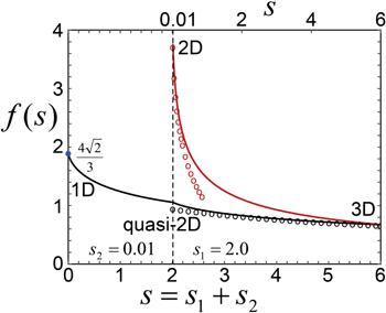
Figure 1. Scaling function f(s) in equation ( |
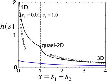
Figure 2. The behavior of h(s) as the dimensionless tunneling rates of s1,2 change independently. In the left side of the vertical dashed line, we fix s2 = 0.01 and set s1 = [0, 1]. In the right side, we fix s1 = 1 and set s2 = [0.01, 3]. The BEC behaves from 1D-like to quasi-2D like, and finally to 3D-like, as s increases. The two black dotted lines denote the 1D and 3D asymptotic behaviors respectively. The blue curve describes the disorder-induced quantum depletion along the dimensional crossover, which is plotted by the functions $\tfrac{{g}_{\mathrm{imp}}^{2}{n}_{\mathrm{imp}}}{4\pi {\tilde{g}}^{2}n}{\int }_{-\pi }^{\pi }{{\rm{d}}}^{2}{\boldsymbol{k}}{\left(2+s\gamma \right)}^{-\tfrac{3}{2}}$ with ${g}_{\mathrm{imp}}^{2}{n}_{\mathrm{imp}}/({\tilde{g}}^{2}n)=0.1$. |
In process (i), the behavior of the functions of f(s) and h(s) are shown by the solid curves in figures 1 and 2. Let us first check whether our analytical results in equations (9 ) and (10 ) in the limit s → ∞ can recover the well-known 3D results of Bose gases. For s → ∞ , corresponding to the anisotropic 3D regime, we find $f(s)\simeq 1.43\sqrt{2/s}-32\sqrt{2}/(15\pi s)$ in equation (11 ) and $h(s)\simeq 8/(3\pi \sqrt{2}s)$, as denoted by the black circled curves in figures 1 and 2, respectively. Thus we exactly recover the 3D results of the quantum ground state energy and quantum depletion in [13]. We note that our work is different from [13], where one adds a 1D optical lattice and increases the lattice depth to realize a purely 2D system. Instead, our scheme realizes the quasi-2D quantum system. To compare the two, we also plot the f(s) associated with the case in [13] [see red curves in figure 1]. As clearly shown, our scheme realizes a quasi-2D (black curve), instead of a purely 2D, quantum system before it further crossovers to quasi-1D.
In process (ii), we increase V1 and fix the lattice depth V2, where the system is expected to crossover from the quasi-2D to the quasi-1D and then to pure 1D. In particular, we note that the function f(s) shown in figure 1 exactly approaches $3\sqrt{2}/4$ in the limit s → 0, corresponding to the Lieb–Liniger result of 1D Bose gas in [10]. For the quantum depletion shown in figure 2, the function h(s) diverges as $h(s)\simeq -\mathrm{ln}(1.35s)/\sqrt{2}$. This signals that in the absence of tunneling there is no real BEC, in agreement with the general theorems in one dimension.
4. Superfluid density
In the second part of this paper, we apply the linear response theory to investigate the effects of disorder on the superfluid density of the BEC trapped in a 2D optical lattice. The superfluid density ρs is determined by the response of the momentum density to an externally imposed velocity field. We calculate ρs based on the Bogoliubov approximation. Note that [21] pioneered in the study of the superfluid density of a 3D disordered Bose gas within the framework of Bogoliubov theory, which is consistent with the results obtained by the Beliaev–Popov diagrammatic technique [28]. In the context of ultracold Bose gas, one of the authors in [11, 13] has investigated the disorder-induced superfluid density along the 3D–1D dimensional crossover using the Bogoliubov approximation.
In a disordered BEC, the static current-current response function consists of the low-frequency, long-wavelength longitudinal response ${\chi }_{L}\left({\boldsymbol{k}}\right)$ and the transverse response ${\chi }_{T}\left({\boldsymbol{k}}\right)$, i.e. ${\chi }_{{ij}}\left({\boldsymbol{k}}\right)=\tfrac{{k}_{i}{k}_{j}}{{k}^{2}}{\chi }_{L}\left({\boldsymbol{k}}\right)+({\delta }_{{ij}}-\tfrac{{k}_{i}{k}_{j}}{{k}^{2}}){\chi }_{T}\left({\boldsymbol{k}}\right)$, see details of the definition of χij in [11, 13]. The transverse response of a BEC is only due to the normal fluid, since the superfluid component can only participate in the irrotational flow.
For the disordered BEC trapped in a 2D optical lattice described by Hamiltonian (1 ), where the rotational symmetry is broken, the response function along the unconfined z direction is different from that in the confined x–y plane. In the following, we assume a slow rotation with respect to the z axis and calculate the transverse response function along the z direction. We find13 ) can be interpreted as the second-order term in the perturbation expansion of the normal-fluid density in terms of the weak disorder Vk.
$\begin{eqnarray}\begin{array}{rcl}{\rho }_{n} & = & \mathop{\mathrm{lim}}\limits_{k\to 0}{\chi }_{T}\left({\boldsymbol{k}}\right)={\chi }_{{zz}}(0,0)=\displaystyle \frac{2n}{m}\sum _{p}\displaystyle \frac{{p}_{z}^{2}{\varepsilon }_{{\boldsymbol{k}}}^{0}}{{E}^{4}({\boldsymbol{k}})}\langle | {V}_{{\boldsymbol{k}}}{| }^{2}\rangle \\ & = & \displaystyle \frac{\tilde{R}\sqrt{2m\tilde{g}n}}{16{\hslash }{d}^{2}}I(s),\end{array}\end{eqnarray}$
where $\tilde{R}={n}_{\mathrm{imp}}{\tilde{b}}^{2}/n{\tilde{a}}_{3D}^{2}$ and I(s) with $s={s}_{1}+{s}_{2}\,=2({J}_{1}+{J}_{2})/\tilde{g}n$ is given by $\begin{eqnarray}I(s)={\int }_{-\pi }^{\pi }\displaystyle \frac{{{\rm{d}}}^{2}{\boldsymbol{k}}}{{\left(2\pi \right)}^{2}}\displaystyle \frac{2}{\sqrt{s\gamma +2}(s\gamma +1+\sqrt{s\gamma (s\gamma +2)})}.\end{eqnarray}$
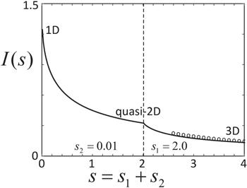
Equation (The result of equation (13 ) is plotted in figure 3. In the asymptotic 3D limit, one finds $I(s)\simeq 4\sqrt{2}/(3\pi s)$, corresponding to the dotted curve in figure 3. In this case, equation (13 ) recovers the corresponding result of 3D Bose gases as in [13]. Equation (13 ) presents another key result of this paper, which provides an analytical expression for the normal fluid density in a Bose fluid in an anisotropic two-dimensional optical lattice with the presence of weak disorder. The superfluid density ρs = ρ − ρn is thus straightforwardly obtained.
Figure 3. The behavior of I(s) as the dimensionless tunneling rates of s1,2 change independently. On the left side of the vertical dashed line, we fix s2 = 0.01 and set s1 = [0, 2]. In the right side, we fix s1 = 2 and set s2 = [0.01, 2]. The BEC behaves from 1D-like to quasi-2D-like, and finally to 3D-like, as s increases. The black dotted line on the right side denotes the 3D asymptotic behavior. |
5. Discussion and conclusion
We justify the Bogoliubov approximation used in our calculations a posteriori by estimating the quantum depletion [10]. The experimental work [29] by Ketterle's group has shown that the Bogoliubov theory provides a semiquantitative description for an optically-trapped BEC even when the quantum depletions are in excess of 50%. For a uniform BEC, the quantum depletion is $(N-{N}_{0})/N=8/3\sqrt{{{na}}_{3D}^{2}}$ and the Bogoliubov approximation is valid provided $\sqrt{{{na}}_{3D}^{2}}$ is small. For an optically-trapped BEC, the quantum depletion is modified qualitatively as $(8{m}^{* }/3m)\sqrt{n{\tilde{a}}_{3D}/\pi }$ with m* being the effective mass, which remains small for typical experimental parameters as in [10]. For an optically-trapped Bose gas along the dimensional crossovers, we can estimate the quantum depletion (N − N0)/N with the help of figure 2. Considering typical experiments in an optically-trapped BEC as in [6], the relevant parameters are n = 3 × 1013 cm−3, d = 430 nm, a3D = 5.4 nm, and d/σ1 ∼ d/σ2 ∼ 1. The quantum depletion in equation (10 ) is thus evaluated as (N − N0)/N ∼ 0.0036 × h(s), with h(s) shown in figure 2. It is clear that the quantum depletion (N − N0)/N < 20%, and therefore, the Bogoliubov approximation is valid in the spirit of [29]. Apart from the phase fluctuations due to the tight confinement along x and y-directions, the effect of the disorder potential can also enhance quantum fluctuations and thus affect the Bogoliubov approximation. As such, we calculate the disorder-induced correction to the quantum depletion as
$\begin{eqnarray}\displaystyle \frac{{\rm{\Delta }}{N}^{{\prime} }}{N}=\displaystyle \frac{1}{4\pi {\hslash }{d}^{2}}\sqrt{\displaystyle \frac{2m\tilde{g}}{n}}\displaystyle \frac{{g}_{\mathrm{imp}}^{2}{n}_{\mathrm{imp}}}{4\pi {\tilde{g}}^{2}n}{\int }_{-\pi }^{\pi }{{\rm{d}}}^{2}{\boldsymbol{k}}{\left(2+s\gamma \right)}^{-\tfrac{3}{2}}.\end{eqnarray}$
For the case of weak disorder of ${g}_{\mathrm{imp}}^{2}{n}_{\mathrm{imp}}/{\tilde{g}}^{2}n=0.1$ with nimp being the impurity density, the quantum depletion due to the disorder along the dimensional crossover is shown by the blue curves in figure 2. This result indicates the quantum depletion due to the disorder is small and the Bogoliubov approximation is still valid.In summary, we have investigated a 3D disordered BEC trapped in an anisotropic 2D optical lattice characterized by the lattice depths of V1 in the x-direction and V2 in the y-direction, respectively. We have derived the analytical expressions of the ground-state energy, quantum depletion and superfluid density of the system. Our results show the hierarchical, 3D-quasi-2D-1D crossovers in the behavior of quantum fluctuations and the superfluid density. The physics of the hierarchical dimensional crossover involves the interplay of three quantities: the strength of the optical lattice, the interaction between bosonic atoms, and the strength of disorder. All these quantities are experimentally controllable using state-of-the-art technologies. In particular, the depth of an optical lattice can be tuned from 0ER to 32ER almost at will [6]. Therefore, the phenomena discussed in this paper should be observable within the current experimental capabilities. Observing this hierarchical dimensional effect directly would present an important step in revealing the interplay between dimensionality and quantum fluctuations in quasi-low dimensions. The present work is based on the Bogoliubov theory. Future studies in this direction include the treatment of the system for the whole range of interatomic interaction strength, from zero to infinity, as well as for arbitrarily strong disorder.
Note added
Before submitting our work, we notice that a similar work [17] has studied the 2D–1D dimensional crossover. In contrast, our work has focused on the gradual 3D–2D–1D dimensional crossover.
Appendix A. Validity of tight-binding approximation
In the tight-binding approximation [6], the tunnelling rates of J1 and J2 along the x- and y-directions are defined as2 ) are relatively large (V1 ≥ 5, V2 ≥ 5) to make sure that the interband gap of Egap is bigger than the chemical potential of μ, i. e. Egap ≫ μ; (ii) the overlap of the wave functions of two consecutive wells are still sufficient to ensure full coherence because of the quantum tunneling.
$\begin{eqnarray}{J}_{1}={\int }_{-\infty }^{\infty }{\rm{d}}{{xw}}^{* }(x)\left(-\displaystyle \frac{{{\hslash }}^{2}}{2m}\displaystyle \frac{{\partial }^{2}}{\partial {x}^{2}}+{V}_{1}\times {E}_{R}{\sin }^{2}({q}_{B}x)\right)w(x),\end{eqnarray}$
$\begin{eqnarray}{J}_{2}={\int }_{-\infty }^{\infty }{\rm{d}}{{yw}}^{\ast }(y)\left(-\displaystyle \frac{{\hslash }^{2}}{2m}\displaystyle \frac{{{\rm{\partial }}}^{2}}{{\rm{\partial }}{y}^{2}}+{V}_{2}\times {E}_{R}{\sin }^{2}({q}_{B}y)\right)w(y),\end{eqnarray}$
with w(x) and w(y) being the Wannier functions in the x- and y-directions. The analytic solutions for the Wannier functions can be obtained by solving the 1D Mathieu problem as shown in [30]. In such, the approximate analytic expressions of tunnelling rates J1 and J2 have been derived in [31] $\begin{eqnarray}\displaystyle \frac{{J}_{1}}{{E}_{R}}=\displaystyle \frac{1}{4}{\left(\displaystyle \frac{2}{\pi }\right)}^{\tfrac{1}{2}}{\left(\displaystyle \frac{{V}_{1}}{4}\right)}^{\tfrac{3}{4}}{2}^{5}\exp \left(-2\sqrt{{V}_{1}}\right),\end{eqnarray}$
$\begin{eqnarray}\displaystyle \frac{{J}_{2}}{{E}_{R}}=\displaystyle \frac{1}{4}{\left(\displaystyle \frac{2}{\pi }\right)}^{\tfrac{1}{2}}{\left(\displaystyle \frac{{V}_{2}}{4}\right)}^{\tfrac{3}{4}}{2}^{5}\exp \left(-2\sqrt{{V}_{2}}\right).\end{eqnarray}$
In order for analytical expressions of J1 and J2 to be valid, the considered energy band must be a slowly varying function of the quasi-momentum. Hence, the potential depth s must be sufficiently large. Note that the tight-binding approximation is valid under the following conditions (i) lattice depths od V1 and V2 in equation (Now we are ready to give the rough estimations of parameter regimes of the tight-binding approximation being valid. Here, we use the typically experimental parameters of an optically-trapped Bose gas in [32]. The typical detailed parameters read as follows: the recoil energy is ER ≈ h × 3.33 kHz with h being Plank constant and the chemical potential of gas is $\mu \approx \tilde{g}n\approx h\times 400\,\mathrm{Hz}$. In the case of (V1 ≈ 5, V2 ≈ 5), we can estimate the parameters of J1/ER ≈ J2/ER ≈ 0.09 based on equations (A3 ) and (A4 ). Then we can further estimate the dimensionless parameters used in the figures of this work as follows: $s=2({J}_{1}+{J}_{2})/\tilde{g}n=(2({J}_{1}+{J}_{2})/{R}_{R})$ $({E}_{R}/\tilde{g}n)\,\approx 2\,\times \,$(0.09 + 0.09) × 10 = 3.6, suggesting that our model system is 3D-like. Meanwhile, as shown in [32], the optically-trapped Bose gas is entirely superfluid below the critical lattice height Vc ≈ 13ER corresponding to J1 and J2 being almost zero because of the exponential decrease in equations (A3 ) and (A4 ). We conclude that the tight-binding approximation can be regarded to be valid under 5 < V1 < 13 and 5 < V2 < 13, corresponding to 0 < s < 4 as shown in figures 1 and 2.
Appendix B. Detailed derivations of equations (9 ) and (10 )
In this appendix, we give the detailed derivations of equations (9 ) and (10 ). The derivation of equation (9 ) in the main text can be written as follows9 ) in the main text10 ) in the main text is as follows
$\begin{eqnarray}\begin{array}{rcl}\displaystyle \frac{{E}_{g}}{V} & = & \displaystyle \frac{\tilde{g}{n}^{2}}{2}+\mathop{\mathrm{lim}}\limits_{t\to 0-}\displaystyle \frac{1}{{\left(2\pi \right)}^{3}{{d}}^{2}}\int {\rm{d}}{k}_{z}{{\rm{d}}}^{2}{\boldsymbol{k}}\int \displaystyle \frac{{\rm{d}}\omega }{2\pi {\rm{i}}}{{\rm{e}}}^{-{\rm{i}}\omega t}{E}_{{\boldsymbol{k}}}G({\boldsymbol{k}},\omega )\\ & = & \displaystyle \frac{\tilde{g}{n}^{2}}{2}+\displaystyle \frac{1}{{\left(2\pi \right)}^{3}{{d}}^{2}}\int {\rm{d}}{k}_{z}{{\rm{d}}}^{2}{\boldsymbol{k}}{\int }_{C}\displaystyle \frac{{\rm{d}}\omega }{2\pi {\rm{i}}}{E}_{{\boldsymbol{k}}}G({\boldsymbol{k}},\omega ),\end{array}\end{eqnarray}$
with $\begin{eqnarray}\begin{array}{rcl}{\int }_{C}{\rm{d}}\omega G({\boldsymbol{k}},\omega ) & = & {\int }_{C}{\rm{d}}\omega \displaystyle \frac{\omega +{\varepsilon }_{{\boldsymbol{k}}}^{0}+\tilde{g}n}{{\omega }^{2}-{E}_{{\boldsymbol{k}}}^{2}+{\rm{i}}0}\\ & = & {\int }_{C}{\rm{d}}\omega \displaystyle \frac{\omega +{\varepsilon }_{{\boldsymbol{k}}}^{0}+\tilde{g}n}{2{E}_{{\boldsymbol{k}}}}\\ & & \times \,\left(\displaystyle \frac{1}{\omega -{E}_{{\boldsymbol{k}}}+{\rm{i}}0}-\displaystyle \frac{1}{\omega +{E}_{{\boldsymbol{k}}}-{\rm{i}}0}\right)\\ & = & 2\pi {\rm{i}}\mathop{\mathrm{lim}}\limits_{\omega \to -{E}_{{\boldsymbol{k}}}+{\rm{i}}0}\displaystyle \frac{\omega +{\varepsilon }_{{\boldsymbol{k}}}^{0}+\tilde{g}n}{2{E}_{{\boldsymbol{k}}}}\\ & & \times \,\left(\omega +{E}_{{\boldsymbol{k}}}-{\rm{i}}0\right)\displaystyle \frac{-1}{\omega +{E}_{{\boldsymbol{k}}}-{\rm{i}}0}\\ & = & -\pi {\rm{i}}\displaystyle \frac{{\varepsilon }_{{\boldsymbol{k}}}^{0}+\tilde{g}n-{E}_{{\boldsymbol{k}}}}{{E}_{{\boldsymbol{k}}}},\end{array}\end{eqnarray}$
where we have used the residue theorem, and C denotes the integration path around the upper half-plane. Then we have $\begin{eqnarray}\begin{array}{rcl}\displaystyle \frac{{E}_{g}}{V} & = & \displaystyle \frac{\tilde{g}{n}^{2}}{2}-\displaystyle \frac{1}{{\left(2\pi \right)}^{3}{{d}}^{2}2}{\int }_{-\pi }^{\pi }{{\rm{d}}}^{2}{\boldsymbol{k}}{\int }_{-\infty }^{\infty }{\rm{d}}{k}_{z}\left({\varepsilon }_{{\boldsymbol{k}}}^{0}+\tilde{g}n-{E}_{{\boldsymbol{k}}}\right)\\ & = & \displaystyle \frac{\tilde{g}{n}^{2}}{2}-\mathrm{Int},\end{array}\end{eqnarray}$
with $\begin{eqnarray}\begin{array}{rcl}\mathrm{Int} & = & \displaystyle \frac{1}{{\left(2\pi \right)}^{3}{{d}}^{2}2}{\int }_{-\pi }^{\pi }{{\rm{d}}}^{2}{\boldsymbol{k}}{\int }_{-\infty }^{\infty }{\rm{d}}{k}_{z}({\varepsilon }_{{\boldsymbol{k}}}^{0}+\tilde{g}n-{E}_{{\boldsymbol{k}}})\\ & = & \displaystyle \frac{1}{{\left(2\pi \right)}^{3}{{d}}^{2}2}{\int }_{-\pi }^{\pi }{{\rm{d}}}^{2}{\boldsymbol{k}}{\int }_{-\infty }^{\infty }{\rm{d}}{k}_{z}\left(\displaystyle \frac{{{\hslash }}^{2}{k}_{z}^{2}}{2m}+2J\gamma +\tilde{g}n\right.\\ & & \left.-\sqrt{\left(\displaystyle \frac{{{\hslash }}^{2}{k}_{z}^{2}}{2m}+2J\gamma \right)\left(\displaystyle \frac{{{\hslash }}^{2}{k}_{z}^{2}}{2m}+2J\gamma +2\tilde{g}n\right)}\right)\\ & = & \displaystyle \frac{1}{{\left(2\pi \right)}^{3}{{d}}^{2}2{\hslash }}{\int }_{-\pi }^{\pi }{{\rm{d}}}^{2}{\boldsymbol{k}}{\int }_{-\infty }^{\infty }{\rm{d}}{p}_{z}\left(\displaystyle \frac{{p}_{z}^{2}}{2m}+2J\gamma +\tilde{g}n\right.\\ & & \left.-\sqrt{\left(\displaystyle \frac{{p}_{z}^{2}}{2m}+2J\gamma \right)\left(\displaystyle \frac{{p}_{z}^{2}}{2m}+2J\gamma +2\tilde{g}n\right)}\right)\\ & = & \displaystyle \frac{\sqrt{2m}2}{{\left(2\pi \right)}^{3}{{d}}^{2}2{\hslash }}{\int }_{-\pi }^{\pi }{{\rm{d}}}^{2}{\boldsymbol{k}}{\int }_{0}^{\infty }{\rm{d}}{p}_{z}\left({p}_{z}^{2}+2J\gamma +\tilde{g}n\right.\\ & & \left.-\sqrt{\left({p}_{z}^{2}+2J\gamma \right)\left({p}_{z}^{2}+2J\gamma +2\tilde{g}n\right)}\right)\\ & = & \displaystyle \frac{\sqrt{2m}\tilde{g}n\sqrt{\tilde{g}n}}{{\left(2\pi \right)}^{3}{{d}}^{2}{\hslash }}{\int }_{-\pi }^{\pi }{{\rm{d}}}^{2}{\boldsymbol{k}}{\int }_{0}^{\infty }{\rm{d}}{p}_{z}\left({p}_{z}^{2}+s\gamma +1\right.\\ & & \left.-\sqrt{\left({p}_{z}^{2}+s\gamma \right)\left({p}_{z}^{2}+s\gamma +2\right)}\right),\end{array}\end{eqnarray}$
where $\gamma =1-\tfrac{{J}_{1}}{J}\cos ({k}_{x})-\tfrac{{J}_{2}}{J}\cos ({k}_{y})$ and $s=\tfrac{2J}{\tilde{g}n}$. We then let ${p}_{z}^{2}+s\gamma =\beta $, $\begin{eqnarray}\begin{array}{rcl}\mathrm{Int} & = & \displaystyle \frac{\sqrt{2m}\tilde{g}n\sqrt{\tilde{g}n}}{{\left(2\pi \right)}^{3}{{d}}^{2}{\hslash }}{\int }_{-\pi }^{\pi }{{\rm{d}}}^{2}{\boldsymbol{k}}\\ & & \times \,{\int }_{s\gamma }^{\infty }\displaystyle \frac{{\rm{d}}\beta }{2\sqrt{\beta -s\gamma }}\left(\beta +1-\sqrt{\beta \left(\beta +2\right)}\right).\end{array}\end{eqnarray}$
We then let sγ/β = τ, and dβ = −sγdτ/τ2, $\begin{eqnarray}\begin{array}{rcl}\mathrm{Int} & = & \displaystyle \frac{\sqrt{2m}\tilde{g}n\sqrt{\tilde{g}n}}{{\left(2\pi \right)}^{3}{{d}}^{2}{\hslash }2}{\int }_{-\pi }^{\pi }{{\rm{d}}}^{2}{\boldsymbol{k}}{\int }_{0}^{1}\displaystyle \frac{s\gamma }{{\tau }^{2}}{\rm{d}}\tau \displaystyle \frac{1}{\sqrt{\tfrac{s\gamma }{\tau }-s\gamma }}\\ & & \times \,\left(\displaystyle \frac{s\gamma }{\tau }+1-\sqrt{\displaystyle \frac{s\gamma }{\tau }\left(\displaystyle \frac{s\gamma }{\tau }+2\right)}\right)\\ & = & \displaystyle \frac{\sqrt{2m}\tilde{g}n\sqrt{\tilde{g}n}}{{\left(2\pi \right)}^{3}{{d}}^{2}{\hslash }2}{\int }_{-\pi }^{\pi }{{\rm{d}}}^{2}{\boldsymbol{k}}{\int }_{0}^{1}{\rm{d}}\tau \displaystyle \frac{\sqrt{s\gamma }}{\sqrt{\tau }}\displaystyle \frac{1}{\sqrt{1-\tau }}\\ & & \times \,\left(\displaystyle \frac{s\gamma }{{\tau }^{2}}+\displaystyle \frac{1}{\tau }-\displaystyle \frac{s\gamma }{{\tau }^{2}}\sqrt{1+\displaystyle \frac{2\tau }{s\gamma }}\right)\\ & = & \displaystyle \frac{\sqrt{2m}\tilde{g}n\sqrt{\tilde{g}n}}{{\left(2\pi \right)}^{3}{{d}}^{2}{\hslash }2}{\int }_{-\pi }^{\pi }{{\rm{d}}}^{2}{\boldsymbol{k}}\displaystyle \frac{1}{\sqrt{s\gamma }}{\int }_{0}^{1}{\rm{d}}\tau \displaystyle \frac{1}{\sqrt{\tau }}\displaystyle \frac{1}{\sqrt{1-\tau }}\\ & & \times \,\left(\displaystyle \frac{{\left(s\gamma \right)}^{2}}{{\tau }^{2}}+\displaystyle \frac{s\gamma }{\tau }-\displaystyle \frac{{\left(s\gamma \right)}^{2}}{{\tau }^{2}}\sqrt{1+\displaystyle \frac{2\tau }{s\gamma }}\right),\end{array}\end{eqnarray}$
where the integration about τ can be written as the hypergeometric function $\begin{eqnarray}\begin{array}{l}{\int }_{0}^{1}{\rm{d}}\tau \displaystyle \frac{1}{\sqrt{\tau }}\displaystyle \frac{1}{\sqrt{1-\tau }}\left(\displaystyle \frac{{\left(s\gamma \right)}^{2}}{{\tau }^{2}}+\displaystyle \frac{s\gamma }{\tau }-\displaystyle \frac{{\left(s\gamma \right)}^{2}}{{\tau }^{2}}\sqrt{1+\displaystyle \frac{2\tau }{s\gamma }}\right)\\ =\,\displaystyle \frac{\pi }{2}{}_{2}{F}_{1}\left[\displaystyle \frac{1}{2},\displaystyle \frac{3}{2},3,\displaystyle \frac{-2}{s\gamma }\right],\end{array}\end{eqnarray}$
hence we obtain $\begin{eqnarray}\begin{array}{rcl}\mathrm{Int} & = & \displaystyle \frac{\sqrt{2m}\tilde{g}n\sqrt{\tilde{g}n}}{{\left(2\pi \right)}^{3}{{d}}^{2}{\hslash }2}{\int }_{-\pi }^{\pi }{{\rm{d}}}^{2}{\boldsymbol{k}}\displaystyle \frac{1}{\sqrt{s\gamma }}\displaystyle \frac{\pi }{2}{}_{2}{F}_{1}\left[\displaystyle \frac{1}{2},\displaystyle \frac{3}{2},3,\displaystyle \frac{-2}{s\gamma }\right]\\ & = & \displaystyle \frac{\sqrt{2m\tilde{g}n}\tilde{g}n}{4\pi {\hslash }{{d}}^{2}}\displaystyle \frac{\pi }{2}{\int }_{-\pi }^{\pi }\displaystyle \frac{{{\rm{d}}}^{2}{\boldsymbol{k}}}{{\left(2\pi \right)}^{2}}\displaystyle \frac{1}{\sqrt{s\gamma }}{}_{2}{F}_{1}\left[\displaystyle \frac{1}{2},\displaystyle \frac{3}{2},3,\displaystyle \frac{-2}{s\gamma }\right]\\ & = & \displaystyle \frac{\sqrt{2m\tilde{g}n}\tilde{g}n}{4\pi {\hslash }{{d}}^{2}}f(s),\end{array}\end{eqnarray}$
with $\begin{eqnarray}f(s)=\displaystyle \frac{\pi }{2}{\int }_{-\pi }^{\pi }\displaystyle \frac{{{\rm{d}}}^{2}{\boldsymbol{k}}}{{\left(2\pi \right)}^{2}}\displaystyle \frac{1}{\sqrt{s\gamma }}{}_{2}{F}_{1}\left[\displaystyle \frac{1}{2},\displaystyle \frac{3}{2},3,\displaystyle \frac{-2}{s\gamma }\right].\end{eqnarray}$
Finally we get the equations ( $\begin{eqnarray}\begin{array}{rcl}\displaystyle \frac{{E}_{g}}{V} & = & \displaystyle \frac{\tilde{g}{n}^{2}}{2}-\mathrm{Int}\\ & = & \displaystyle \frac{\tilde{g}{n}^{2}}{2}-\displaystyle \frac{\sqrt{2m\tilde{g}n}\tilde{g}n}{4\pi {\hslash }{d}^{2}}f(s).\end{array}\end{eqnarray}$
The derivation of equations ( $\begin{eqnarray}\begin{array}{rcl}\displaystyle \frac{N-{N}_{0}}{N} & = & \mathop{\mathrm{lim}}\limits_{t\to 0-}\displaystyle \frac{{\rm{i}}}{{\left(2\pi \right)}^{4}{{d}}^{2}n}\int {\rm{d}}{k}_{z}{{\rm{d}}}^{2}{\boldsymbol{k}}\int {\rm{d}}\omega {{\rm{e}}}^{-{\rm{i}}\omega t}G({\boldsymbol{k}},\omega )\\ & = & \displaystyle \frac{{\rm{i}}}{{\left(2\pi \right)}^{4}{{d}}^{2}n}\int {\rm{d}}{k}_{z}{{\rm{d}}}^{2}{\boldsymbol{k}}{\int }_{C}{\rm{d}}\omega G({\boldsymbol{k}},\omega )\\ & = & \displaystyle \frac{{\rm{i}}}{{\left(2\pi \right)}^{4}{{d}}^{2}n}\int {\rm{d}}{k}_{z}{{\rm{d}}}^{2}{\boldsymbol{k}}(-\pi {\rm{i}})\displaystyle \frac{{\varepsilon }_{{\boldsymbol{k}}}^{0}+\tilde{g}n-{E}_{{\boldsymbol{k}}}}{{E}_{{\boldsymbol{k}}}}\\ & = & \displaystyle \frac{1}{2{\left(2\pi \right)}^{3}{{d}}^{2}n}\int {\rm{d}}{k}_{z}{{\rm{d}}}^{2}{\boldsymbol{k}}\displaystyle \frac{{\varepsilon }_{{\boldsymbol{k}}}^{0}+\tilde{g}n-{E}_{{\boldsymbol{k}}}}{{E}_{{\boldsymbol{k}}}}\\ & = & \displaystyle \frac{1}{2{\left(2\pi \right)}^{3}{{d}}^{2}n}{\int }_{-\pi }^{\pi }{{\rm{d}}}^{2}{\boldsymbol{k}}{\int }_{-\infty }^{\infty }{\rm{d}}{k}_{z}\\ & & \times \,\left[\displaystyle \frac{\tfrac{{{\hslash }}^{2}{k}_{z}^{2}}{2m}+2J\gamma +\tilde{g}n}{\sqrt{\left(\tfrac{{{\hslash }}^{2}{k}_{z}^{2}}{2m}+2J\gamma \right)\left(\tfrac{{{\hslash }}^{2}{k}_{z}^{2}}{2m}+2J\gamma +2\tilde{g}n\right)}}-1\right]\\ & = & \displaystyle \frac{1}{2{\left(2\pi \right)}^{3}{\hslash }{{d}}^{2}n}{\int }_{-\pi }^{\pi }{{\rm{d}}}^{2}{\boldsymbol{k}}{\int }_{-\infty }^{\infty }{\rm{d}}{p}_{z}\\ & & \times \,\left[\displaystyle \frac{\tfrac{{p}_{z}^{2}}{2m}+2J\gamma +\tilde{g}n}{\sqrt{\left(\tfrac{{p}_{z}^{2}}{2m}+2J\gamma \right)\left(\tfrac{{p}_{z}^{2}}{2m}+2J\gamma +2\tilde{g}n\right)}}-1\right]\\ & = & \displaystyle \frac{\sqrt{2m}}{2{\left(2\pi \right)}^{3}{\hslash }{{d}}^{2}n}{\int }_{-\pi }^{\pi }{{\rm{d}}}^{2}{\boldsymbol{k}}{\int }_{-\infty }^{\infty }{\rm{d}}{p}_{z}\\ & & \times \,\left[\displaystyle \frac{{p}_{z}^{2}+2J\gamma +\tilde{g}n}{\sqrt{\left({p}_{z}^{2}+2J\gamma \right)\left({p}_{z}^{2}+2J\gamma +2\tilde{g}n\right)}}-1\right]\\ & = & \displaystyle \frac{\sqrt{2m}}{2{\left(2\pi \right)}^{3}{\hslash }{{d}}^{2}n}{\int }_{-\pi }^{\pi }{{\rm{d}}}^{2}{\boldsymbol{k}}\\ & & \times 2\,{\int }_{0}^{\infty }\displaystyle \frac{{\rm{d}}\eta }{2\sqrt{\eta }}\left[\displaystyle \frac{\eta +2J\gamma +\tilde{g}n}{\sqrt{\left(\eta +2J\gamma \right)\left(\eta +2J\gamma +2\tilde{g}n\right)}}-1\right]\\ & = & \displaystyle \frac{\sqrt{2m\tilde{g}n}}{2{\left(2\pi \right)}^{3}{\hslash }{{d}}^{2}n}{\int }_{-\pi }^{\pi }{{\rm{d}}}^{2}{\boldsymbol{k}}{\int }_{0}^{\infty }\displaystyle \frac{{\rm{d}}\eta }{\sqrt{\eta }}\\ & & \times \,\left[\displaystyle \frac{\eta +s\gamma +1}{\sqrt{\left(\eta +s\gamma \right)\left(\eta +s\gamma +2\right)}}-1\right]\\ & = & \displaystyle \frac{1}{4\pi {\hslash }{{d}}^{2}}\sqrt{\displaystyle \frac{2m\tilde{g}}{n}}{\int }_{-\pi }^{\pi }\displaystyle \frac{{{\rm{d}}}^{2}{\boldsymbol{k}}}{{\left(2\pi \right)}^{2}}\\ & & \times \,{\int }_{0}^{\infty }\displaystyle \frac{{\rm{d}}\eta }{\sqrt{\eta }}\left[\displaystyle \frac{\eta +s\gamma +1}{\sqrt{\left(\eta +s\gamma \right)\left(\eta +s\gamma +2\right)}}-1\right]\\ & = & \displaystyle \frac{1}{4\pi {\hslash }{{d}}^{2}}\sqrt{\displaystyle \frac{2m\tilde{g}}{n}}h(s),\end{array}\end{eqnarray}$
with $\begin{eqnarray}\begin{array}{rcl}h(s) & = & {\int }_{-\pi }^{\pi }\displaystyle \frac{{{\rm{d}}}^{2}{\boldsymbol{k}}}{{\left(2\pi \right)}^{2}}\\ & & \times \,{\int }_{0}^{\infty }\displaystyle \frac{{\rm{d}}\eta }{\sqrt{\eta }}\left[\displaystyle \frac{\eta +s\gamma +1}{\sqrt{\left(\eta +s\gamma \right)\left(\eta +s\gamma +2\right)}}-1\right].\end{array}\end{eqnarray}$