Welcome to visit Communications in Theoretical Physics,
Others

Polynomial synchronization of complex-valued inertial neural networks with multi-proportional delays

  • Zhuang Yao 1 ,
  • Ziye Zhang , 1 ,
  • Zhen Wang 1 ,
  • Chong Lin 2 ,
  • Jian Chen 3
Expand
  • 1College of Mathematics and Systems Science, Shandong University of Science and Technology, Qingdao 266590, China
  • 2Institute of Complexity Science, Qingdao University, Qingdao 266071, China
  • 3College of Automation Engineering, Qingdao University of Technology, Qingdao 266555, China

Received date: 2022-05-02

  Revised date: 2022-08-20

  Accepted date: 2022-08-23

  Online published: 2022-11-21

Copyright

© 2022 Institute of Theoretical Physics CAS, Chinese Physical Society and IOP Publishing

Abstract

This paper investigates the polynomial synchronization (PS) problem of complex-valued inertial neural networks with multi-proportional delays. It is analyzed based on the non-separation method. Firstly, an exponential transformation is applied and an appropriate controller is designed. Then, a new sufficient criterion for PS of the considered system is derived by the Lyapunov function approach and some inequalities techniques. In the end, a numerical example is given to illustrate the effectiveness of the obtained result.

Cite this article

Zhuang Yao , Ziye Zhang , Zhen Wang , Chong Lin , Jian Chen . Polynomial synchronization of complex-valued inertial neural networks with multi-proportional delays[J]. Communications in Theoretical Physics, 2022 , 74(12) : 125801 . DOI: 10.1088/1572-9494/ac8bce

1. Introduction

Neural networks (NNs) have always possessed a wide range of applications in associative memory, image processing, dynamic optimization, and machine learning [13] over the years, which have aroused many scholars' interest and produced a large number of research results [46]. In 1986, the inertial neural networks (INNs) model was produced by introducing an inductor into an artificial neural network circuit [7, 8]. Different from the artificial neural networks model described by the first-order differential equation, the INNs model obeys the second-order one and the second-order term is called the inertial term. The introduction of the inertia term can effectively improve the disordered search performance of the network, and it is also the key factor to produce complex behaviors such as bifurcation and chaos. Moreover, the inertia term itself has a strong biological background. For example, the cell membrane of some organisms can be realized by the circuit system containing inductance, and the axons of squid and penguin can be simulated by the inductance in the circuit [9]. Compared with the first-order NNs, INNs show more complex dynamic behaviors. So, it shows the extremely important theoretical significance and practical application value in studying the dynamical behaviors of INNs deeply [10, 11].
The above research results are all on the basis of real-valued neural networks with real-valued activation functions and state variables. With the involvement of complex signals, complex-valued neural networks (CVNNs) models entered the vision of scholars [1219]. It is not only a simple extension of real-valued NNs but also has the characteristics of fast calculation and strong processing ability, and it can be used to deal with some problems that cannot be solved in the real number field. Naturally, complex-valued inertial neural networks (CVINNs) have also aroused widespread concern, and the development of dynamic behavior has increased rapidly in recent years. When developing dynamic behaviors, most of the work is based on the separation method by separating the real part and imaginary part of the considered systems, such as stability analysis [2022], stabilization [23, 24], and synchronization [2529]. Later, driven by related theories in a complex number field, the non-separation method, that is, regarding the considered systems as a whole, is used fully to study various dynamics, including state estimation [30], exponential convergence [22], finite/fixed-time synchronization [28, 29, 31], anti-synchronization [23, 24, 32], and exponential and adaptive synchronization [33]. Compared with the separation method, the non-separation method can reduce conservatism and computational complexity.
Synchronization has been applied to some practical fields such as image encryption, secure communication, and brain-like intelligence, which makes it a very active research topic. Besides those synchronization issues mentioned above, there are others, for example, polynomial synchronization (PS). The concept of PS originated from polynomial stability and was first proposed in [34], which is a kind of dynamic behavior in some special cases of stochastic differential equations and wave equations [35, 36]. As stated in [37, 38], its basic characteristic is that its top Lyapunov exponent equals 0. It is called polynomial stability because its definition contains tλ(λ > 0), which is similar to the structure of polynomials. It is more general than exponential stability, which is between exponential stability and asymptotic stability. Its convergence speed is slower than that of exponential stability, but both of them can degenerate into asymptotic stability. Thus, based on these outstanding characteristics, polynomial stability is also a very typical dynamic behavior. For PS of the drive-response systems, that is, polynomial stability of the error systems, there has been no relevant result about CVINNs up to now. This fact promotes our research.
It should be pointed out that the time delay cannot be ignored in the whole design process of CVINNs. As we all know, due to the inherent delay time of inertial neurons and the limited speed of information transmission, signal acquisition, and processing between neurons, the time delay of the inertial neural system is inevitable. It is found that time delay has a great impact on the dynamic behaviors of neural networks, which may lead to instability, oscillation, and other poor performance. Therefore, it is very important to study the dynamic characteristics of delayed neural networks. As one of many delay types, the proportional delay is time-varying and unbounded with τ(t) = (1 − q)t(0 < q < 1). Due to its monotony-increasing property, the network running time can be easily controlled according to the allowable delay of the networks [39, 40]. In addition, systems with proportional delay have many interesting applications, such as nonlinear integro-differential equations, web application servers, and wireless LAN [4143]. Thus, it plays an increasingly important role in many important fields such as physics, biological systems, and control science [44, 45]. These days, there are few achievements in the dynamical behaviors of CVINNs with proportional delay [21, 31]. In [21], memristor-based CVINNs with proportional and distributed delays are studied and new results on exponential input-to-state stability by using the separation method are given. In [31], the stabilization problem for CVINNs with proportional delay is discussed via the non-separation approach and finite-time stability theory.
Considering the clear feature of multi-proportional delays [38, 46], such as more generality and reality in contrast to single-proportional delays, we will focus on the PS problem of CVINNs with multi-proportional delays in this paper. The main contributions are summarized as follows:

(1)Considering the importance of PS and proportional delay, the PS problem of CVINNs with multi-proportional delays is studied for the first time.

(2)To maintain the originality of the considered system and reduce computational pressure, our work is carried out by a non-separation approach instead of decomposition.

(3)To achieve the PS of the addressed CVINNs with multi-proportional delays, by applying the exponential transformation and designing an appropriate controller, a new criterion for PS is proposed based on the Lyapunov function approach and some inequalities techniques.

Notations: C and Cn stand for the set of complex numbers and all n-dimensional complex-valued vectors, respectively. For any zC, $| z| =\sqrt{z\overline{z}}$ denotes the module of z, where $\overline{z}$ is the conjugate of z. For any $z={\left({z}_{1},{z}_{2},\ldots ,{z}_{n}\right)}^{{\rm{T}}}\in {C}^{n}$, the norm of z is defined as $\parallel z\parallel =\sqrt{{\sum }_{j=1}^{n}| {z}_{j}{| }^{2}}$.

2. Preliminaries

In this paper, we consider the complex-valued inertial neural networks described in the following form:
$\begin{eqnarray}\begin{array}{rcl}{\ddot{u}}_{j}(t) & = & -{a}_{j}{\dot{u}}_{j}(t)-{b}_{j}{u}_{j}(t)+\displaystyle \sum _{r=1}^{n}{c}_{{jr}}{f}_{r}({u}_{r}({p}_{r}t))\\ & & +\displaystyle \sum _{r=1}^{n}{m}_{{jr}}{g}_{r}({u}_{r}({q}_{r}t))+{I}_{j}(t),\end{array}\end{eqnarray}$
where j = 1, 2,…,n, tt0 ≥ 1, uj(t) ∈ C represents the state of the jth neuron at time t; ${\ddot{u}}_{j}(t)$ indicates the inertial term; aj and bj are the positive constants; cjr and mjr are the delayed connection weight coefficients; fr(· ), gr(· ) ∈ C are complex-valued activation functions; pr, qr are proportional delays factors with pr, qr ∈ (0, 1]; prt = t − (1 − pr)t, qrt = t − (1 − qr)t, in which (1 − pr)t and (1 − qr)t are the transmission delay functions; Ij is the external input.

On one hand, as a special type of delay, the proportional delay is a time-varying and unbounded delay, which is different from constant delay, distributed delay, and so on. In many fields, such as control science, and physical and biological systems, it can be found that proportional delay plays an important role. On the other hand, as a special neural network, CVINNs have attracted extensive attention because of their rich biological and engineering background. Compared with first-order neural networks, the dynamic behaviors of the second-order CVINNs are more complex and it is more difficult to deal with them. So far, there have been few reports on CVINNs with proportional delays [21, 31]. Here, we will continue to study deeply the CVINNs model with multi-proportional delays and develop the relative achievement for the PS problem.

The initial conditions of system (1)
$\begin{eqnarray}{u}_{j}(s)={\phi }_{j}(s),{\dot{u}}_{j}(t)={\psi }_{j}(s),\end{eqnarray}$
where $s\in [\tilde{q}{t}_{0},{t}_{0}]$, $\tilde{q}={\min }_{1\leqslant r\leqslant n}\{{p}_{r},{q}_{r}\}$, φj(s) and $Psi$j(s) are continuous functions. The response system is described by
$\begin{eqnarray}\begin{array}{rcl}{\ddot{v}}_{j}(t) & = & -{a}_{j}{\dot{v}}_{j}(t)-{b}_{j}{v}_{j}(t)+\displaystyle \sum _{r=1}^{n}{c}_{{jr}}{f}_{r}({v}_{r}({p}_{r}t))\\ & & +\displaystyle \sum _{r=1}^{n}{m}_{{jr}}{g}_{r}({v}_{r}({q}_{r}t))+{I}_{j}(t)+{U}_{j}(t),\,\,\end{array}\end{eqnarray}$
where vj(t) represents the state of the response system and Uj(t) represents the control input. The initial conditions of system (3)
$\begin{eqnarray}{v}_{j}(s)=\hat{{\phi }_{j}}(s),\dot{{v}_{j}}(t)=\hat{{\psi }_{j}}(s),\end{eqnarray}$
where $s\in [\tilde{q}{t}_{0},{t}_{0}]$, $\hat{{\phi }_{j}}(s)$ and $\hat{{\psi }_{j}}(s)$ are continuous functions.
Define the synchronization error yj(t) = vj(t) − uj(t), the error system can be written as
$\begin{eqnarray}\begin{array}{rcl}{\ddot{y}}_{j}(t) & = & -{a}_{j}{\dot{y}}_{j}(t)-{b}_{j}{y}_{j}(t)+\displaystyle \sum _{r=1}^{n}{c}_{{jr}}\hat{{f}_{r}}({y}_{r}({p}_{r}t))\\ & & +\displaystyle \sum _{r=1}^{n}{m}_{{jr}}\hat{{g}_{r}}({y}_{r}({q}_{r}t))+{U}_{j}(t),\end{array}\end{eqnarray}$
where tt0, ${\hat{f}}_{r}({y}_{r}({p}_{r}t))$ = fr(vr(prt)) − fr(ur(prt)), ${\hat{g}}_{r}({y}_{r}({q}_{r}t)\,={g}_{r}({v}_{r}({q}_{r}t))-{g}_{r}({u}_{r}({q}_{r}t))$.
By introducing the following variable transformation:
$\begin{eqnarray*}{z}_{j}(t)={w}_{j}{\dot{y}}_{j}(t)+{\tilde{w}}_{j}{y}_{j}(t),\end{eqnarray*}$
where wj ≠ 0, ${\tilde{w}}_{j}$ is the appropriate constant, system (5) can be converted into
$\begin{eqnarray}\left\{\begin{array}{l}{\dot{y}}_{j}(t)=-\displaystyle \frac{{\tilde{w}}_{j}}{{w}_{j}}{y}_{j}(t)+\displaystyle \frac{1}{{w}_{j}}{z}_{j}(t),\\ {\dot{z}}_{j}(t)=-{\gamma }_{j}{z}_{j}(t)-{\zeta }_{j}{y}_{j}(t)+\displaystyle \sum _{r=1}^{n}{w}_{j}{c}_{{jr}}{\hat{f}}_{r}({y}_{r}({p}_{r}t))\\ +\displaystyle \sum _{r=1}^{n}{w}_{j}{m}_{{jr}}{\hat{g}}_{r}({y}_{r}({q}_{r}t))+{w}_{j}{U}_{j}(t),\end{array}\right.\end{eqnarray}$
where ${\gamma }_{j}={a}_{j}-\tfrac{{\tilde{w}}_{j}}{{w}_{j}}$ and ${\zeta }_{j}={b}_{j}{w}_{j}-{\gamma }_{j}{\tilde{w}}_{j}$. Let ${\hat{y}}_{j}(t)={y}_{j}({{\rm{e}}}^{t})$ and ${\hat{z}}_{j}(t)={z}_{j}({{\rm{e}}}^{t})$, we can obtain the following equivalent system for system (6)
$\begin{eqnarray}\left\{\begin{array}{l}{\hat{\dot{y}}}_{j}(t)={{\rm{e}}}^{t}\left(-\displaystyle \frac{{\tilde{w}}_{j}}{{w}_{j}}{\hat{y}}_{j}(t)+\displaystyle \frac{1}{{w}_{j}}{\hat{z}}_{j}(t)\right),\\ {\hat{\dot{z}}}_{j}(t)={{\rm{e}}}^{t}\left(-{\gamma }_{j}{\hat{z}}_{j}(t)-{\zeta }_{j}{\hat{y}}_{j}(t)+\sum _{r=1}^{n}{w}_{j}{c}_{{jr}}{\hat{f}}_{r}({\hat{y}}_{r}(t-{\mu }_{r}))\right.\\ \left.+\sum _{r=1}^{n}{w}_{j}{m}_{{jr}}{\hat{g}}_{r}({y}_{r}(t-{h}_{r}))+{w}_{j}{\tilde{U}}_{j}(t\right),\qquad t\geqslant \mathrm{log}{t}_{0},\end{array}\right.\end{eqnarray}$
with
$\begin{eqnarray}\begin{array}{rcl}{\hat{y}}_{j}(s) & = & {\xi }_{j}(s),\,{\hat{\dot{y}}}_{j}(s)={\chi }_{j}(s),\\ s & \in & [\mathrm{log}\tilde{q}{t}_{0},\mathrm{log}{t}_{0}],\end{array}\end{eqnarray}$
where ${\mu }_{r}=-\mathrm{log}{p}_{r}$, ${h}_{r}=-\mathrm{log}{q}_{r}$, ${\tilde{U}}_{j}(t)={U}_{j}({{\rm{e}}}^{t})$, ${\xi }_{j}(s)={\hat{\phi }}_{j}({{\rm{e}}}^{s})-{\phi }_{j}({{\rm{e}}}^{s})$ and ${\chi }_{j}(s)={\hat{\psi }}_{j}({{\rm{e}}}^{s})-{\psi }_{j}({{\rm{e}}}^{s})$.

In realizing the PS of the addressed model, the main difficulty and challenge are how to obtain the power exponential term ${t}^{-\lambda }$ according to the definitions of polynomial stability and synchronization. Here, firstly, the exponential transformation is involved [34]. Then, by designing a suitable controller and constructing an appropriate Lyapunov function, our purpose is achieved.

In this paper, activation functions ${f}_{r}(\cdot )$ and ${g}_{r}(\cdot )$ are assumed to satisfy the following Lipschitz conditions:

$\begin{eqnarray*}\begin{array}{rcl}| {f}_{r}(v) & & -{f}_{r}(u)| \leqslant {F}_{r}| v-u| ,\\ | {g}_{r}(v) & & -{g}_{r}(u)| \leqslant {G}_{r}| v-u| ,\,\forall v,u\in C,\end{array}\end{eqnarray*}$
where $r=1,2,\ldots ,n$, ${F}_{r}\gt 0$ and ${G}_{r}\gt 0$.

[38]. Let $v(t)={\left({v}_{1}(t),{v}_{2}(t),\ldots ,{v}_{n}(t)\right)}^{{\rm{T}}}$ and $\hat{\phi }(s)={\left({\hat{\phi }}_{1}(s),{\hat{\phi }}_{2}(s),\ldots ,{\hat{\phi }}_{n}(s)\right)}^{{\rm{T}}}$, system (1) is globally polynomially stable if there exist constants $K\geqslant 1$ and $\lambda \gt 0$ such that

$\begin{eqnarray*}\parallel v(t)-\bar{v}{\parallel }^{2}\leqslant K\parallel \hat{\phi }(s)-\bar{v}{\parallel }_{\tilde{q}}^{2}{t}^{-\lambda },\,t\geqslant {t}_{0},\end{eqnarray*}$
where $\parallel \hat{\phi }(s)-\bar{v}{\parallel }_{\tilde{q}}^{2}={\sup }_{\tilde{q}{t}_{0}\leqslant \ s\leqslant {t}_{0}}\parallel \hat{\phi }(s)-\bar{v}{\parallel }^{2}$, $\bar{v}$ is an equilibrium point of system (1).

[34]. Let $u(t)={\left({u}_{1}(t),{u}_{2}(t),\ldots ,{u}_{n}(t)\right)}^{{\rm{T}}}$ and $\phi (s)={\left({\phi }_{1}(s),{\phi }_{2}(s),\ldots ,{\phi }_{n}(s)\right)}^{{\rm{T}}}$, systems (1) and (3) can reach global polynomial synchronization if there exists constants $K\geqslant 1$ and $\lambda \gt 0$ such that

$\begin{eqnarray*}\parallel v(t)-u(t){\parallel }^{2}\leqslant K\parallel \hat{\phi }(s)-\phi (s){\parallel }_{\tilde{q}}^{2}{t}^{-\lambda },\,t\geqslant {t}_{0},\end{eqnarray*}$
where $\parallel \hat{\phi }(s)-\phi (s){\parallel }_{\tilde{q}}^{2}={\sup }_{\tilde{q}{t}_{0}\leqslant \ s\leqslant {t}_{0}}\parallel \hat{\phi }(s)-\phi (s){\parallel }^{2}$.

3. Main result

In this section, we will develop a sufficient condition to ascertain the PS for systems (1) and (3). First, we design the following control input
$\begin{eqnarray}{\tilde{U}}_{j}(t)=\left\{\begin{array}{l}-\displaystyle \frac{1}{{w}_{j}\overline{{\hat{z}}_{j}(t)}}\left({k}_{j}{\hat{y}}_{j}(t)\overline{{\hat{y}}_{j}(t)}+{\eta }_{j}{\hat{z}}_{j}(t)\overline{{\hat{z}}_{j}(t)}+\displaystyle \frac{{\rho }_{j}}{2}\sum _{r=1}^{n}{\hat{y}}_{r}(t-{\mu }_{r})\overline{{\hat{y}}_{r}(t-{\mu }_{r})}\right.\\ \left.+\displaystyle \frac{{\sigma }_{j}}{2}\sum _{r=1}^{n}{\hat{y}}_{r}(t-{h}_{r})\overline{{\hat{y}}_{r}(t-{h}_{r})}\right),\qquad \qquad \qquad \qquad | {\hat{z}}_{j}(t)| \ne 0,\\ 0,\qquad \qquad \qquad \qquad \qquad \qquad \qquad | {\hat{z}}_{j}(t)| =0,\end{array}\right.\end{eqnarray}$
where positive numbers kj, ηj, ρj and σj are control gains.

Here, the above controller (9) is designed to guarantee the PS performance for CVINNs with multi-proportional delays. Instead of the decomposition used in [2029], this controller is designed based on the direct method. So, it is very concise.

Suppose Assumption 1 holds, if there exist positive numbers kj, ${\eta }_{j}$, ${\rho }_{j}$, ${\sigma }_{j}$, and $\varepsilon \gt 0$ such that the following inequalities hold:

$\begin{eqnarray}\begin{array}{l}\varepsilon -2\displaystyle \frac{{\tilde{w}}_{j}}{{w}_{j}}-2{k}_{j}+| \displaystyle \frac{1}{{w}_{j}}-{\zeta }_{j}| \leqslant 0,\\ \quad \varepsilon -2({\gamma }_{j}+{\eta }_{j})+| \displaystyle \frac{1}{{w}_{j}}-{\zeta }_{j}| +\displaystyle \sum _{r=1}^{n}| {w}_{j}{c}_{{jr}}| {F}_{r}\\ \quad +\displaystyle \sum _{r=1}^{n}| {w}_{j}{m}_{{jr}}| {G}_{r}\leqslant 0,\\ \quad \displaystyle \sum _{r=1}^{n}| {w}_{j}{c}_{{jr}}| {F}_{r}-{\rho }_{j}\leqslant 0,\\ \quad \displaystyle \sum _{r=1}^{n}| {w}_{j}{m}_{{jr}}| {G}_{r}-{\sigma }_{j}\leqslant 0,\end{array}\end{eqnarray}$
then systems (1) and (3) are globally polynomially synchronized based on the controller (9).

Construct the Lyapunov function as below

$\begin{eqnarray}V(t)=\sum _{j=1}^{n}\left({\hat{y}}_{j}(t)\overline{{\hat{y}}_{j}(t)}+{\hat{z}}_{j}(t)\overline{{\hat{z}}_{j}(t)}\right){{\rm{e}}}^{\varepsilon t}.\end{eqnarray}$
Calculating the derivative of V(t), we can obtain
$\begin{eqnarray}\begin{array}{rcl}\dot{V}(t) & = & {{\rm{e}}}^{\varepsilon t}\displaystyle \sum _{j=1}^{n}\left\{\Space{0ex}{3.65ex}{0ex}\varepsilon \left({\hat{y}}_{j}(t)\overline{{\hat{y}}_{j}(t)}+{\hat{z}}_{j}(t)\overline{{\hat{z}}_{j}(t)}\right)\right.\\ & & +{{\rm{e}}}^{t}\left(-\displaystyle \frac{{\tilde{w}}_{j}}{{w}_{j}}{\hat{y}}_{j}(t)+\displaystyle \frac{1}{{w}_{j}}{\hat{z}}_{j}(t)\right)\overline{{\hat{y}}_{j}(t)}\\ & & +{{\rm{e}}}^{t}{\hat{y}}_{j}(t)\left(-\displaystyle \frac{{\tilde{w}}_{j}}{{w}_{j}}\overline{{\hat{y}}_{j}(t)}+\displaystyle \frac{1}{{w}_{j}}\overline{{\hat{z}}_{j}(t)}\right)\\ & & +{{\rm{e}}}^{t}\left[\Space{0ex}{3.55ex}{0ex}-{\gamma }_{j}{\hat{z}}_{j}(t)-{\zeta }_{j}{\hat{y}}_{j}(t)\right.\\ & & +\displaystyle \sum _{r=1}^{n}{w}_{j}{c}_{{jr}}{\hat{f}}_{r}({\hat{y}}_{r}(t-{\mu }_{r}))\\ & & +\displaystyle \sum _{r=1}^{n}{w}_{j}{m}_{{jr}}{\hat{g}}_{r}({\hat{y}}_{r}(t-{h}_{r}))-\displaystyle \frac{1}{\overline{{\hat{z}}_{j}(t)}}\\ & & \times \left(\Space{0ex}{3.25ex}{0ex}{k}_{j}{\hat{y}}_{j}(t)\overline{{\hat{y}}_{j}(t)}+{\eta }_{j}{\hat{z}}_{j}(t)\overline{{\hat{z}}_{j}(t)}\right.\\ & & +\displaystyle \frac{{\rho }_{j}}{2}\displaystyle \sum _{r=1}^{n}{\hat{y}}_{r}(t-{\mu }_{r})\overline{{\hat{y}}_{r}(t-{\mu }_{r})}\\ & & \left.\left.+\displaystyle \frac{{\sigma }_{j}}{2}\displaystyle \sum _{r=1}^{n}{\hat{y}}_{r}(t-{h}_{r})\overline{{\hat{y}}_{r}(t-{h}_{r})}\right)\right]\overline{{\hat{z}}_{j}(t)}\\ & & +{{\rm{e}}}^{t}{\hat{z}}_{j}(t)\left[\Space{0ex}{3.65ex}{0ex}-{\gamma }_{j}\overline{{\hat{z}}_{j}(t)}-{\zeta }_{j}\overline{{\hat{y}}_{j}(t)}\right.\\ & & +\displaystyle \sum _{r=1}^{n}{w}_{j}\overline{{c}_{{jr}}{\hat{f}}_{r}({\hat{y}}_{r}(t-{\mu }_{r}))}\\ & & +\displaystyle \sum _{r=1}^{n}{w}_{j}\overline{{m}_{{jr}}{\hat{g}}_{r}({y}_{r}(t-{h}_{r}))}-\displaystyle \frac{1}{{\hat{z}}_{j}(t)}\\ & & \times \left({k}_{j}{\hat{y}}_{j}(t)\overline{{\hat{y}}_{j}(t)}+{\eta }_{j}{\hat{z}}_{j}(t)\overline{{\hat{z}}_{j}(t)}\right.\\ & & +\displaystyle \frac{{\rho }_{j}}{2}\displaystyle \sum _{r=1}^{n}{\hat{y}}_{r}(t-{\mu }_{r})\overline{{\hat{y}}_{r}(t-{\mu }_{r})}+\displaystyle \frac{{\sigma }_{j}}{2}\\ & & \left.\left.\left.\times \displaystyle \sum _{r=1}^{n}{\hat{y}}_{r}(t-{h}_{r})\overline{{\hat{y}}_{r}(t-{h}_{r})}\right)\right]\right\}\\ & = & {{\rm{e}}}^{(\varepsilon +1)t}\displaystyle \sum _{j=1}^{n}\left[\left(\displaystyle \frac{\varepsilon }{{{\rm{e}}}^{t}}-2\displaystyle \frac{{\tilde{w}}_{j}}{{w}_{j}}-2{k}_{j}\right){\hat{y}}_{j}(t)\overline{{\hat{y}}_{j}(t)}\right.\\ & & +\left(\displaystyle \frac{\varepsilon }{{{\rm{e}}}^{t}}-2({\gamma }_{j}+{\eta }_{j})\right){\hat{z}}_{j}(t)\overline{{\hat{z}}_{j}(t)}\\ & & +\left(\displaystyle \frac{2}{{w}_{j}}-2{\zeta }_{j}\right){Re}({\hat{z}}_{j}(t)\overline{{\hat{y}}_{j}(t)})\\ & & +2\displaystyle \sum _{r=1}^{n}{w}_{j}{Re}\left({c}_{{jr}}{\hat{f}}_{r}({\hat{y}}_{r}(t-{\mu }_{r}))\overline{{\hat{z}}_{j}(t)}\right)\\ & & +2\displaystyle \sum _{r=1}^{n}{w}_{j}{Re}\left({m}_{{jr}}{\hat{g}}_{r}({\hat{y}}_{r}(t-{h}_{r}))\overline{{\hat{z}}_{j}(t)}\right)\\ & & -{\rho }_{j}\displaystyle \sum _{r=1}^{n}{\hat{y}}_{r}(t-{\mu }_{r})\overline{{\hat{y}}_{r}(t-{\mu }_{r})}\\ & & \left.-{\sigma }_{j}\displaystyle \sum _{r=1}^{n}{\hat{y}}_{r}(t-{h}_{r})\overline{{\hat{y}}_{r}(t-{h}_{r})}\right].\end{array}\end{eqnarray}$
According to Assumption 1, we have
$\begin{eqnarray}\begin{array}{l}\displaystyle \sum _{j=1}^{n}\left(\displaystyle \frac{2}{{w}_{j}}-2{\zeta }_{j}\right)\mathrm{Re}({\hat{z}}_{j}(t)\overline{{\hat{y}}_{j}(t)})\\ \quad \leqslant \displaystyle \sum _{j=1}^{n}| \displaystyle \frac{2}{{w}_{j}}-2{\zeta }_{j}\parallel {\hat{z}}_{j}(t)\parallel \overline{{\hat{y}}_{j}(t)}| \\ \quad \leqslant \displaystyle \sum _{j=1}^{n}| \displaystyle \frac{1}{{w}_{j}}-{\zeta }_{j}| \left({\hat{z}}_{j}(t)\overline{{\hat{z}}_{j}(t)}+{\hat{y}}_{j}(t)\overline{{\hat{y}}_{j}(t)}\right),\end{array}\end{eqnarray}$
$\begin{eqnarray}\begin{array}{l}2\displaystyle \sum _{j=1}^{n}\displaystyle \sum _{r=1}^{n}{w}_{j}\mathrm{Re}\left({c}_{{jr}}{\hat{f}}_{r}({\hat{y}}_{r}(t-{\mu }_{r}))\overline{{\hat{z}}_{j}(t)}\right)\\ \quad \leqslant 2\displaystyle \sum _{j=1}^{n}\displaystyle \sum _{r=1}^{n}| {w}_{j}{c}_{{jr}}\parallel {\hat{f}}_{r}({\hat{y}}_{r}(t-{\mu }_{r}))\parallel \overline{{\hat{z}}_{j}(t)}| \\ \quad \leqslant 2\displaystyle \sum _{j=1}^{n}\displaystyle \sum _{r=1}^{n}| {w}_{j}{c}_{{jr}}| {F}_{r}| {\hat{y}}_{r}(t-{\mu }_{r})\parallel \overline{{\hat{z}}_{j}(t)}| \\ \quad \leqslant \displaystyle \sum _{j=1}^{n}\displaystyle \sum _{r=1}^{n}| {w}_{j}{c}_{{jr}}| {F}_{r}\left({\hat{y}}_{r}(t-{\mu }_{r})\overline{{\hat{y}}_{r}(t-{\mu }_{r})}+{\hat{z}}_{j}(t)\overline{{\hat{z}}_{j}(t)}\right),\end{array}\end{eqnarray}$
$\begin{eqnarray}\begin{array}{l}2\displaystyle \sum _{j=1}^{n}\displaystyle \sum _{r=1}^{n}{w}_{j}\mathrm{Re}\left({m}_{{jr}}{\hat{g}}_{r}({\hat{y}}_{r}(t-{h}_{r}))\overline{{\hat{z}}_{j}(t)}\right)\\ \quad \leqslant 2\displaystyle \sum _{j=1}^{n}\displaystyle \sum _{r=1}^{n}| {w}_{j}{m}_{{jr}}\parallel {\hat{g}}_{r}({\hat{y}}_{r}(t-{h}_{r}))\parallel \overline{{\hat{z}}_{j}(t)}| \\ \quad \leqslant 2\displaystyle \sum _{j=1}^{n}\displaystyle \sum _{r=1}^{n}| {w}_{j}{m}_{{jr}}| {G}_{r}| {\hat{y}}_{r}(t-{h}_{r})\parallel \overline{{\hat{z}}_{j}(t)}| \\ \quad \leqslant \displaystyle \sum _{j=1}^{n}\displaystyle \sum _{r=1}^{n}| {w}_{j}{m}_{{jr}}| {G}_{r}\left({\hat{y}}_{r}(t-{h}_{r})\overline{{\hat{y}}_{r}(t-{h}_{r})}+{\hat{z}}_{j}(t)\overline{{\hat{z}}_{j}(t)}\right).\end{array}\end{eqnarray}$
Submitting (13)-(15) into (12), we can obtain
$\begin{eqnarray}\begin{array}{l}\dot{V}(t)\leqslant {{\rm{e}}}^{(\varepsilon +1)t}\displaystyle \sum _{j=1}^{n}\left[\left(\displaystyle \frac{\varepsilon }{{{\rm{e}}}^{t}}-2\displaystyle \frac{{\tilde{w}}_{j}}{{w}_{j}}-2{k}_{j}+| \displaystyle \frac{1}{{w}_{j}}\right.\right.\\ \quad \left.-{\zeta }_{j}| \right){\hat{y}}_{j}(t)\overline{{\hat{y}}_{j}(t)}+\left(\displaystyle \frac{\varepsilon }{{{\rm{e}}}^{t}}-2({\gamma }_{j}+{\eta }_{j})\right.\\ \quad +| \displaystyle \frac{1}{{w}_{j}}-{\zeta }_{j}| +\displaystyle \sum _{r=1}^{n}| {w}_{j}{c}_{{jr}}| {F}_{r}\\ \quad \left.+\sum _{r=1}^{n}| {w}_{j}{m}_{{jr}}| {G}_{r}\right){\hat{z}}_{j}(t)\overline{{\hat{z}}_{j}(t)}\\ \quad +\left(\displaystyle \sum _{r=1}^{n}| {w}_{j}{c}_{{jr}}| {F}_{r}-{\rho }_{j}\right){\hat{y}}_{r}(t-{\mu }_{r})\overline{{\hat{y}}_{r}(t-{\mu }_{r})}\\ \quad +\left(\displaystyle \sum _{r=1}^{n}| {w}_{j}{m}_{{jr}}| {G}_{r}-{\sigma }_{j}\right){\hat{y}}_{r}(t-{h}_{r})\overline{{\hat{y}}_{r}(t-{h}_{r})}\\ \quad \leqslant {{\rm{e}}}^{(\varepsilon +1)t}\displaystyle \sum _{j=1}^{n}\left[\left(\varepsilon -2\displaystyle \frac{{\tilde{w}}_{j}}{{w}_{j}}-2{k}_{j}+| \displaystyle \frac{1}{{w}_{j}}-{\zeta }_{j}| \right){\hat{y}}_{j}(t)\overline{{\hat{y}}_{j}(t)}\right.\\ \quad +\left(\varepsilon -2({\gamma }_{j}+{\eta }_{j})+| \displaystyle \frac{1}{{w}_{j}}-{\zeta }_{j}| +\sum _{r=1}^{n}| {w}_{j}{c}_{{jr}}| {F}_{r}\right.\\ \quad \left.+\sum _{r=1}^{n}| {w}_{j}{m}_{{jr}}| {G}_{r}\right){\hat{z}}_{j}(t)\overline{{\hat{z}}_{j}(t)}\\ \quad +\left(\displaystyle \sum _{r=1}^{n}| {w}_{j}{c}_{{jr}}| {F}_{r}-{\rho }_{j}\right){\hat{y}}_{r}(t-{\mu }_{r})\overline{{\hat{y}}_{r}(t-{\mu }_{r})}\\ \quad +\left(\displaystyle \sum _{r=1}^{n}| {w}_{j}{m}_{{jr}}| {G}_{r}-{\sigma }_{j}\right){\hat{y}}_{r}(t-{h}_{r})\overline{{\hat{y}}_{r}(t-{h}_{r})}.\end{array}\end{eqnarray}$
From (10), one has
$\begin{eqnarray}\dot{V}(t)\leqslant 0,\end{eqnarray}$
which implies $V(t)\leqslant V(\mathrm{log}{t}_{0})$, for $t\geqslant \mathrm{log}{t}_{0}$.

Moreover, from (11), we can obtain
$\begin{eqnarray}{{\rm{e}}}^{\varepsilon t}\parallel \hat{y}(t){\parallel }^{2}\leqslant V(t),\end{eqnarray}$
and
$\begin{eqnarray}\begin{array}{l}V(\mathrm{log}{t}_{0})=\displaystyle \sum _{j=1}^{n}\left({\hat{y}}_{j}(\mathrm{log}{t}_{0})\overline{{\hat{y}}_{j}(\mathrm{log}{t}_{0})}\right.\\ \quad \left.+{\hat{z}}_{j}(\mathrm{log}{t}_{0})\overline{{\hat{z}}_{j}(\mathrm{log}{t}_{0})}\right){{\rm{e}}}^{\varepsilon \mathrm{log}{t}_{0}}\\ \quad \leqslant {{\rm{e}}}^{\varepsilon \mathrm{log}{t}_{0}}\displaystyle \sum _{j=1}^{n}\left(1+\displaystyle \frac{{\hat{z}}_{j}(\mathrm{log}{t}_{0})\overline{{\hat{z}}_{j}(\mathrm{log}{t}_{0})}}{\mathop{\sup }\limits_{\mathrm{log}\tilde{q}{t}_{0}\leqslant s\leqslant \mathrm{log}{t}_{0}}\parallel \hat{y}(s){\parallel }^{2}}\right)\\ \quad \times \mathop{\sup }\limits_{\mathrm{log}\tilde{q}{t}_{0}\leqslant s\leqslant \mathrm{log}{t}_{0}}\parallel \hat{y}(s){\parallel }^{2}\\ \quad \leqslant {t}_{0}^{\varepsilon }M\mathop{\sup }\limits_{\mathrm{log}\tilde{q}{t}_{0}\leqslant s\leqslant \mathrm{log}{t}_{0}}\parallel \hat{y}(s){\parallel }^{2},\end{array}\end{eqnarray}$
where
$\begin{eqnarray*}\begin{array}{rcl}\hat{y}(t) & = & {\left({\hat{y}}_{1}(t),{\hat{y}}_{2}(t),\ldots ,{\hat{y}}_{n}(t)\right)}^{{\rm{T}}},\\ M & = & \displaystyle \sum _{j=1}^{n}\left(1+\displaystyle \frac{{\hat{z}}_{j}(\mathrm{log}{t}_{0})\overline{{\hat{z}}_{j}(\mathrm{log}{t}_{0})}}{\mathop{\sup }\limits_{\mathrm{log}\tilde{q}{t}_{0}\leqslant s\leqslant \mathrm{log}{t}_{0}}\parallel \hat{y}(s){\parallel }^{2}}\right).\end{array}\end{eqnarray*}$
Thus, we have
$\begin{eqnarray}\begin{array}{rcl}\parallel \hat{y}(t){\parallel }^{2} & \leqslant & {t}_{0}^{\varepsilon }M\mathop{\sup }\limits_{\mathrm{log}\tilde{q}{t}_{0}\leqslant s\leqslant \mathrm{log}{t}_{0}}\parallel \xi (s){\parallel }^{2}{{\rm{e}}}^{-\varepsilon t}\\ & = & K\mathop{\sup }\limits_{\mathrm{log}\tilde{q}{t}_{0}\leqslant s\leqslant \mathrm{log}{t}_{0}}\parallel \xi (s){\parallel }^{2}{{\rm{e}}}^{-\varepsilon t},\end{array}\end{eqnarray}$
where $K={t}_{0}^{\varepsilon }M\geqslant 1$.
Note that $\hat{y}(t)=y({{\rm{e}}}^{t})=v({{\rm{e}}}^{t})-u({{\rm{e}}}^{t})$, one can have
$\begin{eqnarray}\parallel v(t)-u(t){\parallel }^{2}\leqslant K\parallel \hat{\phi }(s)-\phi (s){\parallel }_{\tilde{q}}^{2}{t}^{-\varepsilon },\end{eqnarray}$
where $\parallel \hat{\phi }(s)-\phi (s){\parallel }_{\tilde{q}}^{2}={\sup }_{\tilde{q}{t}_{0}\leqslant s\leqslant {t}_{0}}\parallel \hat{\phi }(s)-\phi (s){\parallel }^{2}$. Therefore, by definition 1, systems (1) and (3) can achieve global polynomial synchronization. The proof is completed.

Sufficient conditions for polynomial synchronization based on CVINNs systems with multi-proportional delays are established in theorem 1. In our work, by constructing Lyapunov functions and making full use of inequality techniques, the expected results are obtained. To the best of our knowledge, this is the first time that the problem of polynomial synchronization has been discussed under CVINNs.

At present, the methods for dealing with CVINNs are mainly divided into two types, namely the separation method [20, 21, 2327] and the non-separation method [3133]. The former can increase the number of variables and dimensions of systems whereas the latter can keep the originality of systems and reduce the limitations. Obviously, the advantages of the latter are more typical, which inspires us to fully utilize the non-separation method to achieve the goal.

As we know, it is the first time that the PS problem of CVINNs with multi-proportional delays is studied. Here, we use the non-separation method which can simplify the process and result. Moreover, we also consider the multi-proportional delays which own the easier controllability. Therefore, our work is very important in theory and application value.

There are many types of time delays, such as time-varying delays, proportional delays, distributed delays, and so on. As we know, a large number of achievements involve time-varying delays, for example, proportional-integral synchronization [47] and finite-time synchronization of Markovian coupled neural networks [48]. Different from these results, this paper focuses on multi-proportional delays, which are unbounded delays and widely used in the light absorption of stellar matter, nonlinear dynamic systems, and many other fields.

4. Numerical example

In this section, we will provide an example and some simulations to illustrate the effectiveness of the theoretical result.

Consider the following two-dimension drive system

$\begin{eqnarray}\begin{array}{rcl}{\ddot{u}}_{j}(t) & = & -{a}_{j}{\dot{u}}_{j}(t)-{b}_{j}{u}_{j}(t)+\displaystyle \sum _{r=1}^{2}{c}_{{jr}}{f}_{r}({u}_{r}({p}_{r}t))\\ & & +\displaystyle \sum _{r=1}^{2}{m}_{{jr}}{g}_{r}({u}_{r}({q}_{r}t))+{I}_{j}(t),\end{array}\end{eqnarray}$
and the response system is given by
$\begin{eqnarray}\begin{array}{rcl}{\ddot{v}}_{j}(t) & = & -{a}_{j}{\dot{v}}_{j}(t)-{b}_{j}{v}_{j}(t)+\displaystyle \sum _{r=1}^{n}{c}_{{jr}}{f}_{r}({v}_{r}({p}_{r}t))\\ & & +\displaystyle \sum _{r=1}^{n}{m}_{{jr}}{g}_{r}({v}_{r}({q}_{r}t))+{I}_{j}(t)+{U}_{j}(t),\end{array}\end{eqnarray}$
with ${a}_{1}={a}_{2}=0.6$, ${b}_{1}={b}_{2}=6$, ${p}_{1}=0.9$, ${q}_{1}=0.7$, ${p}_{2}\,=0.8$, ${q}_{2}=0.5$, ${c}_{11}=3-{\rm{i}}$, ${c}_{12}=6-5.5{\rm{i}}$, ${c}_{21}=-5\,+2.7{\rm{i}}$, ${c}_{22}=5-8{\rm{i}}$, ${m}_{11}=8-0.3{\rm{i}}$, ${m}_{12}=10-5{\rm{i}}$, ${m}_{21}\,=-5+4{\rm{i}}$, ${m}_{22}=-5.2+5{\rm{i}}$, ${f}_{r}({u}_{r}(t))={g}_{r}({u}_{r}(t))=\tfrac{1-{{\rm{e}}}^{-\overline{{u}_{j}(t)}}}{1+{{\rm{e}}}^{-\overline{{u}_{j}(t)}}}$ $(r=1,2)$, ${I}_{1}(t)={I}_{2}(t)=\sin (0.1t)$.

The state trajectories of systems (22) and (23) with Uj(t) = 0 are shown in figure 1, where the initial conditions are given by φ1(s) = 1.5 − 1.5i, φ2(s) = − 1.5 − 1.5i, $Psi$1(s) = − 6.5 + 13.5i, $Psi$2(s) = 0.5 + 3.5i, $\hat{{\phi }_{1}}(s)=-1.5\,+1.5{\rm{i}}$, $\hat{{\phi }_{2}}(s)=1.5\,+1.4{\rm{i}}$, $\hat{{\psi }_{1}}(s)=11.5-18.5{\rm{i}}$ and $\hat{{\psi }_{2}}(s)=13.5\,+\,3.6{\rm{i}}$ with s ∈ [0.5, 1]. It is obvious that synchronization cannot be realized.
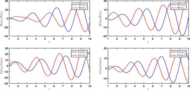
Figure 1. The curves of the variables u1, v1, u2, v2 without the controller.
Then, we will consider the PS of systems (22) and (23) under the controller (9). It is easy to verify that Assumption 1 holds and ${F}_{j}={G}_{j}=\tfrac{2}{3}$, for j = 1, 2. Through calculating (10) of theorem 1, we can obtain that k1 > 1.7, k2 > 1.7, η1 > 10.9060, η2 > 13.0343, ρ1 > 7.5345, ρ2 > 10.776, and σ1 > 12.7906, σ2 > 9.0780. So we choose k1 = 1.71, k2 = 1.71, η1 = 10.91, η2 = 13.04, ρ1 = 7.54, ρ2 = 10.78, and σ1 = 12.80, σ2 = 9.08. From theorem 1, systems (22) and (23) can reach the PS under the controller (9), which can be also seen in figure 2.
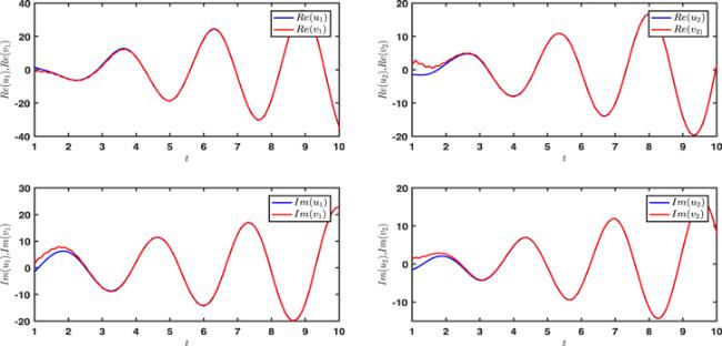
Figure 2. The curves of the variables u1, v1, u2, v2 with the controller.

5. Conclusion

In this paper, we have studied the PS problem of CVINNs with multi-proportional delays by the non-separation method. In order to realize the PS of the addressed system, we have involved the exponential transformation, obtained the power exponential term via fully utilizing some inequality techniques, and solved the main difficulty based on the designed suitable controller and Lyapunov function method. Then, we obtained a simple sufficient condition for PS. Finally, we have provided a numerical simulation example to verify the validity of our work. In the following work, we will focus on other synchronization phenomena of CVINNs, such as module-phase synchronization, projective synchronization, combination synchronization, and so on.

This work was supported in part by the National Natural Science Foundation of China (61503222, 62173214), in part by the Natural Science Foundation of Shandong Province of China (ZR2021MF100), in part by the Research Fund for the Taishan Scholar Project of Shandong Province of China, in part by the Science and Technology Support Plan for Youth Innovation of Colleges and Universities of Shandong Province of China (2019KJI005), and in part by the SDUST Research Fund.

1
Zeng X Wen S Zeng Z Huang T 2018 Design of memristor-based image convolution calculation in convolutional neural network Neural Comput. Applic. 30 503 508

DOI

2
Yang J Wang L Wang Y Guo T 2017 A novel memristive Hopfield neural network with application in associative memory Neurocomputing 227 142 148

DOI

3
Tani J 1996 Model-based learning for mobile robot navigation from the dynamical systems perspective IEEE Trans. Syst., Man, Cybern., Part B 26 421 436

DOI

4
Yang B Wang J Wang J 2017 Stability analysis of delayed neural networks via a new integral inequality Neural Netw. 88 49 57

DOI

5
Velmurugan G Rakkiyappan R Cao J 2016 Finite-time synchronization of fractional-order memristor-based neural networks with time delays Neural Netw. 73 36 46

DOI

6
Zhang Z Wei X Wang S Lin C Chen J Fixed-time pinning common synchronization and adaptive synchronization for delayed quaternion-valued neural networks IEEE Trans. Neural Netw. Learn. Syst.

DOI

7
Babcock K L Westervelt R M 1986 Stability and dynamics of simple electronic neural networks with added inertia Physica D: Nonlinear Phenom. 23 464 469

DOI

8
Babcock K L Westervelt R M 1987 Dynamics of simple electronic neural networks Physica D: Nonlinear Phenom. 28 305 316

DOI

9
Angelaki D Correia M 1991 Models of membrane resonance in pigeon semicircular canal type II hair cells Biol. Cybern. 65 1 10

DOI

10
Lakshmanan S Prakash M Lim C P Rakkiyappan R Balasubramaniam P Nahavandi S 2018 Synchronization of an inertial neural network with time-varying delays and its application to secure communication IEEE Trans. Neural Netw. Learn. Syst. 29 195 207

DOI

11
Long C Zhang G Zeng Z Hu J 2021 Finite-time lag synchronization of inertial neural networks with mixed infinite time-varying delays and state-dependent switching Neurocomputing 433 50 58

DOI

12
Hu J Wang J 2012 Global stability of complex-valued recurrent neural networks with time-delays IEEE Trans. Neural Netw. Learn. Syst. 23 853 865

DOI

13
Kumar A Das S Yadav V K Rajeev 2021 Global quasi-synchronization of complex-valued recurrent neural networks with time-varying delay and interaction terms Chaos Solitons Fractals 152 111323

DOI

14
Zhang Z Liu X Zhou D Lin C Chen J Wang H 2018 Finite-time stabilizability and instabilizability for complex-valued memristive neural networks with time delays IEEE Trans. Syst., Man. Cybern., Syst. 48 2371 2382

DOI

15
Popa C A 2020 Global μ-stability of neutral-type impulsive complex-valued BAM neural networks with leakage delay and unbounded time-varying delays Neurocomputing 376 73 94

DOI

16
Duan L Shi M Huang C Fang X 2021 Synchronization in finite-/fixed-time of delayed diffusive complex-valued neural networks with discontinuous activations Chaos Solitons Fractals 142 110386

DOI

17
Xiong K Yu J Hu C Jiang H 2020 Synchronization in finite/fixed time of fully complex-valued dynamical networks via nonseparation approach J. Franklin Inst. 357 473 493

DOI

18
Feng L Yu J Hu C Yang C Jiang H 2020 Nonseparation method-based finite/fixed-time synchronization of fully complex-valued discontinuous neural networks IEEE Trans. Cybern. 51 3212 3223

DOI

19
Wang S Zhang Z Lin C Chen J 2021 Fixed-time synchronization for complex-valued BAM neural networks with time-varying delays via pinning control and adaptive pinning control Chaos Solitons Fractals 153 111583

DOI

20
Xiao Q Huang T Zeng Z 2022 On exponential stability of delayed discrete-time complex-valued inertial neural networks IEEE Trans. Cybern. 52 3483–94

DOI

21
Iswarya M Raja R Cao J Niezabitowski M Alzabut J Maharajan C 2022 New results on exponential input-to-state stability analysis of memristor based complex-valued inertial neural networks with proportional and distributed delays Math. Comput. Simulat. 201 440 461

DOI

22
Tang Q Jian J 2019 Global exponential convergence for impulsive inertial complex-valued neural networks with time-varying delays Math. Comput. Simulat. 159 39 56

DOI

23
Tang Q Jian J 2018 Matrix measure based exponential stabilization for complex-valued inertial neural networks with time-varying delays using impulsive control Neurocomputing 273 251 259

DOI

24
Li X Fang J A Huang T 2022 Event-triggered exponential stabilization for state-based switched inertial complex-valued neural networks with multiple delays IEEE Trans. Cybern. 52 4585–95

DOI

25
Li X Huang T 2021 Adaptive synchronization for fuzzy inertial complex-valued neural networks with state-dependent coefficients and mixed delays Fuzzy Sets Syst. 411 174 189

DOI

26
Long C Zhang G Hu J 2021 Fixed-time synchronization for delayed inertial complex-valued neural networks Appl. Math. Comput. 405 126272

DOI

27
Yu Y Zhang Z Zhong M Wang Z 2022 Pinning synchronization and adaptive synchronization of complex-valued inertial neural networks with time-varying delays in fixed-time interval J. Franklin Inst. 359 1434 1456

DOI

28
Guo R Xu S Ma Q Zhang Z 2022 Fixed-time synchronization of complex-valued inertial neural networks via nonreduced-order method IEEE Syst. J. 16 4974–82

DOI

29
Guo R Lu J Li Y Lv W 2021 Fixed-time synchronization of inertial complex-valued neural networks with time delays Nonlinear Dyn. 105 1643 1656

DOI

30
Yu Y Zhang Z 2022 State estimation for complex-valued inertial neural networks with multiple time delays Mathematics 10 1725

DOI

31
Long C Zhang G Zeng Z Hu J 2022 Finite-time stabilization of complex-valued neural networks with proportional delays and inertial terms: A non-separation approach Neural Netw. 148 86 95

DOI

32
Wei X Zhang Z Lin C Chen J 2021 Synchronization and anti-synchronization for complex-valued inertial neural networks with time-varying delays Appl. Math. Comput. 403 126194

DOI

33
Yu J Hu C Jiang H Wang L 2020 Exponential and adaptive synchronization of inertial complex-valued neural networks: A non-reduced order and non-separation approach Neural Netw. 124 50 59

DOI

34
Zhou L Zhao Z 2020 Exponential synchronization and polynomial synchronization of recurrent neural networks with and without proportional delays Neurocomputing. 372 109 116

DOI

35
Mao X 1992 Almost sure polynomial stability for a class of stochastic differential equations Quart. J. Math. 43 339 348

DOI

36
Santos M L Rocha M P C Gomes S C 2010 Polynomial stability of a coupled system of wave equations weakly dissipative Appl. Anal. 86 1293 1302

DOI

37
Zhou L Zhao Z 2020 Asymptotic stability and polynomial stability of impulsive Cohen-Grossberg neural networks with multi-proportional delays Neural Process. Lett. 51 2607 2627

DOI

38
Zhang Y Zhou L 2022 Novel global polynomial stability criteria of impulsive complex-valued neural networks with multi-proportional delays Neural Comput. Applic. 34 2913 2924

DOI

39
Hien L V Son D T 2015 Finite-time stability of a class of non-autonomous neural networks with heterogeneous proportional delays Appl. Math. Comput. 251 14 23

DOI

40
Li L Chen W Wu X 2021 Global exponential stability and synchronization for a novel complex-valued neural networks with proportional delays and inhibitory factors IEEE Trans. Cybern. 51 2142 2152

DOI

41
Abazari R Kilicman A 2014 Application of differential transform method on nonlinear integro-differential equations with proportional delay Neural Comput. Applic. 24 391 397

DOI

42
Pan W Mu D Wu H Sun Q 2008 Proportional delay differentiation service in web application servers: A feedback control approach, in ISECS International Colloquium on Computing, Communication Control, and Management. 1 600 604

43
Xue Y Chen K Nahrstedt K 2004 Achieving proportional delay differentiation in wireless LAN via cross-layer scheduling Wirel. Commun. Mob. Com. 4 849 866

DOI

44
Huang Z Bin H Cao J Wang B 2018 Synchronizing neural networks with proportional delays based on a class of q-type allowable time scales IEEE Trans. Neural Netw. Learn. Syst. 29 3418 3428

DOI

45
Yang X Song Q Cao J Lu J 2018 Synchronization of coupled Markovian reaction-diffusion neural networks with proportional delays via quantized control IEEE Trans. Neural Netw. Learn. Syst. 30 951 958

DOI

46
Zhou L 2015 Delay-dependent exponential synchronization of recurrent neural networks with multiple proportional delays Neural Process. Lett. 42 619 632

DOI

47
Zong Y Dai X Gao Z 2020 Proportional-integral synchronization for nonidentical wireless packet-coupled oscillators with delays IEEE Transactions on Ind. Electron. 68 11598 11608

DOI

48
Tang R Su H Zou Y Yang X Finite-time synchronization of Markovian coupled neural networks with delays via intermittent quantized control: Linear programming approach IEEE Trans. Neural Netw. Learn. Syst.

DOI

Outlines

/