Excitation spectra of one-dimensional spin-1/2 Fermi gas with an attraction
Jia-Feng Pan
1, 2
,
Jia-Jia Luo
, 3, *
,
Xi-Wen Guan
, 1, 2, 4, *
Expand
1State Key Laboratory of Magnetic Resonance and Atomic and Molecular Physics, Wuhan Institute of Physics and Mathematics, Innovation Academy for Precision Measurement Science and Technology, Chinese Academy of Sciences, Wuhan 430071, China
2Department of Fundamental and Theoretical Physics, Research School of Physics, Australian National University, Canberra ACT 0200, Australia
3 University of Chinese Academy of Sciences, Beijing 100049, China
4 NSFC-SPTP Peng Huanwu Center for Fundamental Theory, Xi'an 710127, China
*Author(s) to whom all correspondence should be addressed.
Using an exact Bethe ansatz solution, we rigorously study excitation spectra of the spin-1/2 Fermi gas (called Yang–Gaudin model) with an attractive interaction. Elementary excitations of this model involve particle-hole excitation, hole excitation and adding particles in the Fermi seas of pairs and unpaired fermions. The gapped magnon excitations in the spin sector show a ferromagnetic coupling to the Fermi sea of the single fermions. By numerically and analytically solving the Bethe ansatz equations and the thermodynamic Bethe ansatz equations of this model, we obtain excitation energies for various polarizations in the phase of the Fulde–Ferrell–Larkin–Ovchinnikov-like state. For a small momentum (long-wavelength limit) and in the strong interaction regime, we analytically obtained their linear dispersions with curvature corrections, effective masses as well as velocities in particle-hole excitations of pairs and unpaired fermions. Such a type of particle-hole excitations display a novel separation of collective motions of bosonic modes within paired and unpaired fermions. Finally, we also discuss magnon excitations in the spin sector and the application of Bragg spectroscopy for testing such separated charge excitation modes of pairs and single fermions.
Jia-Feng Pan, Jia-Jia Luo, Xi-Wen Guan. Excitation spectra of one-dimensional spin-1/2 Fermi gas with an attraction[J]. Communications in Theoretical Physics, 2022, 74(12): 125802. DOI: 10.1088/1572-9494/ac921a
1. Introduction
The quantum many-body systems manifest abundant physical phenomena, such as Bose–Einstein condensation (BEC), superfluidity, superconductivity, and quantum phase transition, etc, which are regarded as emergent phenomena in modern physics. However, the complexity of many-body systems, involving huge internal degrees of freedom, quantum statistics and interaction, always brings us a formidable task to access their physics of interest. Among the known many-body theories, there are two universal low energy effective theories, i.e. Fermi liquid and Tomonaga–Luttinger liquid (TLL) that capture significant different features of many-body correlations in one dimension (1D) and higher dimensions. Landau Fermi liquid theory [1–3] remarkably describes the metallic behaviour of interacting fermions in 2D and 3D. In this theory the concept of quasiparticles reveals the essence of individual particle excitations close to the Fermi surface in the interacting fermions. In contrast, when the degrees of freedom are reduced to 1D, the elementary excitations in 1D systems strikingly form collective motions of bosons, which are named the TLL in the long-wavelength limit [4, 5]. In the TLL theory, the low energy behaviour of 1D systems can be universally described by the bosonic fields of quantized sound waves or phonons. The early theoretical framework of the TLL for various 1D problems was developed by Lieb and Mattis [6], Haldane [7] and others, see reviews [8, 9]. The TLL has become the main theme in the study of the critical behaviour of 1D many-body systems.
On the other hand, integrable models provide significant insight into the emergent phenomena driven by interactions and quantum statistics in low and higher dimensions [9–11]. The quantum integrability should trace back to H Bethe's work in 1931 when he solved the eigenvalue problem of 1D spin-1/2 Heisenberg chain [12] by writing the wave function of the model as the superposition of all possible plane waves. It was over 30 years after Bethe's work that this method was coined as the BA (Bethe ansatz) by C N Yang and C P Yang in their series of publications in the mid-60s [13–15]. Using Bethe's method, Lieb and Liniger [16] solved the 1D Bose gas with a δ-function interaction, which is now called the Lieb–Liniger model. In 1964 Mcguire [17] studied the 1D Fermi gas with the δ-function interaction by considering the exact solution of one spin-up fermion interacting with N − 1 spin-down fermions. The exact solution of the 1D Fermi gas with arbitrary numbers of spin-up and spin-down particles was solved by Yang [18, 19], while at that time Gaudin [20] obtained the BA solution for the model with a spin balance. This model is now named the Yang–Gaudin model. In C N Yang's seminal work [18], a key discovery of the necessary condition for the BA solvability was surprisingly found. In 1972, Baxter [21] independently showed that such a factorization relation also occurred as the conditions for commuting transfer matrices in 2D vertex models in statistical mechanics. It is now known as the Yang–Baxter equation, i.e. the factorization condition. The Yang–Baxter equation has laid out a profound legacy in a variety of fields in mathematics and physics.
In 1969, Yang and Yang [22] obtained the thermodynamics of the Lieb–Liniger Bose gas at finite temperatures. They found that the thermodynamics of the model can be determined by the minimisation conditions of the Gibbs free energy in terms of the microscopic states determined by the BA equations. Takahashi generalized Yang and Yang's method to deal with the thermodynamics of the 1D Heisenberg spin chain and 1D Hubbard model though introducing string hypotheses [23–27]. He coined the method as the Yang–Yang thermodynamic Bethe ansatz (TBA), see a feature review [28]. Further developments of the TBA approach have been made in the study of universal thermodynamics, Luttinger liquid, spin-charge separation, transport properties and critical phenomena for a wide range of low-dimensional quantum many-body systems, see reviews [11, 29].
In the attractive regime, the Yang–Gaudin model exhibits novel Fulde–Ferrell–Larkin–Ovchinnikov (FFLO) pairing correlation [30, 31], i.e. coexistence of paired and unpaired fermions [32]. Understanding the FFLO pairing behavior in 1D and higher dimensions is still an open challenge in condensed matter physics. The phase diagram of the attractive Fermi gas, consisting of a fully-paired state for an external field is less than the lower critical field Hc1, a fully-polarized state for the magnetic field is greater than an upper critical field Hc2 and the FFLO-like state lies in between the two critical fields, was predicted in [33–35] and experimentally confirmed by R. Hulet's group in [36]. This novel phase diagram reveals striking features of thermodynamics, for instance, universal behaviour of the specific heat [37], the dimensionless ratios, such as the Grüneisen parameter [38] and Wilson ratios [39, 40]. The dark-soliton-like excitations in the Yang–Gaudin gas of attractively interacting fermions and the Lieb–Liniger gas [41, 42] shed light on the nonlinear effects of many-body correlation. Nevertheless, one expects that the elementary excitations in this attractive Yang–Gaudin model would provide significant collective nature of multi-component TLLs with pairing and depairing in thermodynamics and dynamic response functions. This is the major research of the following study in this paper.
In section 2, we will introduce the BA equations and TBA equations, which will be used to accomplish our study of the excitation spectra of the Yang–Gaudin model with an attraction. In section 3, we will present the particle-hole excitation spectra in paired and unpaired fermi seas. In section 4, we will analytically derive dispersion relations with band curvature corrections, effective mass and sound velocities of pairs and unpaired fermions for the Yang–Gaudin model with polarizations in a strong coupling regime. In section 5, we will discuss multiple particle-hole excitations and the magnon excitations in the FFLO-like phase. The last section remains for our conclusion and discussion.
2. Yang–Gaudin model with an attractive interaction
2.1. Bethe ansatz equations and string hypotheses
The 1D two-component Fermi gas with a delta-function interaction is called the Yang–Gaudin model [18–20]. Its Hamiltonian is given by
where N is the number of fermions, N↓ is the number of down-spin fermions, H is the external magnetic field, c < 0 for attractive interaction, and herewith we set ℏ2 = 2m = 1. We always choose an upward magnetic field so that spin-down fermions are less than spin-up ones. As a result, each spin-down fermion can be paired with a spin-up fermion and form a bounded state. While the remaining spin-up fermions are unpaired and in a polarized state. Denote the number of paired fermions as M, then that of unpaired fermions is N − 2M.
The quasimomenta {kj} of the fermions and the rapidities {Λα} of the spin-down fermions are given by the BA equations
for j = 1, 2, ⋯ ,N and α = 1, 2, ⋯ ,N↓, where $e\left(x\right)=\exp \left({\rm{i}}\pi -2{\rm{i}}\arctan x\right)$.
Takahashi [23–27] introduced the following spin string hypotheses for the root patterns of the BA equations (2):
i
(i) Complex Λ↓α always forms a bound state with several other Λ↓α's. In this set of n-Λ↓α's the real parts are the same and the imaginary parts are (n − 1)ci, (n − 3)ci, ⋯ , − (n − 1)ci for each of them within the accuracy of ${ \mathcal O }(\exp (-\delta N))$, where δ is a positive number. This bound state of n-Λ↓α's forms an n-string. In the following discussion, we will denote each of these complex n-Λ↓α strings as Λαn,j, where j = 1, 2, ⋯ ,n. We suppose that there are Mn-n-strings, and denote the real part of each n-string as Λαn, where α = 1, 2, ⋯ ,Mn. Then we can express the n-string as
(ii)For an attractive interaction c < 0, a pair of quasi-momenta form a charge bound state, namely kα and its complex conjugate ${\bar{k}}_{\alpha }$ have a common real part Λ, i.e.
Supposing that there are M charge bound pairs and $\left(N-2M\right)$ single fermions with the quasi-momenta $\left\{{k}_{j}\right\}$ with j = 1, 2, ⋯ ,N − 2M. Then the BA equations (2) can be rewritten in the following form [26]
Here Jα is the integer (half-odd integer) for N − M odd (even), Ij is the integer (half-odd integer) for M + M1 + M2 + ⋯ even (odd), and Jαn is the integer (half-odd integer) for N − Mn odd (even). Jαn should satisfy the condition
Equation (5) gives quantum numbers Jα, Ij, and Jαn for the charge sector of paired fermions, the charge sector of unpaired fermions, and the spin sector of unpaired fermions, respectively. It turns out that for each pair kα and ${\bar{k}}_{\alpha }$ are given by Λα, representing quasi-momenta of pairs. Whereas kj represents quasi-momenta of N − 2M unpaired fermions and Λαn represents Mn spin wave bound states (the length-n strings).
In the thermodynamic limit, i.e. L, N → ∞ , these quantum numbers could be treated as functions of continuous variables ks, which satisfy
where σ, ρ, σn denote distribution functions of bound pairs, single particles and length-n spin strings, respectively. While ${\sigma }^{h},{\rho }^{h},{\sigma }_{n}^{h}$ denote the distribution functions of their corresponding holes. The continuous k stands for discrete quasi-momenta kj, Λα and Λαn. It follows that the BA equations (2) become as [26]
2.2. Thermodynamical Bethe ansatz equations and thermodynamic quantities
Building on microscopic state energies, we may further define dressed energies of pairs $\varepsilon =T\mathrm{ln}\eta $, single fermions $\kappa =T\mathrm{ln}\zeta $, and length-n strings ${\varepsilon }_{n}=T\mathrm{ln}{\zeta }_{n}$, respectively. Here we denoted the quantities ζ = ρh/ρ, η = σh/σ, and ${\eta }_{n}={\sigma }_{n}^{h}/{\sigma }_{n}$. Minimizing thermodynamic potential Ω ≡ E − TS − AN − HSZ with respect to the densities through equation (9), i.e. δΩ = 0, we may obtain the following TBA equations [26]
where n = 1, …, ∞. In the above equations, T, A and H stand for temperature, chemical potential and magnetic field, respectively. Accordingly, we can give the equation of state, namely the pressure p is given by
The pressure of this system is simply the sum of two terms, the term regarding the paired Fermi sea and another regarding the unpaired sea, respectively. Other thermodynamic quantities can be calculated through the usual thermodynamics relations:
where the last three quantities are the compressibility, magnetic susceptibility, and specific heat.
At the zero temperature T → 0, due to the ferromagnetic ordering, we observe that ηn → ∞ and σn = 0 for n = 1, 2, ⋯ and the TBA equations (12) reduce to
where the superscript ‘−' means the corresponding quantities are the negative parts. Since ϵn− → 0 for n ≥ 1 in the limit T → 0, these equations are referred to the zero temperature dressed energy equations. In this case, the Fermi points B, Q are determined by $\varepsilon \left(B\right)=0$ and $\kappa \left(Q\right)=0$. It turns out that $\varepsilon \left(k\right)$ and $\kappa \left(k\right)$ are monotonically increasing functions of k2. Therefore, B and Q are Fermi surfaces referring to the continuous quasimomentum of paired and unpaired fermions. They can also be determined by the relations
where σn = 0 for the ground state and spin sector is completely gapped.
Moreover, at zero temperature limit T → 0, there exists the phase transition among fully paired phase, fully-polarized phase, partially-polarized phase, and vacuum phase, which will be further studied in section 4.1. The fully paired phase can be regarded as the Bardeen–Cooper–Schrieffer (BCS) like phase, which is expected to manifest the first-type superconductivity. The phase diagram are given in [34, 35, 37, 43]. Fulde and Ferrell [30] and Larkin and Ovchinnikov [31] predicted the exotic superfluid phase, which is now called the FFLO phase. The partially polarized phase in the attractive Yang–Gaudin model is composed of BCS-like pairs and unpaired fermions, presenting a 1D-analogy of the FFLO phase. The FFLO-like phase diagram of the attractive Fermi gas was experimentally confirmed by Hulet's group [44].
3. Spectra of one-particle-hole excitations
3.1. Ground state
Consider the partially polarized phase, where paired and unpaired fermions coexist. The total momentum of the system is given by
Due to the ferromagnetic ordering in the spin sector, the distribution functions σn = 0 with n = 1, 2, ⋯ at the ground state. In other words, there is no particle for the length n-strings, i.e. Mn = 0. Therefore, the spin sector of unpaired fermions does not contribute to the total momentum, i.e. Ks,u = 0 at the ground state.
For the ground state, both paired and unpaired fermions should occupy those lowest-energy states, i.e. states with the lowest absolute quantum numbers (quasi-momenta). Consequently, most contributions of particles to total momentum are neutralized in the sum of positive and negative quantum numbers. The total momentum is not zero only if the distribution of quasi-momenta is not symmetric around the zero quasi-momentum. Figure 1 presents an example of non-zero total momentum, which essentially shows a two-fold degeneration.
Figure 1. Schematic illustration of the two-fold degeneration. IF,a,− and IF,a,+, (or ${I}_{F,b,-}^{\prime} $ and ${I}_{F,b,+}^{\prime} $ ) give respectively the Fermi points of the unpaired (paired) sector. In this case, the particle number is odd while the corresponding quantum number Ijs take half-odd integers. It appears that these quantum numbers cannot distribute symmetrically. Therefore, the total momentum is non-zero and the ground state is two-fold degenerate.
There are totally M paired fermions, whereas Jαs take integers (half-odd integers) for N − M odd (even). Therefore, Jαs are symmetrically distributed if and only if N is even. Similarly, there are N − 2M unpaired fermions, whereas Ijs take integers (half-odd integers) for M + ∑Mn = M are even (odd). Therefore, Ij is symmetrically distributed if and only if N + M is odd, see equation (5). Consequently
where nb = M/L and nu = (N − 2M)/L are particle densities of paired and unpaired sectors, respectively.
Introduce the superscript ‘0' to denote the ground state. Accordingly, the dressed-energies equation (15) and the density distribution functions and equation (17) are respectively written as
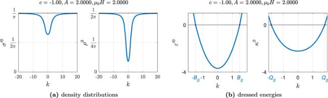
Figure 2. (a) Density distribution functions and (b) dressed energies at zero temperature. (a) For k → ± ∞, the density distributions of paired fermions σ0 and unpaired fermions ρ0 tend to 1/π or 1/(2π), respectively. (b) The dressed energies of paired and unpaired fermions are monotonically increasing with ∣k∣. Therefore, the Fermi points referring to the continuous quasi-momenta can be well defined by the conditions ϵ0(±B0) = 0 and κ0(±Q0) = 0, respectively.
Figure 3. Schematic illustration of the one-particle-hole excitation: moving one particle within the two Fermi points to outside the Fermi sea.
In terms of the additivity of the total momentum in equation (18), we can naturally define the Fermi points, kF,b,± and kF,u,±, referring to the discrete quasimomenta of both paired and unpaired sectors, by maximal and minimal quantum numbers within occupied {Jα} and {Ij}, respectively. For Jα symmetrically distributed, $\left|{k}_{F,b,\pm }\right|=2\pi \left|{J}_{F,\pm }\right|/L=\pi (M-1)/L\approx \pi {n}_{b}$ for a thermodynamical limit, i.e. N, L → ∞; whereas for the asymmetrical case, we still have $\left|{k}_{F,b,+}\right|=\pi (M-1\pm 1)/L\approx \pi {n}_{b}$ and $\left|{k}_{F,b,-}\right|=\pi (M-1\mp 1)/L\approx \pi {n}_{b}$, where the additional terms ± π/L emerging due to the two-fold degeneration are negligible for the thermodynamical limit. With similar regard, we have kF,u,± = 2πIF,± ≈ πnu for the Fermi points referring to the unpaired fermions. The Fermi points are referred to the conditions ${\varepsilon }^{0}\left({Q}_{0}\right)=0$ and ${\sigma }^{0}\left({B}_{0}\right)=0$, where B0 and Q0 are different from the quasimomenta kF,b,± and kF,u,± of pairs and unpaired fermions.
3.2. Sound velocity and effective mass for one-particle-hole excitation
Consider one particle-hole excitation of unpaired fermions, where one quasiparticle with a quasimomentum kh inside the Fermi points is excited outside the Fermi points with a quasimomentum kp (see figure 3), i.e.
Define $\bar{\rho }\left(k\right)=\rho \left(k\right)+{\rho }^{h}\left(k\right)$, which is changed by ${\rm{\Delta }}\bar{\rho }\left(k\right)$ after the excitation. Since there is exactly one excited hole inside the Fermi points and one quasiparticle outside,
Therefore, ${\rm{\Delta }}\bar{\rho }\left(k\right)$ is the sum of two δ-functions, −δ(k − kh)/L and δ(k − kp)/L. Also, it defines $\bar{\sigma }\left(k\right)=\sigma \left(k\right)+{\sigma }^{h}\left(k\right)$. Consequently, the distribution functions equation (17) is rewritten as
where B± and Q± are the fermi surfaces of the excited system. In the TBA approach, the equilibrium state of the system is determined by minimizing free energy Ω = E − μN − TS, so, the excited free energy is
For the Yang–Gaudin model with repulsive interactions, it is proved [45] that the excited energy can be expressed in the dressed energies. Using a similar method and after a lengthy calculation, we may obtain excitation spectra in the attractive Fermi gas (see appendix A.1), namely
Since the particle numbers N, M, and Mn are conserved, the configurations of quasimomenta remain unchanged. In other words, if the positions of quasi-momenta are originally symmetrically (asymmetrically) distributed with respect to the zero-point, they are still symmetrically (asymmetrically) distributed after an excitation. Therefore, the excited momentum of the systems is equal to the quasi-momentum of the excited particle, namely,
By giving all possible kp and kh (λp and λh), one can obtain one-particle-hole excitation of unpaired (paired) fermions. Accordingly, the spectrum can be plotted for certain choices of parameters {c, A, μ0H}, see figure 4.
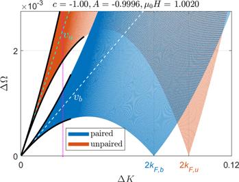
Figure 4. One-particle-hole excitation spectra of paired (blue) and unpaired (dark brown) fermions. kF,b (vb) and kF,u (vu) are the Fermi momenta (velocities) of paired and unpaired fermions, respectively. For small ΔK, the paired and unpaired excitation spectra tend to the linear dispersions with different velocities vb and vu, which are indicated by the white and green dashed lines, respectively. The curvature effects of these dispersions can be conceived from the effective masses which were further studied in section 4. In this figure, we set c = −1.00, A = −0.9996, μ0H = 1.0020 for our numerical calculation with the dispersions represented by equations (24)–(26).
Apparently, there exists charge–charge separation at least for small ΔK. The particle-hole continuum in the long-wavelength limit (ΔK → 0) manifests the free fermion-like dispersion. Two thresholds of the excitation spectrum (black solid lines in figure 4) reveal a curvature effect. The first-order corrections to the linear dispersions of paired and unpaired fermions can define the effective masses ${m}_{b}^{* }$ and ${m}_{u}^{* }$ as well as the sound velocities, vb and vu, see cyan and white dashed lines in figure 4, respectively. We will analytically calculate them in section 4. This is meaningful because it is much easier to measure specific signals referring to specific quantities, such as the sound velocities, which characterize a spectrum than to measure a whole spectrum in the experiment. By tuning the parameters {c, A, μ0H}, the ratio of sound velocities and Fermi surface of the two sectors are controllable, as shown in figure 5.
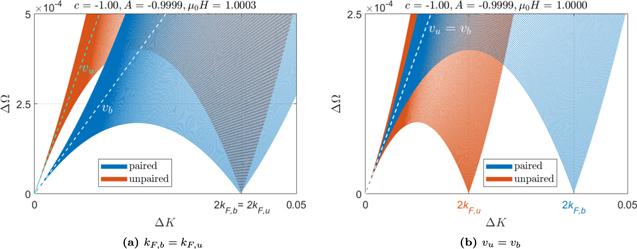
Figure 5. One-particle-hole excitation spectra of paired (blue) and unpaired (dark brown) fermions with kF,b = kF,u (a) and vu = 2vb (b). In (a), we set c = −1.00, A = −0.9999, μ0H = 1.0003 for our numerical calculation with the equations (24)–(26); in (b), we set c = −1.00, A = −0.9999, μ0H = 1.0003. These parameters are artificially selected, which we will explain in section 4.
4. Analytical results
4.1. Strong coupling limit in partially polarized phase
In general, analytical expressions of physical quantities are hardly obtained from the BA equations unless in certain extreme limits. Usually, one considers the weak and strong coupling limits, $\left|c\right|\ll n$ and $\left|c\right|\gg n$ in 1D ultracold atomic systems. The coupling strength $\left|c\right|/n$ can be experimentally tuned from weak to strong by controlling the 3D scattering length near the Feshbach resonance, i.e.
where g1D is the effective inter-component interaction, a3D is the 3D scattering length, a⊥ is the transverse oscillator length. For our convenience, we denote the dimensionless coupling strengths $\gamma =\left|c\right|/n$, ${\gamma }_{b}=\left|c\right|/{n}_{b}$, and ${\gamma }_{u}=\left|c\right|/{n}_{u}$. What below are the derivations of analytical results of physical quantities for the strong coupling regime, γ ≫ 1.
In the grand canonical ensemble, quantum phase transitions take place at zero-temperature, which have already been studied in both the canonical ensemble and the grand canonical ensemble [34, 35, 37, 43]. Here we discuss analytical results in the grand canonical ensemble, where the parameters {c, A, μ0H} are our driving parameters. For example, the phase diagram and interaction strengths can be given in μ–H plane, see figures 6 and 7.
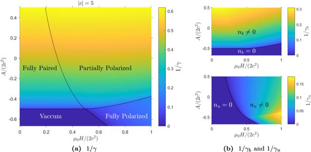
Figure 6. Phase diagrams represented by dimensionless particle densities 1/γ, 1/γb and 1/γu. Here dimensionless quantities A/(2c2) and μ0H/(2c2) are used as variables, where 2c2 is the binding energy. The black lines indicate the phase boundaries, which are obtained from the two diagrams in (a). For the partially polarized phase, the strong coupling γ ≫ 1 near the quartet point. Clearly, according to (b), the boundaries of each phase (black lines) in (a) are given at the boundaries of zero- or nonzero-particle densities of paired and unpaired sections. The phase boundaries in (a) can also be determined by equation (15).
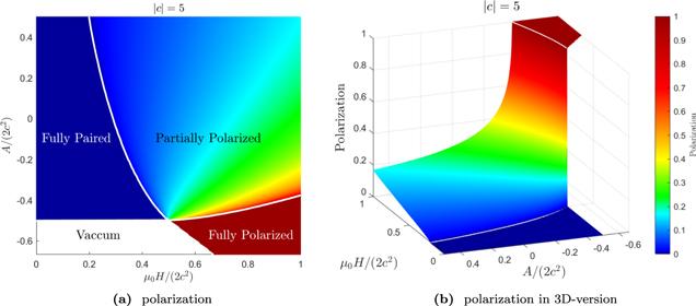
Figure 7. Phase diagram is represented by polarization. In (a), the white lines give the phase boundaries. In (b), the polarization varies drastically in the vicinity of the quartet point.
From figure 6, we observe that the strong coupling γ ≫ 1 (regions plotted in dark blue) can be reached in the vicinity of the edge of the vacuum phase. In the partially polarized (FFLO-like) phase, the strong coupling regime locates near the quartet point A/c2 = −1 and μ0H/c2 = 1. If we define the effective chemical potentials of both sector Ab = A + c2 and Au = A + μ0H, the strong coupling regime meets the condition Ab ≪ c2 and Au ≪ c2.
In figure 7(a), we plot the polarization in the μ–H plane for a fixed value of interaction strength. From figure 7(b), we observe the polarization P = nu/(2nb + nu) varies drastically in the vicinity of the quartet point. Therefore, it might come into the expression of the band curvature corrections of sound velocities and effective masses for the strong coupling.
4.2. Sound velocity and effective mass in one-particle-hole excitation spectrum
In this section, we will derive the exact dispersions of particle-hole excitations in both paired and unpaired fermions. We first derive the dispersion of bound pairs in the long-wavelength limit, i.e. we derive the linear dispersion with a curvature correction. Consequently, we can obtain the sound velocities and effective masses in terms of dressed energies and the density distribution functions. For a one-particle-hole excitation near the Fermi point B of the bound pairs, the excited energy and momentum are given by
In the long-wavelength limit, the excitation is near the Fermi point, i.e. Δk ≪ 1. Therefore, the excited energy and momentum can be expanded at k = B. Namely,
expressed up to the second order of ΔKb. From this relation, we read off the sound velocity and effective mass of the one-particle-hole excitation in the paired Fermi sea as
The obtained relations for velocities and effective masses (33) and (36) are very convenient to carry out numerical calculations, see figure 4.
For a strong coupling, i.e. ∣c∣ ≫ 1, we may directly use the dressed energies equation (15) and the distribution functions equation (17) to determine the dispersion relations characterized by the sound velocities and effective masses. To this end, we first calculate Fermi momenta B and Q in terms of particle densities nu, nb with our chosen parameters {c, A, μ0H} (i.e. [Ab, Au]). For the strong coupling, we may expand the kernels a1(k) and a2(k) up to the first order of 1/c, the distribution functions equation (17) thus become
Consequently, according to equations (39) and (41), we built up the relations between the particle densities and our chosen parameters {c, A, μ0H} through the Fermi points B and Q.
Now we can rewrite the expressions of the sound velocities and effective masses following the expressions equations (33) and (36) for the strong coupling regime. To determine vb and ${m}_{b}^{* }$ given by equation (33), we first calculate $\varepsilon ^{\prime} (B)$ and σ(B) and their derivatives. Equation (15), $\varepsilon ^{\prime} (B)$ is given by
where we ignored the order 1/c2, for example, the leading order of dan(k)/dk is ${ \mathcal O }(1/{c}^{3})$ in the strong coupling limit. Similarly, we can have $\varepsilon ^{\prime\prime} \left(B\right)=4+{ \mathcal O }(1/{c}^{4})$. Whereas the distribution function $\sigma \left(B\right)$ can be obtained by substituting equations (37) into (17), namely,
While its derivative $\sigma ^{\prime} \left(B\right)\sim { \mathcal O }\left(1/{c}^{3}\right)$ is negligible. By substituting $\varepsilon ^{\prime} (B)$ and σ(B) and their derivatives into equation (33), we may express vb and ${m}_{b}^{* }$ with respect to Fermi momenta B and Q
Furthermore, owing to equations (39) and (41), we replace γb and γu in equations (45) and (47) with γ and the polarization P or the ratio between two effective chemical potentials Ab and Au. Since the polarization is defined by P = nu/n, we have γ/γb = nb/n = (1 − P)/2 and γ/γu = nu/n = P, which allows us to express the sound velocities and effective masses as a function of P. Alternatively, we would like to express the sound velocities and effective masses in terms of Ab and Au. Since they are directly related to our controllable parameters {c, A, μ0H}. According to equations (39) and (41), we have
We denote the ratio of effective chemical potential as Au/Ab = α2 for our convenience in analysis. Using the polarization P and the ratio α, we can rewrite equations (45) and (47) as
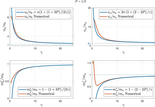
which are confirmed by numerical results in figure 8, where we set the polarization P = 1/5 (i.e. α = 1). According to equation (48) and the last equation (49), the ratio between two sound velocities is simply given by vu/vb = 2nu/nb = α up to the order of 1/c2, which provides physical insight into the sound velocities in figure 5, where our chosen parameters {c, A, μ0H} indicate a strong coupling with α = 2 and α = 1, respectively. Furthermore, since kF,b ≈ πnb and kF,u ≈ πnu (illustrated at the end of section 3.1), we have kF,u/kF,b =α/2, which gives a special ratio between two Fermi points in figure 5.
Figure 8. Variation of sound velocities, vb and vu, and effective masses, ${m}_{b}^{* }$ and ${m}_{u}^{* }$ versus the dimensionless interaction strengths γ. The polarization is fixed to be P = 1/5 with γ = 10. The analytical (blue) equation (49) are agreeable with the numerical (red) results which are plotted with respect to equations (33) and (36).
So far, we derived the sound velocities and effective masses of paired and unpaired fermions starting from the zero-temperature TBA equations. For the repulsive case, it is proved [45] that these quantities can be derived from the BA equations; by a similar method, one can prove that this works for the attractive case as well (see appendix A.2 for detailed procedure). This is reasonable since the TBA equations are derived from the BA equations.
The sound velocities and effective masses can effectively characterize the spectra of one-particle-hole excitation. Therefore, these quantities can be regarded as evidence and provide convenience to verify the separation of collective motions within paired and unpaired charges at zero temperature. This kind of charge–charge separation can even be characterized at non-zero but low temperature. According to the relations given by equations (33) and (36), the zero-temperature subtraction for low-temperature free energy density can be expressed by (see appendix A.3 for proof)
which is simply the addition of contribution of paired and unpaired sections. This additivity manifests the independent character and separation of paired and unpaired bosonic modes. Moreover, the T2 dependence given by the low-temperature pressure correction shows a typical linear dispersions feature. The specific heat can also be obtained by its definition, i.e.
which preserves the additivity and describes the novel charge–charge separation as well at low temperature.
5. Excitations other than single particle-hole
In this section, we will consider excitations other than the one particle-hole excitation, such as excitations of multiple particle-holes, breaking and forming pairs, as well as length-n string excitations.
5.1. Multiple particle-hole excitations
In the case of exciting Nb paired fermions and Nu unpaired fermions, like what we did in equation (22), introducing 2Nb +2Nuδ-functions, ${\sum }_{i=1}^{{N}_{b}}[-\delta \left(k-{k}_{h,i}\right)+\delta \left(k-{k}_{p,i}\right)]\,/L+{\sum }_{j=1}^{{N}_{u}}[-\delta \left(k\,-\right.$ $\left.{k}_{h,j}\right)+\delta \left(k-{k}_{p,j}\right)]/L$ into the distribution functions equation (17), one can prove that the excitation energy momentum is given by their summation of one-particle-hole excitation ones, respectively
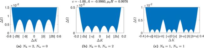
The calculation is essentially similar to that for one-particle-hole dispersion. Here we do not wish to present the calculation in detail. Figure 9 shows three examples for various choices of the numbers Nb and Nu.
Figure 9. Two-particle-hole excitations spectra. The numbers of excited particle holes in paired and unpaired sectors. Figures (a)–(c) show particle-hole excitations for different Nb and Nu. Here we denote $[\alpha b+\beta u]\equiv :2\left(\alpha {k}_{F,b}+\beta {k}_{F,u}\right)$. In this figure, we set c = −1.00, A = −0.9960, μ0H = 0.9976 for our numerical calculation with the dispersions represented by equation (52).
5.2. Excitations by pairing and depairing without exciting any n-string
For the case of breaking Nub pairs, we create Nub holes in the paired Fermi sea while adding 2Nub fermions in the unpaired sea, see figure 10. For the case of forming Nbu pairs, we create 2Nbu holes in the unpaired Fermi sea and add Nbu pairs in the paired Fermi. In comparison with the ground state, for breaking Nub pairs, while forming Nbu pairs, the particle numbers are given by
respectively, where kp1,i, kp2,i, kh1,i, and kh2,i stand for the excited quasimomenta of unpaired particles and holes. As we did in equation (22), substitute the δ-functions (53) into the distribution functions equation (17). By taking a similar calculation to that of the single particle-hole excitation, the excited energy of multiple pair-forming and breaking is given by
The total momentum for this excitation depends on not only the quasimomenta of exited holes and particles but also the numbers of breaking pairs and forming pairs Nub and Nbu. The parity of quasimomenta of pairs in such a type of excitations does not change because it only depends on N = NG (see equation (19)). Meanwhile the parity of quasimomenta of unpaired fermions is changed since it depends on N + M = NG + MG − Nub + Nbu. Therefore, an additional phase shift is caused due to the change of parity, namely,
We see that odd $\left\{{N}_{{ub}}-{N}_{{bu}}\right\}$ gives a two-fold-degenerate excited state. In figure 11 we present excitation spectra of breaking or forming one pair. Obviously, the spectra are more complicated due to the two-fold degeneracy.
Figure 11. Excited spectrum of breaking or forming one pair. The excitation spectra show two-fold degeneracy in breaking a pair and forming a pair. Here we denote $[\alpha b+\beta u]\equiv :2\left(\alpha {k}_{F,b}+\beta {k}_{F,u}\right)$. We set c = −1.00, A = −0.9000, μ0H = 1.0100 for our numerical calculation with the dispersions equations (54) and (55).
5.3. n-strings excitations
Now we consider excitations by flipping spins in the unpaired fermions without forming pairs. According to equation (12), the dressed energy and distribution function in the spin sector at the ground state are given by
For the ground state, all spin strings are unoccupied at zero temperature. The dressed energies and distribution functions for n-strings with n = 1, 2, 3 are plotted in figure 12(a).
Figure 12. (a) Dressed energies ${\varepsilon }_{n}^{0}\left(k\right)$ and distribution functions ${\sigma }_{n}^{0}\left(k\right)$ for n = 1, 2, 3. The dressed energies ${\varepsilon }_{n}^{0}\left(k\right)$ tend to 2nμ0H for k → ±∞. For the ground state, ${\sigma }_{n}^{0}$ gives the distribution of holes because of Mn=0. (b) Excitation spectra of the spinon-bound-states. For a single length-n string excitation, double degeneracy spectrum is observed (left). The right figure shows the continuum spectra of two length-1 spinons.
For simplicity, consider the case of exciting one length-l string by flipping unpaired fermions, i.e. Ml = Ml,G + 1 = 1 and Mn = 0 for n ≠ l. The quantum numbers of the spin setor Jαn are integer (half-odd integer) for N − Mn odd (even), and satisfy equation (7). Therefore, for the ground state, Jαn are confined by the condition
that indicates N − 2M − 2n holes for n ≤ ℓ, N − 2M − 2ℓ holes for n > ℓ and one occupation of length-ℓstring for n = ℓ. By introducing $\delta \left(k-{\lambda }_{{\ell }}\right)/L$ representing the excited ℓ-string into the distribution functions, we have
where we denoted ${\bar{\sigma }}_{n}={\sigma }_{n}+{\sigma }_{n}^{h}$, and we define Bn by ${\bar{\sigma }}_{n}({B}_{n})=0$. The excited free energy density is thus given by
where the last term equals zero since all strings are unoccupied at the ground state. By the calculations similar to that of the excited energy of one particle-hole excitation (see appendix A.1), the excited energy of the length-ℓstring excitation is given by
In the case of exciting one length-ℓstring, the parity of quasimomentum kj for the unpaired charge sector is changed due to its dependence on the quantum numbers $M+{\sum }_{n=1}^{\infty }{M}_{n}$. Therefore, apart from the contribution of the excited string, there is an additional term in the total excited momentum attributed to the momentum change of the unpaired sector, namely,
In the case of excitations of ${M}_{n}^{\mathrm{ex}}$ length-n strings, i.e. ${M}_{n}={M}_{n}^{\mathrm{ex}}$, we introduce the excitation function ${\sum }_{n=1}^{\infty }{\sum }_{i=1}^{{M}_{n}}\delta \left(k-{\lambda }_{n,i}\right)/L$ in the BA equations. One can prove that the excited energy is the sum of those of individual n-string excitation, while the excited energy has an additional term due to the change of configurations in the unpaired quasimomenta
The excitation spectra of one and two n-strings with n = 1, 2, 3 are given in figure 12(b), respectively. These spectra are gapped with a magnitude of 2nμ0H over the ground state. Since a certain number of unpaired fermions are flipped, these excitations should be regarded as magnon excitations that show a ferromagnetic coupling in the unpaired sector. The string structure of these kinds has been confirmed in the experiment [46].
6. Conclusion and discussion
We have rigorously studied the excitation spectra of the Yang–Gaudin model with an attractive interaction. For the one particle-hole excitations in paired and unpaired fermions, the spectra apparently manifest a novel separation of collective motions of bosonic modes, i.e. the pairs-unpaired-fermions separation, which can be regarded as evidence for the existence of the FFLO-state. We further analytically characterized this separation by calculating the curvature corrections to the linear dispersions of both paired and unpaired sections for a small momentum and a strong coupling regime. We have determined the sound velocities and effective masses in these dispersions, and compared them with numerical results. We have shown that the free energy and the specific heat of the system can be simply expressed in a sum of inverse sound velocities of paired and unpaired Fermi seas at low temperatures, reflecting the universal thermodynamics of TLLs. We have also studied other types of excitations, such as breaking or forming a pair and length-n string excitations in the spin sector, in order to understand subtle novel pairing and depairing states. Here the gapped length-n string excitations manifest a ferromagnetic coupling in the unpaired Fermi sea, i.e. magnon excitations.
Building on our results obtained, we expect to further study dynamical correlation functions for the charge–charge separation theory of FFLO states. According to the linear response theory [47], one can measure the spectra of pairing and depairing in the system by imposing a perturbation onto the system and observing their linear responses. Bragg spectroscopy [48] is one of the common experimental tools used to measure the many-body correlation. Using Bragg spectroscopy, the recent experiment [49] conducted by Hulet's group at Rice University has confirmed the spin-charge separation theory of TLLs in the 1D repulsive Fermi gas. In Bragg spectroscopy, 6Li atoms are trapped in 1D-tubes and two beams of different orientations are imposed onto the tubes. Due to the disturbance of the two beams, initially symmetrically distributed particles distribute asymmetrically in the tube. The dynamic structure factor (DSF) S(q, ω), usually defined as the density-density correlation, is related to the change of the total momentum as ΔP ∝ [S(q, ω) − S(−q, −ω)]. Therefore, the DSF is a measurable quantity in the experiment with both repulsive and attractive Fermi gases. Moreover, at low-energy excitations, the maximum (peak) of the DSF is related to the sound velocity, namely, the corresponding peak frequency is given by ωp = vcq, and it is independent of the effective mass. Accordingly, different sound velocities of the paired and unpaired fermions can be observed by the Bragg spectroscopy, showing the subtle nature of the FFLO states in 1D.
Appendix
A.1. Express excited energies in dressed energies
First, introduce two useful formulas.
Formula 1: Any two groups of the analytical functions of the form
One can prove it by multipy $\eta \left(k\right)$ and $f\left(k\right)$.
Formula 2: For any even analytical function $f\left(k\right)$ integrated between $\left[{k}_{-},{k}_{+}\right]$,where k+ = k0 + ΔQ+, k− = −k0 +ΔQ− (for ΔQ± small enough), it can be expanded with ΔQ±, i.e.
where ${\rm{\Delta }}\bar{\rho }\left(k\right)=\bar{\rho }\left(k\right)-{\rho }^{0}\left(k\right)$, ${\rm{\Delta }}\bar{\sigma }\left(\lambda \right)=\bar{\sigma }\left(\lambda \right)-{\sigma }^{0}\left(\lambda \right)$, and formula 2 is used in the last step. Since the particle number does not change, i.e. N − NG = 0, we directly have
Since ${\varepsilon }^{0}\left({B}_{0}\right)={\varepsilon }^{0}\left(-{B}_{0}\right)=0$ and ${\kappa }^{0}\left({Q}_{0}\right)={\kappa }^{0}\left(-{Q}_{0}\right)=0$, we directly obtain
Together with equation (25), the dispersion of one-particle-hole excitation of the unpaired fermions is obtained.
The dispersion of paired fermions can be acquired in the same way. In brief, we again introduce two δ-functions $-\delta \left(\lambda -{\lambda }_{h}\right)+\delta \left(\lambda -{\lambda }_{p}\right)$ as ${\rm{\Delta }}\bar{\sigma }(\lambda )$. Accordingly, the distribution functions are
Using the same technique as that for unpaired fermions, one can essentially acquire the excited exergy given by equation (26).
In general, we can have excitations of 2Nb particle-holes in the paired sector and 2Nu in the unpaired sector simultaneously. One can easily prove that the multiple particle-hole excitations are simply a summation of single-particle-hole excitations with 2Nu + 2Nbδ-functions introduced into the distribution functions, i.e. ${\sum }_{i=1}^{{N}_{b}}[-\delta \left(k-{k}_{h,i}\right)+\delta \left(k-{k}_{p,i}\right)]/L$ and ${\sum }_{j=1}^{{N}_{u}}[-\delta \left(k-{\lambda }_{h,j}\right)+\delta \left(k-{\lambda }_{p,j}\right)]/L$.
For solely breaking and forming pairs, since there is no excitation of length-n strings, the dispersions are similar to the above ones. The difference is likely that the excited state might be degenerate in this case due to the change of particle numbers of each sector, as described by equation (55).
For excitations of one length-l string, the distribution functions are given by equation (59). Since there is exactly one occupied string, ${\sigma }_{n}(k)=\delta \left(k-{\lambda }_{l}\right)/L$. Then the excited free energy density equation (60) can be rewritten as
Since ${\varepsilon }^{0}\left({B}_{0}\right)+{\varepsilon }^{0}\left(-{B}_{0}\right)=0$ and ${\kappa }^{0}\left({Q}_{0}\right)+{\kappa }^{0}\left(-{Q}_{0}\right)=0$, the first three terms of R.H.S. of the last equation can be rewritten. Namely, we have
Substituting the last equation into equation (A15) we obtain the excited energy equation (61) expressed in the length-ℓ-string dressed energy.
A.2. Sound velocity and effective mass from Bethe ansatz
In section 3.2, we derived sound velocities and effective masses of paired and unpaired fermions from the zero-temperature TBA equations. Here we apply the method of [45] to derive the results from the BA equations in detail.
Since Mn = 0 at the ground state, the logarithm of the BA equations of the two charge sectors are
For the ground state, at the thermodynamic limit, we can expand both equations with coupling strength up to order $\sim { \mathcal O }(1/c)$, the first of which gives
respectively. According to equations (A20) and (A21), the approximation of Λα is independent of the parity of kj. By substituting equation (39) into (A20), we have
where the first term of RHS of the last equation πJα/L equals the quasimomentum of free paired fermions, while the remaining terms emerge from the interactions among fermions.
The total energy and momentum of the paired fermions are given by
where ${\tau }_{b}=\displaystyle \frac{1}{2{\gamma }_{b}}+\tfrac{1}{{\gamma }_{u}}$. For one-particle-hole excitation near the Fermi surface, the quantum number of the excited particle and hole are
where β is chosen to be much smaller than M so that the excitation is taken near the Fermi surface. Therefore, the excited momentum of free paired fermions is
We would like to express this dispersion in free-fermion approximation, with the mass of free-fermion m (set to be 1/2 previously) replaced by the effective mass m* due to the interactions. Namely,
which is the same as the sound velocity and effective mass of unpaired fermions in equations (47).
A.3. Free energy at low temperature
To distinguish quantities at zero-temperature and low-temperature, we introduce the subscript ‘0' indicating zero-temperature. Accordingly, dressed energies at zero-temperature ϵ0 and κ0 given by equation (15); while dressed energies at low-temperature can be expanded with respect to zero-temperature as ϵ = ϵ0 + β and κ = κ0 + γ. Namely, we have
where we omitted the integral intervals (−∞, ∞) for convenience of notation. Since for low-temperature, the integrals on the R.H.S. of the last two equations mostly attribute to the values of integrands near the Fermi momenta B and Q, we replace ϵ(k) and κ(k) with their linear expansions (k − B)ub and (k − Q)uu, respectively, where ub and uu denote $\varepsilon ^{\prime} (B)$ and $\kappa ^{\prime} (Q)$, respectively. Namely, we have
We further denote ${\beta }_{0}(k)=({\pi }^{2}{T}^{2})/(6{u}_{b})\left[{a}_{2}(k-B)+{a}_{2}(k+B)\right]\,+({\pi }^{2}{T}^{2})/(6{u}_{u})\left[{a}_{1}(k-Q)\,+\right.$ $\left.{a}_{1}(k+Q)\right]$ and ${\gamma }_{0}(k)\,=({\pi }^{2}{T}^{2})/(6{u}_{b})\left[{a}_{1}(k-B)+{a}_{1}(k+B)\right]$, so that the last equations can be simplified as
Below we will prove that the last four terms on the R.H.S can be expressed in sound velocities vb and vu.
First, we calculate ${\int }_{-Q}^{Q}\gamma (k)\rho (k){\rm{d}}k$. According to expressions of distribution functions given by equation (17) and β(k) and γ(k) given by equation (A34), we have
where the last term on the L.H.S should cancel with the fourth term on the R.H.S, and the third and last terms on the R.H.S should cancel with each other. By rearranging the last equation and substituting β0 and γ0 into it, we have
where the last step is because since an(k) is even, we have $2\sigma (B)=2/\pi -{\int }_{-B}^{B}\left[{a}_{2}(k-B)+\right.$ $\left.{a}_{2}(k+B)\right]\sigma (k){\rm{d}}k\,-{\int }_{-Q}^{Q}\left[{a}_{1}(k-B)+{a}_{1}(k+B)\right]\rho (k){\rm{d}}k$ and $2\rho (Q)=1/\pi \,-{\int }_{-B}^{B}\left[{a}_{1}(k\,-\,Q)\,\,+\,\right.$ $\left.{a}_{1}(k\,+\,Q)\right]\sigma (k){\rm{d}}k$. By substituting equations (A38) into (A36), the free energy density can be written as
where we used the relation between sound velocities and distribution functions and dressed energies given by equations (33) and (36), which is the same as equation (50).
JJL and XWG are supported by the NSFC key grant No. 12134015, the NSFC grant No. 11874393 and No. 12121004. JFP thanks the XWG's team members for helpful discussion and suggestion in completing his Masters project and thank the Innovation Academy for Precision Measurement Science and Technology, Chinese Academy of Sciences for the kind hospitality.
HaldaneF D M1981 Luttinger liquid theory'of one-dimensional quantum fluids: I. Properties of the luttinger model and their extension to the general 1d interacting spinless fermi gas J. Phys. C: Solid State Phys.14 2585
YangC-NYangC-P1966 One-dimensional chain of anisotropic spin-spin interactions: I. Proof of bethe's hypothesis for ground state in a finite system Phys. Rev.150 321
YangC-NYangC-P1966 One-dimensional chain of anisotropic spin-spin interactions. ii. properties of the ground-state energy per lattice site for an infinite system Phys. Rev.150 327
TakahashiM2005 Thermodynamics of one-dimensional solvable models Thermodynamics of One-Dimensional Solvable Models Cambridge Cambridge University Press
24
TakahashiM1970 Ground state energy of the one-dimensional electron system with short-range interaction. i Prog. Theor. Phys.44 348 358
TakahashiM1994 One-dimensional electron gas with delta-function interaction at finite temperature Exactly Solvable Models Of Strongly Correlated Electrons Singapore World Scientific 388 406
KuboR1957 Statistical-mechanical theory of irreversible processes. i. general theory and simple applications to magnetic and conduction problems J. Phys. Soc. Jpn.12 570 586
SenaratneRCavazos-CavazosDWangSHeFChangY-TKafleAPuHGuanX-WHuletR G2021 Spin-charge separation in a 1d fermi gas with tunable interactions Science376 1305 1308


