


1. Introduction
A wave is a dynamic disturbance of one or more quantities that propagates and is frequently expressed by a wave equation in physics, mathematics, and related subjects. At least two field quantities are present in the wave medium for physical waves. When quantities oscillate at a set frequency around an equilibrium value, periodic waves are provided. A standing wave is provided when two superimposed periodic waves travel in opposite directions. A traveling wave is provided when the entire waveform travels in one direction. When the wave amplitude appears to be resized or even nil, a standing wave's vibrational amplitude nulls out at certain points. In mathematics and physics, a soliton, also known as a solitary wave, is a wave packet that keeps its structure while travelling at a constant speed. When dispersive and nonlinear effects in a medium balance out, soliton formation arises. A class of weakly nonlinear dispersive partial differential equations has physical system solutions called solitons [1–6].
Partial differential equations are usually utilized in scientific areas with a powerful quantitative focus. such as physics and engineering. For instance, general relativity, quantum mechanics, electrostatics, electrodynamics, thermodynamics, fluid dynamics, elasticity, and many more areas are all founded on them. The Poincaré conjecture from geometric topology is one of their most notable applications, although they also come from purely mathematical ideas like differential geometry and the calculus of variations [7, 8].
In addition, several studies show that interaction solutions between lumps and other types of solutions to nonlinear integrable equations existed. It should be emphasized, however, that numerous approaches such as the Lie symmetric analysis and its application [9–14], the Kudryashov method [15, 16], the tanh-coth method [17], the improved Sardar-subequation [18], the new generalized auxiliary equation method [19], and other techniques [20–24] have been employed for generating interaction phenomena for nonlinear differential equations. Values are assigned to these constant coefficients in particular conditions to ensure that solutions exist [25–41]. Nonetheless, it is worth emphasizing that the problem of dealing with such interactions has yet to be studied. This article provides us with lump collision phenomena to the generalized Hietarintatype equation [42]
$\begin{eqnarray}\begin{array}{l}{\alpha }_{1}\left(6{u}_{x}{u}_{{xx}}+{u}_{{xxxx}}\right)+{\alpha }_{2}\left(3{u}_{t}{u}_{{tt}}+3{u}_{{xt}}{v}_{{tt}}+{u}_{{xttt}}\right)\\ \quad +{\gamma }_{1}{u}_{{yt}}+{\gamma }_{2}{u}_{{xx}}+{\gamma }_{3}{u}_{{xt}}+{\gamma }_{4}{u}_{{xy}}+{\gamma }_{5}{u}_{{yy}}=0.\end{array}\end{eqnarray}$
The multi-soliton solutions, one-lump wave, and mixed one-lump-soliton wave have been studied in [42]. It is worth noting that when α2 = 0 and γ1 = 0, the aforementioned equation is simplified to the following equation: $\begin{eqnarray}\begin{array}{l}\alpha \left(6{u}_{x}{u}_{{xx}}+{u}_{{xxxx}}\right)+{\gamma }_{2}{u}_{{xx}}\\ \quad +{\gamma }_{3}{u}_{{xt}}+{\gamma }_{4}{u}_{{xy}}+{\gamma }_{5}{u}_{{yy}}=0.\end{array}\end{eqnarray}$
In this work, we are interested to study multiple M-lump waves. and constructing interactions of M-lump waves with soliton wave solutions. These interesting solutions are original and have not been proposed in other research papers.The introduction and primary problem are covered in the first section of the paper. The sorts of M-lump wave solutions are addressed using the long-wave technique in the second section. The third section introduces the phenomenon of collision between 1- and 2-M-lump wave solutions and 1- or 2-soliton solutions. Breather wave, mixed breather-soliton, and mixed breather-M-lump waves are all examined in the fourth section. In the final section, conclusions are made.
2. M-lump wave solutions
Consider equation (2 ). With the transformation2 ) then u is a solution of equation (1 ). Usually, the soliton results are provided by utilizing1 ) and integrating it with respect to x provides5 ) becomes3 ) and put it into equation (2 ), we get an equation that presents a one-soliton solution3 ), provides9 ). As a result of substituting equations (11 ) into (2 ), we obtain an equation that describes a two-soliton solution. Also, by taking N = 3 in equation (3 ), a result is9 ). As a result of inserting this equation into equation (2 ), we get an equation that presents a three-soliton solution. Moreover, by taking n = 4, we can get a 4-soliton solution. In figure 1, we present multiple soliton solutions.
$\begin{eqnarray}u=2\displaystyle \frac{\partial }{\partial x}\left(\mathrm{ln}f\left(x,y,t\right)\right).\end{eqnarray}$
It is easy to know that when f solves equation ( $\begin{eqnarray}f={f}_{N}=\sum _{\mu =0,1}\exp \left(\sum _{i=1}^{N}{\mu }_{i}{{\rm{\Phi }}}_{j}+\sum _{1\leqslant i\lt j\leqslant N}^{\left(N\right)}{\mu }_{i}{\mu }_{j}{A}_{{ij}}\right).\end{eqnarray}$
∑μ=0,1 stands for a summation that comprises of all possible gatherings of μi = 0, 1, for i = 1, 2,…,N. Substituting (2) into equation ( $\begin{eqnarray}\begin{array}{l}6\alpha {{f}_{{xx}}}^{2}-2{\gamma }_{5}{{f}_{y}}^{2}-2{\gamma }_{4}{f}_{y}{f}_{x}-2{f}_{x}\left({\gamma }_{3}{f}_{t}+{\gamma }_{2}{f}_{x}+4\alpha {f}_{{xxx}}\right)\\ \quad +2f\left({\gamma }_{5}{f}_{{yy}}+{\gamma }_{3}{f}_{{xt}}+{\gamma }_{4}{f}_{{xy}}+{\gamma }_{2}{f}^{\left(\mathrm{2,0,0}\right)}+\alpha {f}_{{xxxx}}\right)=0.\end{array}\end{eqnarray}$
The Hirota bilinear form of equation ( $\begin{eqnarray}\left(\alpha {D}_{x}^{4}+{\gamma }_{2}{D}_{x}^{2}+{\gamma }_{3}{D}_{x}{D}_{t}+{\gamma }_{4}{D}_{x}{D}_{y}+{\gamma }_{5}{D}_{y}^{2}\right)f.f=0,\end{eqnarray}$
where D is the Hirota bilinear operator, and provided by Hirota direct method as $\begin{eqnarray}\prod _{i=1}^{m}{D}_{{x}_{i}}^{{n}_{i}}f.g=\prod _{i=1}^{m}{\left.{\left(\displaystyle \frac{\partial }{\partial {x}_{i}}-\displaystyle \frac{\partial }{\partial x{{\prime} }_{i}}\right)}^{{n}_{i}}f\left(x\right)g\left(x^{\prime} \right)\right|}_{{\boldsymbol{x}}{\boldsymbol{^{\prime} }}={\boldsymbol{x}}},\end{eqnarray}$
where ${\boldsymbol{x}}=\left({x}_{1},{x}_{2},\ldots ,{x}_{M}\right)$, ${\boldsymbol{x}}^{\prime} =\left(x{{\prime} }_{1},x{{\prime} }_{2},\ldots ,x{{\prime} }_{M}\right)$ are vectors and n1, n2,…,nM are random non-negative integers numbers. Let the dispersion variable Φm is defined as $\begin{eqnarray}{{\rm{\Phi }}}_{i}={k}_{i}\left(x+{l}_{i}y+{w}_{i}t\right)+{\alpha }_{i},\end{eqnarray}$
where the dispersion relation and the phase shift are $\begin{eqnarray}{w}_{i}=-\displaystyle \frac{{{k}_{i}}^{2}\alpha +{\gamma }_{2}+{l}_{i}\left({\gamma }_{4}+{l}_{i}{\gamma }_{5}\right)}{{\gamma }_{3}},\end{eqnarray}$
and $\begin{eqnarray}{{\rm{e}}}^{{A}_{{ij}}}=1-\displaystyle \frac{12{k}_{i}{k}_{j}\alpha }{3{\left({k}_{i}+{k}_{j}\right)}^{2}\alpha -{\left({l}_{i}-{l}_{j}\right)}^{2}{\gamma }_{5}}.\end{eqnarray}$
Taking N = 1 in equation ( $\begin{eqnarray}u=\displaystyle \frac{2{k}_{1}{{\rm{e}}}^{{k}_{1}x+{k}_{1}{l}_{1}y+{\alpha }_{1}}}{{{\rm{e}}}^{{k}_{1}x+{k}_{1}{l}_{1}y+{\alpha }_{1}}+{{\rm{e}}}^{\tfrac{{k}_{1}t\left({{k}_{1}}^{2}\alpha +{\gamma }_{2}+{l}_{1}\left({\gamma }_{4}+{l}_{1}{\gamma }_{5}\right)\right)}{{\gamma }_{3}}}}.\end{eqnarray}$
Utilizing N = 2 in equation ( $\begin{eqnarray}f=1+{{\rm{e}}}^{{{\rm{\Phi }}}_{1}}+{{\rm{e}}}^{{{\rm{\Phi }}}_{2}}+{{\rm{e}}}^{{{\rm{\Phi }}}_{1}+{{\rm{\Phi }}}_{2}+{A}_{12}},\end{eqnarray}$
where ${{\rm{e}}}^{{A}_{{ij}}}$ is defined in equation ( $\begin{eqnarray}\begin{array}{l}f=1+{{\rm{e}}}^{{{\rm{\Phi }}}_{1}}+{{\rm{e}}}^{{{\rm{\Phi }}}_{2}}+{{\rm{e}}}^{{{\rm{\Phi }}}_{3}}+{{\rm{e}}}^{{{\rm{\Phi }}}_{1}+{{\rm{\Phi }}}_{2}+{A}_{12}}+{{\rm{e}}}^{{{\rm{\Phi }}}_{1}+{{\rm{\Phi }}}_{3}+{A}_{13}}\\ \qquad +\,{{\rm{e}}}^{{{\rm{\Phi }}}_{2}+{{\rm{\Phi }}}_{3}+{A}_{23}}+{{\rm{e}}}^{{{\rm{\Phi }}}_{1}+{{\rm{\Phi }}}_{2}+{{\rm{\Phi }}}_{3}+{A}_{123}},\end{array}\end{eqnarray}$
where A123 = A12A13A23 and Aij(i < j) are stated in equation (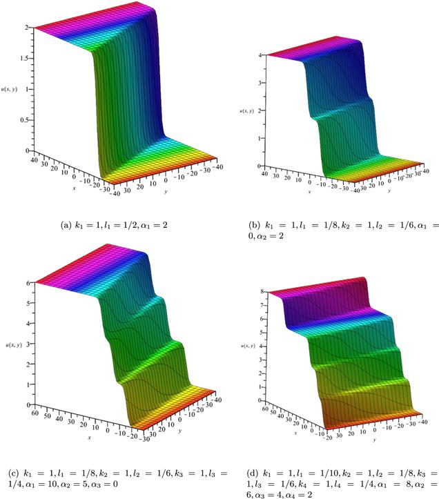
Figure 1. Multiple soliton wave when γ2 = 1/2, γ3 = −1, γ4 = 1/4, γ5 = 1/5, α = −1/5, t = 2. |
We now provide M-lump waves of the studied equation, using the long-wave method. Plugging ${{\rm{e}}}^{{\alpha }_{i}}=-1$ into equations (7 ), (3 ) holds the formula
$\begin{eqnarray*}{f}_{N}=\sum _{\mu =0,1}^{}\prod _{i=1}^{N}{\left(-1\right)}^{{\mu }_{i}}{{\rm{e}}}^{{\mu }_{i}{{\rm{\Phi }}}_{i}}\prod _{i\lt j}^{(N)}{{\rm{e}}}^{{\mu }_{i}{\mu }_{n}{A}_{{ij}}},\end{eqnarray*}$
where $\begin{eqnarray*}{{\rm{\Phi }}}_{i}={k}_{i}\left(x+{l}_{i}y-\left(\displaystyle \frac{{{k}_{i}}^{2}\alpha +{\gamma }_{2}+{l}_{i}\left({\gamma }_{4}+{l}_{i}{\gamma }_{5}\right)}{{\gamma }_{3}}\right)t\right)+{\alpha }_{i}.\end{eqnarray*}$
Inserting ki → 0 into fN, provides $\begin{eqnarray*}\begin{array}{l}f={f}_{N}=\displaystyle \sum _{\mu =0,1}^{}\displaystyle \prod _{i=1}^{N}{\left(-1\right)}^{{\mu }_{i}}\left(1+{\mu }_{i}{k}_{i}{{\rm{\Theta }}}_{i}\right)\\ \quad \times \displaystyle \prod _{i\lt j}^{(N)}(1+{\mu }_{i}{k}_{i}{\mu }_{j}{k}_{j}{B}_{{ij}})+O\left({k}^{N+1}\right).\end{array}\end{eqnarray*}$
It is obvious that $u=2\mathrm{ln}{\left({}^{{f}_{N}}/{}_{{\prod }_{i=1}^{N} \ \ {k}_{i}}\right)}_{x}$. To do more about the solution, the term ${\prod }_{i=1}^{N}{k}_{i}$ can be eliminated, and be replaced by fN. This leads us to $\begin{eqnarray*}\begin{array}{l}{f}_{N}=\displaystyle \prod _{i=1}^{N}{{\rm{\Theta }}}_{i}+\displaystyle \frac{1}{2}\displaystyle \sum _{i,j}^{(N)}{B}_{{ij}}\displaystyle \prod _{r\ne i,j}^{N}{{\rm{\Theta }}}_{r}+\cdots +\displaystyle \frac{1}{M!{2}^{M}}\\ \quad \times \displaystyle \sum _{i,j\cdots ,p,q}^{(N)}\mathop{\overbrace{{A}_{{ij}}{B}_{{kl}}\cdots {B}_{{pq}}}}\limits^{M}\displaystyle \prod _{s\ne i,j,k,l,\cdots ,p,q}^{N}{{\rm{\Theta }}}_{s}+\cdots ,\end{array}\end{eqnarray*}$
here, ${{\rm{\Theta }}}_{i}=x+{l}_{i}y-\left(\tfrac{{\gamma }_{2}+{l}_{i}\left({\gamma }_{4}+{l}_{i}{\gamma }_{5}\right)}{{\gamma }_{3}}\right)t$. ${\sum }_{i,j,\cdots ,p,q}^{N}$ is a collection of all feasible gatherings of i, j,...,p, q, that accept different values from 1, 2,...,N. If the parameters li affirm the situation ${l}_{M+i}={l}_{i}^{* }(i=1,2,...,M)$ with N = 2M and Bij > 0.Here we apply long-wave approach on equation (3 ) by considering N = 2, ki → 0, ${{\rm{e}}}^{{\alpha }_{i}}=-1\left(i=1,2\right)$ and $\tfrac{{k}_{1}}{{k}_{2}}=O\left(1\right)$, then equation (3 ) becomes7 ) could be rewritten as9 ) becomes13 )–(15 ) into (2 ), provides2 ) as shown in figure 2. This rational result is a permanent wave result decomposing as $O\left(\tfrac{1}{{x}^{2}},\tfrac{1}{{y}^{2}}\right)$ for $\left|x\right|,\left|y\right|\to \infty $ and travelling with the speed
$\begin{eqnarray}f={{\rm{\Theta }}}_{1}{{\rm{\Theta }}}_{2}+{B}_{12},\end{eqnarray}$
where equation ( $\begin{eqnarray}{{\rm{\Theta }}}_{i}=x+{l}_{i}y-\left(\displaystyle \frac{{\gamma }_{2}+{l}_{i}\left({\gamma }_{4}+{l}_{i}{\gamma }_{5}\right)}{{\gamma }_{3}}\right)t,\end{eqnarray}$
and equation ( $\begin{eqnarray}\begin{array}{l}{B}_{{ij}}=\displaystyle \frac{12\alpha }{{\left({l}_{i}-{l}_{j}\right)}^{2}{\gamma }_{5}},\,{l}_{\tfrac{N}{2}+i}={l}_{i}^{* },\left(i=1,2,..,\displaystyle \frac{N}{2}\right)\mathrm{and}\,i\lt j.\end{array}\end{eqnarray}$
Inserting equations ( $\begin{eqnarray}\begin{array}{rcl}u & = & 2\displaystyle \frac{\partial }{\partial x}\mathrm{log}\left({\left(x^{\prime} +{ay}^{\prime} \right)}^{2}+{b}^{2}y{{\prime} }^{2}-\displaystyle \frac{3\alpha }{{b}^{2}{\gamma }_{5}}\right)\\ & = & \displaystyle \frac{4\left(x^{\prime} +{ay}^{\prime} \right)}{{\left(x^{\prime} +{ay}^{\prime} \right)}^{2}+{b}^{2}y{{\prime} }^{2}-\tfrac{3\alpha }{{b}^{2}{\gamma }_{5}}}\end{array}\end{eqnarray}$
with $\begin{eqnarray*}x^{\prime} =x-\left(\displaystyle \frac{{\gamma }_{2}}{{\gamma }_{3}}-{a}^{2}\displaystyle \frac{{\gamma }_{5}}{{\gamma }_{3}}-{b}^{2}\displaystyle \frac{{\gamma }_{5}}{{\gamma }_{3}}\right)t.\end{eqnarray*}$
$\begin{eqnarray*}y^{\prime} =y-\left(\displaystyle \frac{{\gamma }_{4}}{{\gamma }_{3}}+2a\displaystyle \frac{{\gamma }_{5}}{{\gamma }_{3}}\right)t,\end{eqnarray*}$
With a single-M-lump wave for equation ( $\begin{eqnarray*}{v}_{x}=\displaystyle \frac{{\gamma }_{2}}{{\gamma }_{3}}-{a}^{2}\displaystyle \frac{{\gamma }_{5}}{{\gamma }_{3}}-{b}^{2}\displaystyle \frac{{\gamma }_{5}}{{\gamma }_{3}},\,\,\,\,\,\,\,\,\,\,{v}_{y}=\displaystyle \frac{{\gamma }_{4}}{{\gamma }_{3}}+2a\displaystyle \frac{{\gamma }_{5}}{{\gamma }_{3}}.\end{eqnarray*}$
Finding out that this wave travels in the following straight line is interesting $\begin{eqnarray*}y=\displaystyle \frac{\left({\gamma }_{4}+2{a}_{1}{\gamma }_{5}\right)\left(x+\sqrt{-\tfrac{3\alpha }{{{b}_{1}}^{2}{\gamma }_{5}}}\right)}{{\gamma }_{2}-\left({{a}_{1}}^{2}+{{b}_{1}}^{2}\right){\gamma }_{5}}.\end{eqnarray*}$
A one-M-lump wave that travels along this line at different times is drawn in figure 1(b).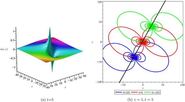
Figure 2. One-M-lump wave when a1 = 1/3, b1 = 8/7, γ2 = 1/2, γ3 = −1, γ4 = 1/4, γ5 = 1/5, α = −1/5. |
To derive a 2-M-lump result to equation (2 ), we let N = 4 in equation (3 ), and considering ${{\rm{e}}}^{{\alpha }_{i}}=-1\left(i=1,2,3,4\right)$, ki → 0, we provide14 ) and (15 ), respectively.
$\begin{eqnarray}\begin{array}{rcl}f & = & {{\rm{\Theta }}}_{1}{{\rm{\Theta }}}_{2}{{\rm{\Theta }}}_{3}{{\rm{\Theta }}}_{4}+{B}_{12}{{\rm{\Theta }}}_{3}{{\rm{\Theta }}}_{4}+{B}_{13}{{\rm{\Theta }}}_{2}{{\rm{\Theta }}}_{4}\\ & & +{B}_{14}{{\rm{\Theta }}}_{2}{{\rm{\Theta }}}_{3}+{B}_{23}{{\rm{\Theta }}}_{1}{{\rm{\Theta }}}_{4}\\ & & +{B}_{24}{{\rm{\Theta }}}_{1}{{\rm{\Theta }}}_{3}+{B}_{34}{{\rm{\Theta }}}_{1}{{\rm{\Theta }}}_{2}+{B}_{12}{{\rm{\Theta }}}_{34}\\ & & +{B}_{13}{{\rm{\Theta }}}_{24}+{B}_{14}{B}_{23},\end{array}\end{eqnarray}$
where Θ1, Θ2, Θ3, Θ4, wi, ${B}_{{ij}}\left(i\lt j\right)$ and ${l}_{\tfrac{N}{2}+i}$ are defined in equations (Inserting equations (17 ) into (3 ), provides
$\begin{eqnarray*}{y}_{1}=\displaystyle \frac{\left({\gamma }_{4}+2{a}_{1}{\gamma }_{5}\right)\left(x+\sqrt{-\tfrac{3\alpha }{{{b}_{1}}^{2}{\gamma }_{5}}}\right)}{{\gamma }_{2}-\left({{a}_{1}}^{2}+{{b}_{1}}^{2}\right){\gamma }_{5}},\end{eqnarray*}$
and $\begin{eqnarray*}{y}_{2}=\displaystyle \frac{\left({\gamma }_{4}+2{a}_{2}{\gamma }_{5}\right)\left(x+\sqrt{-\tfrac{3\alpha }{{{b}_{2}}^{2}{\gamma }_{5}}}\right)}{{\gamma }_{2}-\left({{a}_{2}}^{2}+{{b}_{2}}^{2}\right){\gamma }_{5}}.\end{eqnarray*}$
The travel of two-M-lump waves alongside the two lines is graphed in figure 3 in different periods.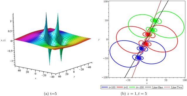
Figure 3. Two-M-lump wave when a1 = 1/3, b1 = 8/7, a2 = 1/4, b2 = 4/3, γ2 = 1/2, γ3 = −1, γ4 = 1/4, γ5 = 1/5, α = −1/5. |
To provide a 3M-lump result of equation (1 ), we implement ${k}_{i}\to 0,{{\rm{e}}}^{{\alpha }_{i}}=-1,\left(i=1,2,3,4,5,6\right)$ and consider N = 6 in equation (3 ), which provides14 ) and (15 ), respectively. Subsequently, inserting equations (21 ) into (3 ), a 3-M-lump result is provided as displayed in figure 4. We should know that l1 = a1 + ib1, l2 = a2 + ib2, l3 = a3 + ib3, ${l}_{4}={{l}_{1}}^{* }$, ${l}_{5}={{l}_{2}}^{* }$ and ${l}_{6}={{l}_{3}}^{* }$. The following straight lines are followed by a three-M-lump wave, which is interesting to know
$\begin{eqnarray}\begin{array}{rcl}{f}_{6} & = & {{\rm{\Theta }}}_{1}{{\rm{\Theta }}}_{2}{{\rm{\Theta }}}_{3}{{\rm{\Theta }}}_{4}{{\rm{\Theta }}}_{5}{{\rm{\Theta }}}_{6}+{B}_{12}{B}_{34}{B}_{56}\\ & & +{B}_{12}{B}_{35}{B}_{46}+{B}_{12}{B}_{45}{B}_{36}+{B}_{13}{B}_{24}{B}_{56}\\ & & +{B}_{13}{B}_{25}{B}_{46}+{B}_{13}{B}_{45}{B}_{26}\\ & & +{B}_{23}{B}_{14}{B}_{56}+{B}_{14}{B}_{25}{B}_{36}+{B}_{14}{B}_{35}{B}_{26}+{B}_{24}{B}_{15}{B}_{36}\\ & & +{B}_{34}{B}_{15}{B}_{26}+{B}_{23}{B}_{15}{B}_{46}+{B}_{23}{B}_{45}{B}_{16}\\ & & +{B}_{24}{B}_{35}{B}_{16}+{B}_{34}{B}_{25}{B}_{16}+{{\rm{\Theta }}}_{2}{{\rm{\Theta }}}_{3}{{\rm{\Theta }}}_{4}{{\rm{\Theta }}}_{5}{B}_{16}\\ & & +{{\rm{\Theta }}}_{2}{{\rm{\Theta }}}_{3}{{\rm{\Theta }}}_{5}{{\rm{\Theta }}}_{6}{B}_{14}\\ & & +{{\rm{\Theta }}}_{2}{{\rm{\Theta }}}_{3}{{\rm{\Theta }}}_{4}{{\rm{\Theta }}}_{6}{B}_{15}+{{\rm{\Theta }}}_{3}{{\rm{\Theta }}}_{4}{{\rm{\Theta }}}_{5}{{\rm{\Theta }}}_{6}{B}_{12}\\ & & +{{\rm{\Theta }}}_{2}{{\rm{\Theta }}}_{4}{{\rm{\Theta }}}_{5}{{\rm{\Theta }}}_{6}{B}_{13}+{{\rm{\Theta }}}_{1}{{\rm{\Theta }}}_{2}{{\rm{\Theta }}}_{4}{{\rm{\Theta }}}_{6}{B}_{35}+{{\rm{\Theta }}}_{1}{{\rm{\Theta }}}_{2}{{\rm{\Theta }}}_{4}{{\rm{\Theta }}}_{5}{B}_{36}\\ & & +{{\rm{\Theta }}}_{1}{{\rm{\Theta }}}_{4}{{\rm{\Theta }}}_{5}{{\rm{\Theta }}}_{6}{B}_{23}+{{\rm{\Theta }}}_{1}{{\rm{\Theta }}}_{3}{{\rm{\Theta }}}_{5}{{\rm{\Theta }}}_{6}{B}_{24}+{{\rm{\Theta }}}_{1}{{\rm{\Theta }}}_{3}{{\rm{\Theta }}}_{4}{{\rm{\Theta }}}_{6}{B}_{25}\\ & & +{{\rm{\Theta }}}_{1}{{\rm{\Theta }}}_{3}{{\rm{\Theta }}}_{4}{{\rm{\Theta }}}_{5}{B}_{26}+{{\rm{\Theta }}}_{1}{{\rm{\Theta }}}_{2}{{\rm{\Theta }}}_{3}{{\rm{\Theta }}}_{4}{B}_{56}+{{\rm{\Theta }}}_{1}{{\rm{\Theta }}}_{2}{{\rm{\Theta }}}_{3}{{\rm{\Theta }}}_{6}{B}_{45}\\ & & +{{\rm{\Theta }}}_{1}{{\rm{\Theta }}}_{2}{{\rm{\Theta }}}_{3}{{\rm{\Theta }}}_{5}{B}_{46}+{{\rm{\Theta }}}_{1}{{\rm{\Theta }}}_{2}{{\rm{\Theta }}}_{5}{{\rm{\Theta }}}_{6}{B}_{34}+{{\rm{\Theta }}}_{1}{{\rm{\Theta }}}_{2}{B}_{34}{B}_{56}\\ & & +{{\rm{\Theta }}}_{1}{{\rm{\Theta }}}_{2}{B}_{35}{B}_{46}+{{\rm{\Theta }}}_{1}{{\rm{\Theta }}}_{2}{B}_{45}{B}_{36}+{{\rm{\Theta }}}_{1}{B}_{23}{{\rm{\Theta }}}_{4}{B}_{56}\\ & & +{{\rm{\Theta }}}_{1}{B}_{23}{B}_{45}{{\rm{\Theta }}}_{6}+{{\rm{\Theta }}}_{1}{B}_{23}{{\rm{\Theta }}}_{5}{{B}_{4}}_{6}+{{\rm{\Theta }}}_{1}{{\rm{\Theta }}}_{3}{B}_{24}{B}_{56}\\ & & +{{\rm{\Theta }}}_{1}{{\rm{\Theta }}}_{6}{B}_{24}{B}_{35}+{{\rm{\Theta }}}_{1}{{\rm{\Theta }}}_{5}{B}_{24}{B}_{36}+{{\rm{\Theta }}}_{1}{{\rm{\Theta }}}_{3}{B}_{25}{B}_{46}\\ & & +{{\rm{\Theta }}}_{1}{{\rm{\Theta }}}_{6}{B}_{34}{B}_{25}+{{\rm{\Theta }}}_{1}{{\rm{\Theta }}}_{4}{B}_{25}{B}_{36}+{{\rm{\Theta }}}_{1}{{\rm{\Theta }}}_{3}{B}_{45}{B}_{26}\\ & & +{{\rm{\Theta }}}_{1}{{\rm{\Theta }}}_{5}{B}_{34}{B}_{26}+{{\rm{\Theta }}}_{1}{{\rm{\Theta }}}_{4}{B}_{35}{B}_{26}+{{\rm{\Theta }}}_{4}{{\rm{\Theta }}}_{5}{B}_{12}{B}_{36}\\ & & +{{\rm{\Theta }}}_{3}{{\rm{\Theta }}}_{4}{B}_{12}{B}_{56}+{{\rm{\Theta }}}_{3}{{\rm{\Theta }}}_{6}{B}_{12}{B}_{45}+{{\rm{\Theta }}}_{3}{{\rm{\Theta }}}_{5}{B}_{12}{B}_{46}\\ & & +{{\rm{\Theta }}}_{5}{{\rm{\Theta }}}_{6}{B}_{12}{B}_{34}+{{\rm{\Theta }}}_{4}{{\rm{\Theta }}}_{6}{B}_{12}{B}_{35}+{{\rm{\Theta }}}_{5}{{\rm{\Theta }}}_{6}{B}_{13}{B}_{24}\\ & & +{{\rm{\Theta }}}_{4}{{\rm{\Theta }}}_{6}{B}_{13}{B}_{25}+{{\rm{\Theta }}}_{4}{{\rm{\Theta }}}_{5}{B}_{13}{B}_{26}+{{\rm{\Theta }}}_{2}{{\rm{\Theta }}}_{4}{B}_{13}{B}_{56}\\ & & +{{\rm{\Theta }}}_{2}{{\rm{\Theta }}}_{6}{B}_{13}{B}_{45}+{{\rm{\Theta }}}_{2}{{\rm{\Theta }}}_{5}{B}_{13}{B}_{46}+{{\rm{\Theta }}}_{2}{{\rm{\Theta }}}_{3}{B}_{14}{B}_{56}\\ & & +{{\rm{\Theta }}}_{2}{{\rm{\Theta }}}_{6}{B}_{14}{B}_{35}+{{\rm{\Theta }}}_{2}{{\rm{\Theta }}}_{5}{B}_{14}{B}_{36}+{{\rm{\Theta }}}_{5}{{\rm{\Theta }}}_{6}{B}_{23}{B}_{14}\\ & & +{{\rm{\Theta }}}_{3}{{\rm{\Theta }}}_{6}{B}_{14}{B}_{25}+{{\rm{\Theta }}}_{3}{{\rm{\Theta }}}_{5}{B}_{14}{B}_{26}+{{\rm{\Theta }}}_{4}{{\rm{\Theta }}}_{6}{B}_{23}{B}_{15}\\ & & +{{\rm{\Theta }}}_{3}{{\rm{\Theta }}}_{6}{B}_{24}{B}_{15}+{{\rm{\Theta }}}_{3}{{\rm{\Theta }}}_{4}{B}_{15}{B}_{26}+{{\rm{\Theta }}}_{2}{{\rm{\Theta }}}_{3}{B}_{15}{B}_{46}\\ & & +{{\rm{\Theta }}}_{2}{{\rm{\Theta }}}_{6}{B}_{34}{B}_{15}+{{\rm{\Theta }}}_{2}{{\rm{\Theta }}}_{4}{B}_{15}{B}_{36}\\ & & +{{\rm{\Theta }}}_{2}{{\rm{\Theta }}}_{4}{B}_{35}{B}_{16}+{{\rm{\Theta }}}_{4}{{\rm{\Theta }}}_{5}{B}_{23}{B}_{16}\\ & & +{{\rm{\Theta }}}_{3}{{\rm{\Theta }}}_{5}{B}_{24}{B}_{16}+{{\rm{\Theta }}}_{3}{{\rm{\Theta }}}_{4}{B}_{25}{B}_{16}\\ & & +{{\rm{\Theta }}}_{2}{{\rm{\Theta }}}_{3}{B}_{45}{B}_{16}+{{\rm{\Theta }}}_{2}{{\rm{\Theta }}}_{5}{B}_{34}{B}_{16}.\end{array}\end{eqnarray}$
We should know that Θ1, Θ2, Θ3, Θ4, Θ5, Θ6, Bij and ${l}_{\tfrac{N}{2}+i}$ are provides in equations ( $\begin{eqnarray*}{y}_{1}=\displaystyle \frac{\left({\gamma }_{4}+2{a}_{1}{\gamma }_{5}\right)\left(x+\sqrt{-\tfrac{3\alpha }{{{b}_{1}}^{2}{\gamma }_{5}}}\right)}{{\gamma }_{2}-\left({{a}_{1}}^{2}+{{b}_{1}}^{2}\right){\gamma }_{5}},\end{eqnarray*}$
$\begin{eqnarray*}{y}_{2}=\displaystyle \frac{\left({\gamma }_{4}+2{a}_{2}{\gamma }_{5}\right)\left(x+\sqrt{-\tfrac{3\alpha }{{{b}_{2}}^{2}{\gamma }_{5}}}\right)}{{\gamma }_{2}-\left({{a}_{2}}^{2}+{{b}_{2}}^{2}\right){\gamma }_{5}},\end{eqnarray*}$
and $\begin{eqnarray*}{y}_{3}=\displaystyle \frac{\left({\gamma }_{4}+2{a}_{3}{\gamma }_{5}\right)\left(x+\sqrt{-\tfrac{3\alpha }{{{b}_{3}}^{2}{\gamma }_{5}}}\right)}{{\gamma }_{2}-\left({{a}_{3}}^{2}+{{b}_{3}}^{2}\right){\gamma }_{5}}.\end{eqnarray*}$
In figure 5, the three-M-lump waves' path along these three lines is graphed for various times.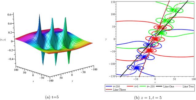
Figure 4. Three-M-lump wave when a1 = 1/3, b1 = 8/7, a2 = 1/4, b2 = 9/7, a3 = 1/5, b3 = 10/7, γ2 = 1/2, γ3 = −1, γ4 = 1/4, γ5 = 1/5, α = −1/5. |
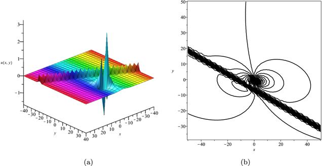
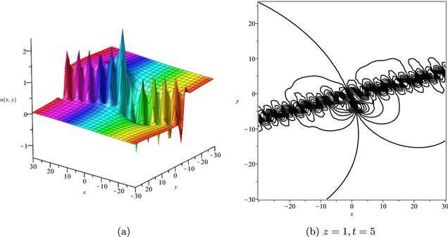
Figure 5. Mixed M-lump-soliton wave when a1 = 1/3, b1 = 3/2, k3 = 1, l3 = 2, α3 = 5, γ2 = 1/2, γ3 = −1, γ4 = 1/4, γ5 = 1/5, α = −1/5, t = 5. |
3. Collision phenomena
This section attempts to design the collision of a 1-M-lump result along with one-soliton, two-soliton, and a 2-M-lump wave with a single soliton. To begin with, we set N = 3 in equation (3 ) and take the limit ${k}_{i}\to 0,\left(i=1,2\right)$ and $\tfrac{{k}_{1}}{{k}_{2}}=O\left(1\right)$, and this provides7 ), ${{\rm{\Theta }}}_{i}\left(i=1,2\right)$ are provided in equation (14 ), B12 is given in equation (15 ). C13, C23 are derived as follows20 ) into (19 ), and then into equation (3 ), as shown in figure 4.
$\begin{eqnarray}f={{\rm{\Theta }}}_{1}{{\rm{\Theta }}}_{2}+{B}_{12}+{\xi }_{1}{{\rm{e}}}^{{{\rm{\Phi }}}_{3}},\end{eqnarray}$
where $\begin{eqnarray*}{\xi }_{1}={{\rm{\Theta }}}_{1}{{\rm{\Theta }}}_{2}+{B}_{12}+{C}_{23}{{\rm{\Theta }}}_{1}+{C}_{13}{{\rm{\Theta }}}_{2}+{C}_{13}{C}_{23}.\end{eqnarray*}$
Here Φ3 is expressed in equation ( $\begin{eqnarray}{C}_{{ij}}=-\displaystyle \frac{12{k}_{j}\alpha }{3{{k}_{j}}^{2}\alpha -{\left({l}_{i}-{l}_{j}\right)}^{2}{\gamma }_{5}}\,\,\,\,\,\,\,\,\,\,i\lt j.\end{eqnarray}$
A result that depicts the interaction between a 1-M-lump solution and a 1-soliton solution is obtained by putting equations (To provide a collision of two-soliton with an M-lump wave, we consider that14 ) and (20 ). The functions Φi and Θi are provided in equations (7 ) and (15 ). Inserting equations (21 ) into (2 ), an outcome is a result that stands for a collision between a one-M-lump wave and a two-soliton solution which display in figure 6.
$\begin{eqnarray}\begin{array}{l}f={B}_{12}+{\xi }_{1}{{\rm{e}}}^{{{\rm{\Phi }}}_{3}}+{\xi }_{2}{{\rm{e}}}^{{{\rm{\Phi }}}_{4}}+{{\rm{\Theta }}}_{1}{{\rm{\Theta }}}_{2}-{{\rm{e}}}^{{{\rm{\Phi }}}_{3}+{{\rm{\Phi }}}_{4}+{A}_{34}}\\ \quad \times \left({{\rm{\Theta }}}_{1}{{\rm{\Theta }}}_{2}+{B}_{12}-{C}_{14}{C}_{23}-{C}_{13}{C}_{24}-{\xi }_{1}-{\xi }_{2}\right),\end{array}\end{eqnarray}$
where $\begin{eqnarray*}{\xi }_{1}={{\rm{\Theta }}}_{1}{{\rm{\Theta }}}_{2}+{B}_{12}+{C}_{23}{{\rm{\Theta }}}_{1}+{C}_{13}{{\rm{\Theta }}}_{2}+{C}_{13}{C}_{23},\end{eqnarray*}$
and $\begin{eqnarray*}{\xi }_{2}={{\rm{\Theta }}}_{1}{{\rm{\Theta }}}_{2}+{B}_{12}+{C}_{24}{{\rm{\Theta }}}_{1}+{C}_{14}{{\rm{\Theta }}}_{2}+{C}_{14}{C}_{24}.\end{eqnarray*}$
The constants Bij and Cij are provided in equations (
Figure 6. Mixed M-lump-two-soliton wave when a1 = 1/3, b1 = 3/2, a2 = 1/4, b2 = 9/7, k3 = 1, l3 = 2, k4 = 3/4, l4 = 1, α3 = 10, α4 = 0, γ2 = 1/2, γ3 = −1, γ4 = 1/4, γ5 = 1/5, α = −1/5, t = 5. |
When N = 5 and considering the limit ${k}_{i}\to 0,\left(i=1,2,3,4\right)$ in equation (3 ), the collision between two-M-lump wave and one-soliton are22 ) into (3 ), and the consequence is the aspect displayed in figure 7.
$\begin{eqnarray}\begin{array}{rcl}f & = & {{\rm{\Theta }}}_{1}{{\rm{\Theta }}}_{2}{{\rm{\Theta }}}_{3}{{\rm{\Theta }}}_{4}+{B}_{34}{{\rm{\Theta }}}_{1}{{\rm{\Theta }}}_{2}+{B}_{24}{{\rm{\Theta }}}_{1}{{\rm{\Theta }}}_{3}\\ & & +{B}_{23}{{\rm{\Theta }}}_{1}{{\rm{\Theta }}}_{4}+{B}_{14}{{\rm{\Theta }}}_{2}{{\rm{\Theta }}}_{3}+{B}_{13}{{\rm{\Theta }}}_{2}{{\rm{\Theta }}}_{4}\\ & & +{B}_{12}{{\rm{\Theta }}}_{3}{{\rm{\Theta }}}_{4}+Q{{\rm{e}}}^{{k}_{5}\left(x+{l}_{5}y+{w}_{5}t\right)+{\alpha }_{5}}\\ & & +{B}_{14}{B}_{23}+{B}_{13}{B}_{24}+{B}_{12}{B}_{34},\end{array}\end{eqnarray}$
where $\begin{eqnarray*}\begin{array}{rcl}Q & = & {{\rm{\Theta }}}_{1}{{\rm{\Theta }}}_{2}{{\rm{\Theta }}}_{3}{{\rm{\Theta }}}_{4}+{C}_{45}{{\rm{\Theta }}}_{1}{{\rm{\Theta }}}_{2}{{\rm{\Theta }}}_{3}+{C}_{15}{{\rm{\Theta }}}_{2}{{\rm{\Theta }}}_{3}{{\rm{\Theta }}}_{4}\\ & & +{C}_{25}{{\rm{\Theta }}}_{1}{{\rm{\Theta }}}_{3}{{\rm{\Theta }}}_{4}\\ & & +{C}_{35}{{\rm{\Theta }}}_{1}{{\rm{\Theta }}}_{2}{{\rm{\Theta }}}_{4}+\left({B}_{34}+{C}_{35}{C}_{45}\right){{\rm{\Theta }}}_{1}{{\rm{\Theta }}}_{2}\\ & & +\left({B}_{24}+{C}_{25}{C}_{45}\right){{\rm{\Theta }}}_{1}{{\rm{\Theta }}}_{3}+\left({B}_{14}+{C}_{15}{C}_{45}\right){{\rm{\Theta }}}_{2}{{\rm{\Theta }}}_{3}\\ & & +\left({B}_{23}+{C}_{25}{C}_{35}\right){{\rm{\Theta }}}_{1}{{\rm{\Theta }}}_{4}+\left({B}_{13}+{C}_{15}{C}_{35}\right){{\rm{\Theta }}}_{2}{{\rm{\Theta }}}_{4}\\ & & +\left({B}_{12}+{C}_{15}{C}_{25}\right){{\rm{\Theta }}}_{3}{{\rm{\Theta }}}_{4}+\left({B}_{34}{C}_{25}+{B}_{24}{C}_{35}\right.\\ & & \left.+{B}_{23}{C}_{45}+{C}_{25}{C}_{35}{C}_{45}\right){{\rm{\Theta }}}_{1}\\ & & +\left({B}_{34}{C}_{15}+{B}_{14}{C}_{35}+{B}_{13}{C}_{45}+{C}_{15}{C}_{35}{C}_{45}\right){{\rm{\Theta }}}_{2}\\ & & +\left({B}_{24}{C}_{15}+{B}_{14}{C}_{25}+{B}_{12}{C}_{45}+{C}_{15}{C}_{25}{C}_{45}\right){{\rm{\Theta }}}_{3}\\ & & +\left({B}_{23}{C}_{15}+{B}_{13}{C}_{25}+{B}_{12}{C}_{35}+{C}_{15}{C}_{25}{C}_{35}\right){{\rm{\Theta }}}_{4}\\ & & +{B}_{14}{B}_{23}+{B}_{13}{B}_{24}+{B}_{12}{B}_{34}+{B}_{34}{C}_{15}{C}_{25}\\ & & +{B}_{24}{C}_{15}{C}_{35}+{B}_{14}{C}_{25}{C}_{35}\\ & & +{B}_{23}{C}_{15}{C}_{45}+{B}_{13}{C}_{25}{C}_{45}\\ & & +{B}_{12}{C}_{35}{C}_{45}+{C}_{15}{C}_{25}{C}_{35}{C}_{45}.\end{array}\end{eqnarray*}$
In this article, all constants and functions are listed. Now that we have provided a collision between a two-M-lump and a one-soliton solution, inserting equations (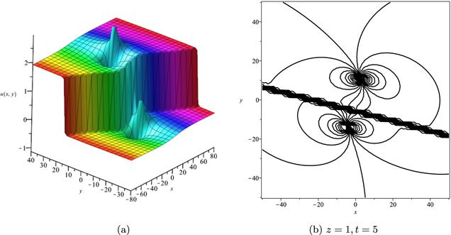
Figure 7. Mixed two-M-lump-soliton wave when a1 = 1/3, b1 = 8/7, a2 = 1/4, b2 = 4/3, k5 = 1, l5 = 4, α5 = 1, γ2 = 1/2, γ3 = −1, γ4 = 1/4, γ5 = 1/5, α = −1/5, t = 5. |
4. Breather solution and its interactions
In this section, we try to explore some new solutions to the suggested equation like breather wave, mixed breather-soliton, and mixed breather-M-lump waves. Taking ${k}_{1}=\tfrac{1}{4}+{\rm{i}},{{\rm{k}}}_{2}={{k}_{1}}^{* },{l}_{1}=\tfrac{1}{2}+{\rm{i}}$, ${l}_{2}={{l}_{1}}^{* }$ in equation (10 ) then into equation (2 ) a result yields a breather wave as presented in figure 8.
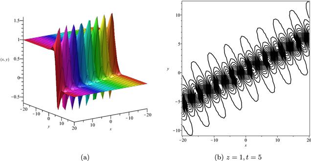
Figure 8. Breather wave when α1 = 0, α2 = 0, γ2 = 1/2, γ3 = −1, γ4 = 1/4, γ52 = 1/5, α = −1/5, t = 2. |
An interaction physical phenomena between breather and soliton solution could be constructed by taking ${k}_{1}=\tfrac{1}{4}+{\rm{i}},{{\rm{k}}}_{2}={{k}_{1}}^{* },{l}_{1}=\tfrac{1}{2}+{\rm{i}},\,{l}_{2}={{l}_{1}}^{* }$ in equation (12 ) then substituting these values into equation (2 ), an outcome gives us a mixed breather-soliton wave as seen in figure 9.
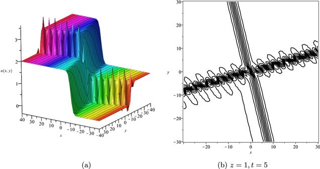
Figure 9. Mixed breather-soliton wave when k3 = 1, l3 = 1/4, α1 = 0, α2 = 0, α3 = 0, γ2 = 1/2, γ3 = −1, γ4 = 1/4, γ52 = 1/5, α = −1/5, t = 2. |
Moreover, to offer a mixed breather-M-lump wave, we let N = 4, ${k}_{3}=\tfrac{1}{5}+{\rm{i}},{{\rm{k}}}_{4}={{k}_{3}}^{* },{l}_{3}=\tfrac{1}{2}+{\rm{i}},\,{l}_{4}={{l}_{3}}^{* }$ in equation (21 ) and putting these values into equation (2 ) gives an interaction between the breather wave and M-lump wave as shown in figure 10.
Figure 10. Mixed breather-M-lump wave when a1 = 1/3, b1 = 10/7, a2 = 1/4, b2 = 13/7, α3 = 0, α4 = 0, γ2 = 1/2, γ3 = −1, γ4 = 1/4, γ52 = 1/5, α = −1/5, t = 2. |
5. Conclusions
This study investigated the generalized Hietarintatype equation. Multiple M-lump waves alongside their collision phenomena to multiple M-lump waves with soliton wave solutions are auspiciously provided. Using suitable values of parameter, we put out the physical features of the reported results through three dimensional and contour graphics. The results presented express physical features of lump and lump interaction phenomena of different kinds of nonlinear physical processes. Further, Breather solutions and their interactions such as breather waves, mixed breather-solitons, and mixed breather-M-lump waves have been investigated. In a subsequent paper, we analyze the extended Hietarintatype equation with variable coefficients and derive a number of novel conclusions for this model.
Conflict of interest
The authors declare that they have no conflict of interest.
Ethical standard
The author state that this research paper complies with ethical standards. This research paper does not involve either human participants or animals.