Welcome to visit Communications in Theoretical Physics,
Mathematical Physics

Higher-order rogue waves with controllable fission and asymmetry localized in a (3 + 1)-dimensional generalized Boussinesq equation

  • Sheng Zhang , * ,
  • Ying Li
Expand
  • School of Mathematical Sciences, Bohai University, Jinzhou, China

*Author to whom any correspondence should be addressed.

Received date: 2022-07-14

  Revised date: 2022-10-11

  Accepted date: 2022-10-14

  Online published: 2022-12-22

Copyright

© 2022 Institute of Theoretical Physics CAS, Chinese Physical Society and IOP Publishing

Abstract

The purpose of this paper is to report the feasibility of constructing high-order rogue waves with controllable fission and asymmetry for high-dimensional nonlinear evolution equations. Such a nonlinear model considered in this paper as the concrete example is the (3 + 1)-dimensional generalized Boussinesq (gB) equation, and the corresponding method is Zhaqilao's symbolic computation approach containing two embedded parameters. It is indicated by the (3 + 1)-dimensional gB equation that the embedded parameters can not only control the center of the first-order rogue wave, but also control the number of the wave peaks split from higher-order rogue waves and the asymmetry of higher-order rogue waves about the coordinate axes. The main novelty of this paper is that the obtained results and findings can provide useful supplements to the method used and the controllability of higher-order rogue waves.

Cite this article

Sheng Zhang , Ying Li . Higher-order rogue waves with controllable fission and asymmetry localized in a (3 + 1)-dimensional generalized Boussinesq equation[J]. Communications in Theoretical Physics, 2023 , 75(1) : 015003 . DOI: 10.1088/1572-9494/ac9a3e

1. Introduction

Rogue waves were originally used to describe the extremely destructive water waves on the ocean, which appeared from nowhere and disappeared without a trace [1]. From the point of view of mathematics, rogue waves are a kind of special non-singular rational solutions of nonlinear evolution equations. In 1965, the concept of ‘freak rogue waves' was first proposed by Draper [2]. Since then, the study of rogue waves has attracted widespread attention like those [319] and some effective methods have been proposed for constructing rogue wave solutions, such as Darboux transformation [4, 6, 7], Hirota's bilinear method [8, 9], inverse scattering transform [10, 11] and so on. To be more specific, Solli, Ropers, Koonath and Jalali [3] reported the rogue waves observed by them in the optical system and modelled the generation of these rogue waves through the generalized nonlinear Schrödinger (NLS) equation; Akhmediev, Ankiewicz and Soto-Crespo [4] presented a modified Darboux scheme for constructing rogue wave solutions of the standard self-focusing NLS equation; Yan [5] gave the term ‘financial rogue waves' based on the nonlinear option equation; Guo, Ling and Liu [7] proposed the generalized Darboux transformation to construct Nth-order rogue wave solutions of physically interested models and illustrated its feasibility with two concrete examples; Ohta and Yang [8] derived Nth-order rogue wave solutions of the NLS equation by Hirota's bilinear method; Randoux, Suret and El [10] used a local periodization procedure to give inverse scattering transform analysis of rogue wave solutions of the NLS equation; Ma [16] presented the polynomial conjecture related to rogue waves in the Korteweg-de Vries equation.
More recently, some researchers [2027] have focused on studying rogue wave solutions, especially higher-order rogue wave solutions of (3 + 1)-dimensional nonlinear models. In 2018, Zhaqilao [22] proposed the so-called symbolic computation approach to constructing rogue wave solutions with controllable centers of two high-dimensional nonlinear systems. Compared with the other methods [4, 8, 10], the symbolic computation approach [22] is direct and does not depend on the τ-function and Lax pair analysis which require high skills. More importantly, a pair of parameters embedded in the method [22] has been proven to be able to control the centers of rogue waves in terms of position and quantity. It is worth mentioning that the method [22] without these two parameters is only its initial version [21]. In this paper, we find that in addition to controlling the center of a first-order rogue wave, these two parameters can also control the fission and asymmetry of higher-order rogue waves. However, the findings on fission and asymmetry of higher-order rogue waves are not reported in [22]. Since the high asymmetry is another prominent feature of rogue waves besides steepness and instantaneity, it is of great significance to construct asymmetric rogue waves. Although there are a few studies on asymmetric rogue waves, such as [2830], these studies either stay on the image display or have no substantive discussion on the regularity of control factors. In this article, we shall use the method [22] to construct higher-order rogue wave solutions with controllable fission and asymmetry of the following (3 + 1)-dimensional generalized Boussinesq (gB) equation [27]:
$\begin{eqnarray}{u}_{tt}+\alpha {({u}^{2})}_{xx}+\beta {u}_{xxxx}+\gamma {u}_{xx}-{u}_{yy}-{u}_{zz}=0,\end{eqnarray}$
where $\alpha ,$ $\beta $ and $\gamma $ are constants, and the influence laws of two parameters controlling the fission and asymmetry of higher-order rogue wave solutions are discussed. In 2019, Yan [27] bilinearized equation (1) and obtained its two-soliton solutions based on Bell polynomial theory. Meanwhile, Yan [27] also obtained a breather wave solution and first-order rogue wave solution of equation (1) by using the extended homoclinic test method. As far as we know, the higher-order rogue wave solution of equation (1) and its fission and asymmetry has not been reported.
We arrange the rest of this paper as follows: section 2 describes Zhaqilao's symbolic computation approach [22]; section 3 gives the Painlevé analysis and bilinear form of equation (1); in section 4, the first-, second-, third- and fourth-order rogue wave solutions of equation (1) are constructed by the method [22], and then the effects of the two parameters included in the constructed rogue wave solutions on the center, fission and asymmetry of the rogue waves are discussed; and section 5 concludes this paper and discusses the potential physical applications of the results obtained.

2. Description of Zhaqilao's symbolic computation approach

To construct rogue wave solutions of the (3 + 1)-dimensional gB equation (1), we first recall Zhaqilao's symbolic computation approach [22]. For a given (3 + 1)-dimensional nonlinear partial differential equation (PDE) assumed as:
$\begin{eqnarray}P(u,{u}_{x},{u}_{y},{u}_{z},{u}_{t},{u}_{xx},{u}_{xy},{u}_{xz},{u}_{xt},\cdot \cdot \cdot )=0,\end{eqnarray}$
where $P$ is usually a polynomial of $u$ and its various partial derivatives with respect to $x,$ $y,$ $z$ and $t,$ or any other expression which can be transformed into such a polynomial, we outline the steps of the method [22] as follows:

Based on the Painlevé analysis, we take a transformation:

$\begin{eqnarray}u=T(f),\end{eqnarray}$
where f is an undetermined function of the independent variables $x,$ $y,$ $z$ and $t;$

With the help of equation (3), we assume that equation (2) can be transformed into the following Hirota's bilinear form:

$\begin{eqnarray}R({D}_{\xi },{D}_{z};f)=0,\,\xi =x+ay-ct,\end{eqnarray}$
where $a$ and $c$ are undetermined real constants, ${D}_{\xi }$ and ${D}_{z}$ are Hirota's operators [31]:
$\begin{eqnarray}\begin{array}{l}{D}_{\xi }^{m}{D}_{z}^{n}f(\xi ,z)\cdot g(\xi ,z)={({\partial }_{\xi }-{\partial }_{\xi ^{\prime} })}^{m}{({\partial }_{z}-{\partial }_{z^{\prime} })}^{n}\\ \,\times f(\xi ,z)g(\xi ^{\prime} ,z^{\prime} ){| }_{\xi =\xi ^{\prime} ,z=z^{\prime} },\,(m,n\in N);\end{array}\end{eqnarray}$

We suppose that

$\begin{eqnarray}\begin{array}{l}f={\tilde{F}}_{n+1}(\xi ,z;\theta ,\vartheta )={F}_{n+1}(\xi ,z,a)+2\theta z{F}_{n}(\xi ,z,b)\\ \,+2\vartheta \xi {F}_{n}(\xi ,z,c)+({\theta }^{2}+{\vartheta }^{2}){F}_{n-1}(\xi ,z,a),\end{array}\end{eqnarray}$
where
$\begin{eqnarray}\begin{array}{l}{F}_{n}(\xi ,z,\varepsilon )=\displaystyle \sum _{k=0}^{n(n+1)/2}\displaystyle \sum _{i=0}^{k}{\varepsilon }_{n(n+1)-2k,2i}{z}^{2i}{\xi }^{n(n+1)-2k},\,\\ (\varepsilon =a,b,c),\end{array}\end{eqnarray}$
with the initial values
$\begin{eqnarray}{F}_{-1}(\xi ,z,a)={F}_{0}(\xi ,z,b)={F}_{0}(\xi ,z,c)=0,\end{eqnarray}$
while ${a}_{j,l},$ ${b}_{j,l}$ and ${c}_{j,l}(j,l\in \{0,2,4,\cdot \cdot \cdot ,n(n+1)\})$ are all real undetermined constants, $\theta $ and $\vartheta $ are two embedded parameters in the rogue wave solutions to be constructed.

Substituting equation (6) into equation (4), and then setting all the coefficients of the same powers of ${z}^{p}{\xi }^{q}(p,q=0,1,2,\cdot \cdot \cdot )$ to be zeros, we can derive a system of polynomial equations for ${a}_{j,l},$ ${b}_{j,l}$ and ${c}_{j,l}(j,l\,\in \{0,2,4,\cdot \cdot \cdot ,n(n+1)\}).$

Solving the system of polynomial equations derived above and substituting the obtained values of ${a}_{j,l},$ ${b}_{j,l}$ and ${c}_{j,l}(j,l\in \{0,2,4,\cdot \cdot \cdot ,n(n+1)\})$ into equation (7), we get some rational solutions of equation (2) by means of equations (3) and (6), and from which the first-, second- and other higher-order rogue wave solutions localized in $\xi $ and $z$ can be obtained.

3. Painlevé analysis and bilinear form

By Painlevé analysis, the following auto-Bäcklund transformation for the (3 + 1)-dimensional gB equation (1) can be derived:

$\begin{eqnarray}u=\displaystyle \frac{6\beta }{\alpha }{(\mathrm{ln}\,\phi )}_{xx}+{u}_{0},\end{eqnarray}$
where ${u}_{0}$ is a solution of equation (1), while the real function $\phi $ of $x,$ $y,$ $z$ and $t$ satisfies the system of nonlinear PDEs:
$\begin{eqnarray}{\phi }_{t}^{2}-{\phi }_{y}^{2}-{\phi }_{z}^{2}+(\gamma +2\alpha {u}_{0}){\phi }_{x}^{2}-3\beta {\phi }_{xx}^{2}+4\beta {\phi }_{x}{\phi }_{xxx}=0,\end{eqnarray}$
$\begin{eqnarray}\begin{array}{l}{\phi }_{x}^{2}({\phi }_{tt}-{\phi }_{yy}-{\phi }_{zz}+6\gamma {\phi }_{xx}+9\beta {\phi }_{xxxx})\\ \,+\,{\phi }_{xx}({\phi }_{t}^{2}-{\phi }_{y}^{2}-{\phi }_{z}^{2}-3\beta {\phi }_{xx}^{2})\\ \,+\,2{\phi }_{x}[{({\phi }_{t}^{2}-{\phi }_{y}^{2}-{\phi }_{z}^{2})}_{x}+4\alpha {u}_{0}{\phi }_{x}^{3}]=0,\end{array}\end{eqnarray}$
$\begin{eqnarray}\begin{array}{l}{\phi }_{{xx}}\left({\phi }_{{tt}}-{\phi }_{{yy}}-{\phi }_{{zz}}\right)-2\beta {\phi }_{{xxx}}^{2}+3\beta {\phi }_{{xx}}{\phi }_{{xxxx}}\\ \,+\,2\left({\phi }_{{xt}}^{2}-{\phi }_{{xy}}^{2}-{\phi }_{{xz}}^{2}\right)\\ \,+\,2\alpha {u}_{0,{xx}}{\phi }_{x}^{2}+2{\phi }_{x}\left[{\left({\phi }_{{tt}}-{\phi }_{{yy}}-{\phi }_{{zz}}\right)}_{x}+6\alpha {u}_{0,x}{\phi }_{{xx}}^{2}\right.\\ \,+\,\left.2\left(\gamma +2\alpha {u}_{0}\right){\phi }_{{xxx}}+3\beta {\phi }_{{xxxxx}}\right]=0.\end{array}\end{eqnarray}$

Firstly, we suppose that

$\begin{eqnarray}u=\displaystyle \sum _{j=0}^{\infty }{v}_{j}{\phi }^{j-n},\,({v}_{0}\ne 0),\end{eqnarray}$
where ${v}_{j}(j=0,1,2,\cdot \cdot \cdot )$ are real functions of $x,$ $y,$ $z$ and $t$ to be determined later.
Secondly, substituting equation (13) into equation (1) and analyzing the leading terms of $\alpha {({u}^{2})}_{xx}$ and $\beta {u}_{xxxx}$ yields
$\begin{eqnarray}-2n-2=-n-4,\end{eqnarray}$
$\begin{eqnarray}2\alpha n(2n+1){v}_{0}^{2}{\phi }_{x}^{2}+\beta n(n+1)(n+2)(n+3){v}_{0}{\phi }_{x}^{4}=0,\end{eqnarray}$
which hint
$\begin{eqnarray}n=2,\,{v}_{0}=-\displaystyle \frac{6\beta }{\alpha }{\phi }_{x}^{2}.\end{eqnarray}$
Further letting
$\begin{eqnarray}{v}_{j}=0(j\geqslant 3),\,{v}_{2}={u}_{0},\end{eqnarray}$
and inserting equations (13), (16) and (17) into equation (1), then setting all the coefficients of the same powers of ${\phi }^{s}(s=-5,-4,-3,-2,-1,0)$ to be zeros, we have
$\begin{eqnarray}{v}_{1}=\displaystyle \frac{6\beta }{\alpha }{\phi }_{xx},\end{eqnarray}$
$\begin{eqnarray}{v}_{2,tt}+\alpha {({v}_{2}^{2})}_{xx}+\beta {v}_{2,xxxx}+\gamma {v}_{2,xx}-{v}_{2,yy}-{v}_{2,zz}=0,\end{eqnarray}$
besides equations (10)–(12).
With the help of equations (13) and (16)–(18) we finally reach equation (9). It is easy to see from equations (17) and (19) that ${v}_{2}$ or ${u}_{0}$ is a solution of equation (1).

The (3 + 1)-dimensional gB equation (1) has the following Hirota's bilinear form:

$\begin{eqnarray}(\omega {D}_{\xi }^{2}+\beta {D}_{\xi }^{4}-{D}_{z}^{2})f\cdot f=0,\end{eqnarray}$
where $f$ is a real function of $\xi $ and $z,$ and $\omega $ and $\xi $ always represent
$\begin{eqnarray}\omega =-{a}^{2}+{c}^{2}+\gamma ,\end{eqnarray}$
$\begin{eqnarray}\xi =x+ay-ct,\end{eqnarray}$
where $a$ and $c$ are two real constants.

Obviously, equations (21) and (22) can reduce equation (1) as:

$\begin{eqnarray}\omega {u}_{\xi \xi }+3{({u}^{2})}_{\xi \xi }+\beta {u}_{\xi \xi \xi \xi }-{u}_{zz}=0.\end{eqnarray}$
We next introduce
$\begin{eqnarray}u={u}_{0}+{q}_{\xi \xi },\end{eqnarray}$
here u0 is assumed as a constant. Equation (1) can be written as
$\begin{eqnarray}\omega {q}_{\xi \xi }+\alpha {({u}_{0}+{q}_{\xi \xi })}^{2}+\beta {q}_{\xi \xi \xi \xi }-{q}_{zz}=0\end{eqnarray}$
by integrating the resulting equation derived from the substitution of equation (24) into equation (1) with respect to $\xi $ twice and selecting the two integration constants as zeros.
In view of equations (9) and (24), we assume that
$\begin{eqnarray}q=\displaystyle \frac{6\beta }{\alpha }\,\mathrm{ln}\,f,\end{eqnarray}$
and substitute equation (26) into equation (25), then the following equivalent equation is derived:
$\begin{eqnarray}\begin{array}{l}\omega ({f}_{\xi \xi }f-{{f}_{\xi }}^{2})-({f}_{zz}f-{{f}_{z}}^{2})+\beta ({f}_{\xi \xi \xi \xi }f-4{f}_{\xi \xi \xi }{f}_{\xi }+3{{f}_{\xi \xi }}^{2})\\ \,=\,0,\end{array}\end{eqnarray}$
if and only if ${u}_{0}=0.$ We finally transform equation (27) into equation (20) by Hirota's operators (5).

4. Rogue wave solutions

Based on the bilinear form (27), we construct the first-, second-, three- and four-order rogue wave solutions of the (3 + 1)-dimensional gB equation (1).

4.1. First-order rogue wave solution

For the first-order rogue wave solution, we consider the case of $n=0$ in equation (6) and select
$\begin{eqnarray}f={F}_{1}(\xi ,z,a)={a}_{2,0}{\xi }^{2}+{a}_{0,2}{z}^{2}+{a}_{0,0}.\end{eqnarray}$
Substituting equation (28) into equation (27) and setting all the coefficients of the same powers of ${z}^{p}{\xi }^{q}(p,q\,=0,1,2,\cdot \cdot \cdot )$ to be zeros, we get a set of polynomial equations for ${a}_{2,0},$ ${a}_{0,2}$ and ${a}_{0,0}.$ Solving the polynomial equations, we have
$\begin{eqnarray}{a}_{2,0}=1,\,{a}_{0,2}=-\omega ,\,{a}_{0,0}=-\displaystyle \frac{3\beta }{\omega },\end{eqnarray}$
and then obtain the first-order rogue wave solution of equation (1):
$\begin{eqnarray}u=-\displaystyle \frac{12\omega \beta [3\beta +\omega {(\xi -\theta )}^{2}+{\omega }^{2}{(z-\vartheta )}^{2}]}{\alpha {[3\beta -\omega {(\xi -\theta )}^{2}+{\omega }^{2}{\left(z-\vartheta \right)}^{2}]}^{2}}.\end{eqnarray}$
Here a pair of parameters $\theta $ and $\vartheta $ have been embedded into equation (28) so that $f$ can be taken the following form:
$\begin{eqnarray}f={\tilde{F}}_{1}(\xi ,z;\theta ,\vartheta )={a}_{2,0}{(\xi -\theta )}^{2}+{a}_{0,2}{(z-\vartheta )}^{2}+{a}_{0,0},\end{eqnarray}$
which ensures that equation (30) still solves equation (1). This is due to equations (28) and (31) having the same partial derivatives with respect to $\xi $ and $z.$
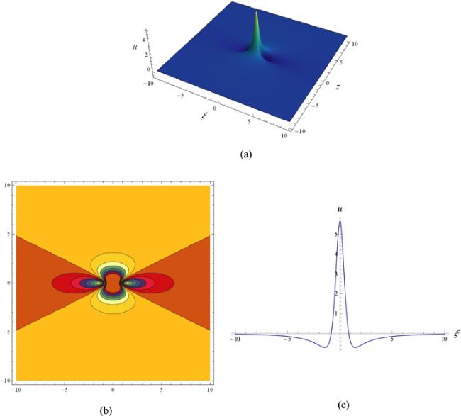
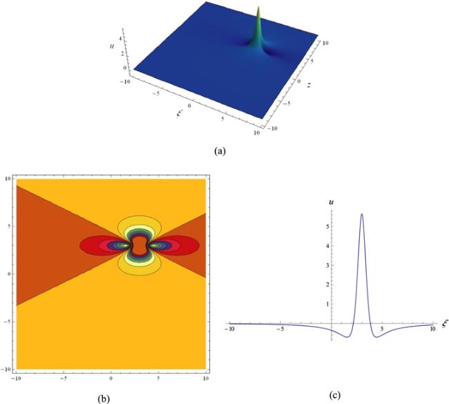
In figure 1, the first-order rogue wave solution (30) is shown by setting
$\begin{eqnarray}a=-4.6,\,c=-3.15,\,\alpha =3,\,\beta =1,\,\gamma =7,\end{eqnarray}$
and $\theta =\vartheta =0,$ respectively. At the same time, except for different $\theta =\vartheta =3,$ the selection of other parameters is the same as that in figure 1, we use figure 2 to show the first-order rogue wave solution (30). As can be seen from figures 1 and 2, the first-order rogue wave is symmetric about the lines $\xi =0$ and $z=0,$ and its center is controlled by the parameters $\theta $ and $\vartheta .$ Specifically, when $\theta =\vartheta =0,$ the first-order rogue wave has the extreme value at the location $(0,0),$ but for different $\theta =\vartheta =3,$ the extreme value appears at the point $(3,3).$
Figure 1. First-order rogue wave localized in (30) with $a=-4.6,$ $c=-3.15,$ $\alpha =3,$ $\beta =1,$ $\gamma =7,$ $\vartheta =0$ and $\theta =0,$ (a) 3D graph; (b) contour plot; (c) profile at $z=0.$
Figure 2. First-order rogue wave localized in (30) with $a=-4.6,$ $c=-3.15,$ $\alpha =3,$ $\beta =1,$ $\gamma =7,$ $\vartheta =3$ and $\theta =3,$ (a) 3D graph; (b) contour plot; (c) profile at $z=3.$

4.2. Second-order rogue wave solution

For the second-order rogue wave solution, we consider equation (6) when $n=1,$ that is
$\begin{eqnarray}\begin{array}{l}f={\tilde{F}}_{2}(\xi ,z;\theta ,\vartheta )={F}_{2}(\xi ,z,a)+2\theta z{F}_{1}(\xi ,z,b)\\ \,+\,2\vartheta \xi {F}_{1}(\xi ,z,c)+{\theta }^{2}+{\vartheta }^{2},\end{array}\end{eqnarray}$
where
$\begin{eqnarray}\begin{array}{l}{F}_{2}(\xi ,z,a)=({a}_{4,2}{z}^{2}+{a}_{4,0}){\xi }^{4}+({a}_{2,4}{z}^{4}+{a}_{2,2}{z}^{2}){\xi }^{2}\\ \,+\,{a}_{0,6}{z}^{6}+{a}_{0,4}{z}^{4}+{a}_{6,0}+{F}_{1}(\xi ,z,a),\end{array}\end{eqnarray}$
and ${F}_{1}(\xi ,z,a),$ ${F}_{1}(\xi ,z,b)$ and ${F}_{1}(\xi ,z,c)$ are determined by:
$\begin{eqnarray}{F}_{1}(\xi ,z,\varepsilon )={\varepsilon }_{2,0}{\xi }^{2}+{\varepsilon }_{0,2}{z}^{2}+{\varepsilon }_{0,0},\,(\varepsilon =a,b,c).\end{eqnarray}$
Substituting equation (33) into equation (27) and setting all the coefficients of the same powers of ${z}^{p}{\xi }^{q}(p,q=0,1,2,\cdot \cdot \cdot )$ to be zeros, we get a set of polynomial equations for ${a}_{6,0},$ ${a}_{4,2},$ ${a}_{4,0},$ ${a}_{2,4},$ ${a}_{2,2},$ ${a}_{2,0},$ ${a}_{0,6},$ ${a}_{0,4},$ ${a}_{0,2},$ ${a}_{0,0},$ ${b}_{2,0},$ ${b}_{0,2},$ ${b}_{0,0},$ ${c}_{2,0},$ ${c}_{0,2}$ and ${c}_{0,0}.$ Solving the polynomial equations, we gain
$\begin{eqnarray}\begin{array}{l}{a}_{6,0}=1,\,{a}_{4,2}=-3\omega ,\,{a}_{4,0}=-\displaystyle \frac{25\beta }{\omega },\,{a}_{2,4}=3{\omega }^{2},\\ {a}_{2,2}=90\beta ,\,{a}_{2,0}=-\displaystyle \frac{125{\beta }^{2}}{{\omega }^{2}},\end{array}\end{eqnarray}$
$\begin{eqnarray}\begin{array}{l}{a}_{0,6}=-{\omega }^{3},\,{a}_{0,4}=-17\beta \omega ,\,{a}_{0,2}=-\displaystyle \frac{475{\beta }^{2}}{\omega },\\ {a}_{0,0}=-\displaystyle \frac{16875{\beta }^{3}+{\omega }^{2}{\theta }^{2}+9{\omega }^{3}{\theta }^{2}}{9{\omega }^{3}},\end{array}\end{eqnarray}$
$\begin{eqnarray}\begin{array}{l}{b}_{2,0}=1,\,{b}_{0,2}=\displaystyle \frac{\omega }{3},\,{b}_{0,0}=-\displaystyle \frac{5\beta }{3\omega },\,{c}_{2,0}=1,\,{c}_{0,2}=3\omega ,\\ {c}_{0,0}=\displaystyle \frac{\beta }{\omega },\end{array}\end{eqnarray}$
and therefore obtain the second-order rogue wave solution of equation (1):
$\begin{eqnarray}u=\displaystyle \frac{6\beta }{\alpha }{(\mathrm{ln}\,{\tilde{F}}_{2}(\xi ,z;\theta ,\vartheta ))}_{\xi \xi },\end{eqnarray}$
where ${\tilde{F}}_{2}(\xi ,z;\theta ,\vartheta )$ is determined by equations (33)–(38).
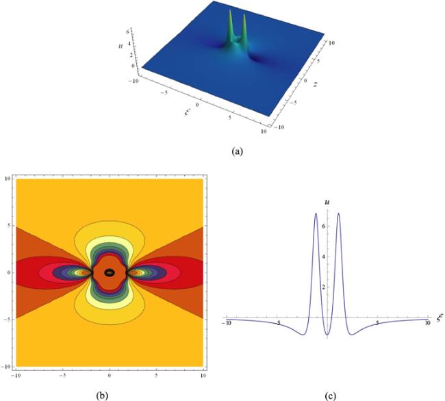
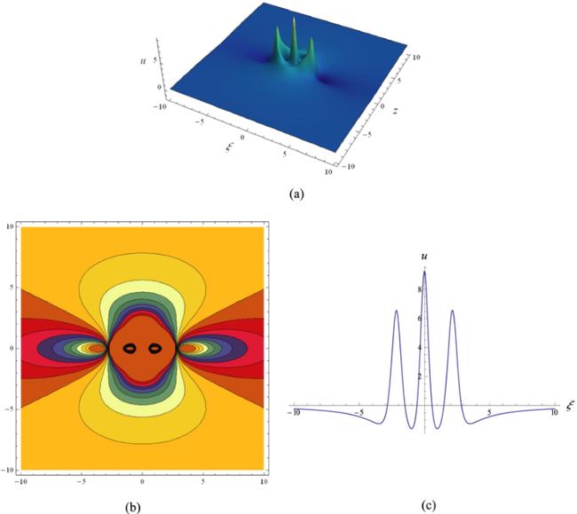
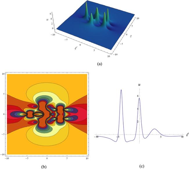
In figures 3 and 4, we show the second-order rogue wave solution (39). It can be seen from figure 3 that when $\theta =\vartheta =0$ the second-order rogue wave has two interaction wave peaks. However, with the increase of $\theta $ and $\vartheta ,$ the computer simulation shows that these two interaction wave peaks gradually separate and give birth to the third wave peak. For the case of $\theta =\vartheta =200,$ figure 4 shows the second-order rogue wave with three separated wave peaks. In addition, we can see that the second-order rogue wave in figure 3 is symmetric with respect to the lines $\xi =0$ and $z=0,$ but the one in figure 4 is asymmetric.
Figure 3. Second-order rogue wave localized in (39) with $a=-4.6,$ $c=-3.15,$ $\alpha =3,$ $\beta =1,$ $\gamma =7,$ $\vartheta =0$ and $\theta =0,$ (a) 3D graph; (b) contour plot; (c) profile at $z=0.$
Figure 4. Second-order rogue wave localized in (39) with $a=-4.6,$ $c=-3.15,$ $\alpha =3,$ $\beta =1,$ $\gamma =7,$ $\theta =200$ and $\vartheta =200,$ (a) 3D graph; (b) contour plot; (c) profile at $z=2.$

4.3. Third-order rogue wave solution

For the third-order rogue wave solution, we consider equation (6) with $n=2:$
$\begin{eqnarray}\begin{array}{l}f={\tilde{F}}_{3}(\xi ,z;\theta ,\vartheta )={F}_{3}(\xi ,z,a)+2\theta z{F}_{2}(\xi ,z,b)\\ \,+\,2\vartheta \xi {F}_{2}(\xi ,z,c)+({\theta }^{2}+{\vartheta }^{2}){F}_{1}(\xi ,z,a),\end{array}\end{eqnarray}$
where
$\begin{eqnarray}\begin{array}{l}{F}_{3}(\xi ,z,a)={a}_{12,0}{\xi }^{12}+({a}_{10,2}{z}^{2}+{a}_{10,0}){\xi }^{10}\\ \,+\,({a}_{8,4}{z}^{4}+{a}_{8,2}{z}^{2}+{a}_{8,0}){\xi }^{8}\\ \,+\,({a}_{6,6}{z}^{6}+{a}_{6,4}{z}^{4}+{a}_{6,2}{z}^{2}){\xi }^{6}\\ \,+\,({a}_{4,8}{z}^{8}+{a}_{4,6}{z}^{6}+{a}_{4,4}{z}^{4}){\xi }^{4}\\ \,+\,({a}_{2,10}{z}^{10}+{a}_{2,8}{z}^{8}+{a}_{2,6}{z}^{6}){\xi }^{2}+{a}_{0,12}{z}^{12}+{a}_{0,10}{z}^{10}\\ \,+{a}_{0,8}{z}^{8}+{F}_{2}(\xi ,z,a),\end{array}\end{eqnarray}$
and ${F}_{2}(\xi ,z,a),$ ${F}_{2}(\xi ,z,b)$ and ${F}_{2}(\xi ,z,c)$ are determined by:
$\begin{eqnarray}\begin{array}{l}{F}_{2}(\xi ,z,\varepsilon )=({\varepsilon }_{4,2}{z}^{2}+{\varepsilon }_{4,0}){\xi }^{4}+({\varepsilon }_{2,4}{z}^{4}+{\varepsilon }_{2,2}{z}^{2}){\xi }^{2}\\ \,+{\varepsilon }_{0,6}{z}^{6}+{\varepsilon }_{0,4}{z}^{4}+{\varepsilon }_{6,0}+{F}_{1}(\xi ,z,\varepsilon ),\,(\varepsilon =a,b,c),\end{array}\end{eqnarray}$
respectively.
Substituting equation (40) into equation (27) and setting all the coefficients of the same powers of ${z}^{p}{\xi }^{q}(p,q=0,1,2,\cdot \cdot \cdot )$to be zeros, we get a set of polynomial equations for the undetermined constants in equations (35), (41) and (42), from which we have
$\begin{eqnarray}\begin{array}{l}{a}_{12,0}=1,\,{a}_{10,2}=-6\omega ,\,{a}_{10,0}=-\displaystyle \frac{98\beta }{\omega },\,{a}_{8,4}=15{\omega }^{2},\\ {a}_{8,2}=690\beta ,\,{a}_{8,0}=\displaystyle \frac{735{\beta }^{2}}{{\omega }^{2}},\end{array}\end{eqnarray}$
$\begin{eqnarray}\begin{array}{l}{a}_{6,6}=-20{\omega }^{3},\,{a}_{6,4}=-1540\omega \beta ,\,{a}_{6,2}=-\displaystyle \frac{18620{\beta }^{2}}{\omega },\\ {a}_{6,0}=-\displaystyle \frac{75460{\beta }^{3}}{3{\omega }^{3}},\,{a}_{4,8}=15{\omega }^{4},\end{array}\end{eqnarray}$
$\begin{eqnarray}\begin{array}{l}{a}_{4,6}=1460{\omega }^{2}\beta ,\,{a}_{4,4}=37450{\beta }^{2},\,{a}_{4,2}=\displaystyle \frac{220500{\beta }^{3}}{{\omega }^{2}},\\ {a}_{4,0}=-\displaystyle \frac{5187875{\beta }^{4}}{3{\omega }^{4}},\end{array}\end{eqnarray}$
$\begin{eqnarray}\begin{array}{l}{a}_{2,10}=-6{\omega }^{5},\,{a}_{2,8}=-570{\omega }^{3}\beta ,\,{a}_{2,6}=-35420\omega {\beta }^{2},\\ {a}_{2,4}=\displaystyle \frac{14700{\beta }^{3}}{\omega },\end{array}\end{eqnarray}$
$\begin{eqnarray}\begin{array}{l}{a}_{2,2}=-\displaystyle \frac{565950{\beta }^{4}}{{\omega }^{3}},\,\\ {a}_{2,0}=-\displaystyle \frac{3994663750{\beta }^{5}+3{\omega }^{4}{\theta }^{2}-75{\omega }^{5}{\vartheta }^{2}}{75{\omega }^{5}(1+{\theta }^{2}+{\vartheta }^{2})},\\ {a}_{0,12}={\omega }^{6},\end{array}\end{eqnarray}$
$\begin{eqnarray}\begin{array}{l}{a}_{0,10}=58{\omega }^{4}\beta ,\,{a}_{0,8}=4335{\omega }^{2}{\beta }^{2},\,{a}_{0,6}=\displaystyle \frac{798980{\beta }^{3}}{3},\\ {a}_{0,4}=\displaystyle \frac{16391725{\beta }^{4}}{3{\omega }^{2}},\end{array}\end{eqnarray}$
$\begin{eqnarray}{a}_{0,2}=\displaystyle \frac{7522418750{\beta }^{5}+3{\omega }^{4}{\theta }^{2}-75{\omega }^{5}{\vartheta }^{2}}{75{\omega }^{4}(1+{\theta }^{2}+{\vartheta }^{2})},\end{eqnarray}$
$\begin{eqnarray}\begin{array}{l}{a}_{0,0}=\displaystyle \frac{21970650625{\beta }^{6}+27{\omega }^{4}\beta {\theta }^{2}-675{\omega }^{5}\beta {\vartheta }^{2}}{225{\omega }^{6}(1+{\theta }^{2}+{\vartheta }^{2})},\,\\ {b}_{6,0}=1,\,{b}_{4,2}=\omega ,\,{b}_{4,0}=-\displaystyle \frac{21\beta }{\omega },\end{array}\end{eqnarray}$
$\begin{eqnarray}\begin{array}{l}{b}_{2,4}=-\displaystyle \frac{9{\omega }^{2}}{5},\,{b}_{2,2}=-38\beta ,\,{b}_{2,0}=-\displaystyle \frac{133{\beta }^{2}}{{\omega }^{2}},\\ {b}_{0,6}=-\displaystyle \frac{{\omega }^{3}}{5},\end{array}\end{eqnarray}$
$\begin{eqnarray}\begin{array}{l}{b}_{0,4}=\displaystyle \frac{7\omega \beta }{5},\,{b}_{0,2}=\displaystyle \frac{49{\beta }^{2}}{\omega },\,{b}_{0,0}=-\displaystyle \frac{3773{\beta }^{3}}{3{\omega }^{3}},\,{c}_{6,0}=1,\\ {c}_{4,2}=9\omega ,\end{array}\end{eqnarray}$
$\begin{eqnarray}\begin{array}{l}{c}_{4,0}=-\displaystyle \frac{13\beta }{\omega },\,{c}_{2,4}=-5{\omega }^{2},\,{c}_{2,2}=-230\beta ,\,\\ {c}_{2,0}=-\displaystyle \frac{245{\beta }^{2}}{{\omega }^{2}},\end{array}\end{eqnarray}$
$\begin{eqnarray}\begin{array}{l}{c}_{0,6}=-5{\omega }^{3},\,{c}_{0,4}=-45\omega \beta ,\,{c}_{0,2}=-\displaystyle \frac{535{\beta }^{2}}{\omega },\\ {c}_{0,0}=-\displaystyle \frac{12005{\beta }^{3}}{3{\omega }^{3}}\end{array}\end{eqnarray}$
and therefore obtain the third-order rogue wave solution of equation (1):
$\begin{eqnarray}u=2{(\mathrm{ln}\,{\tilde{F}}_{3}(\xi ,z;\theta ,\vartheta ))}_{\xi \xi },\end{eqnarray}$
where ${\tilde{F}}_{3}(\xi ,z;\theta ,\vartheta )$ is determined by equations (40)–(54).
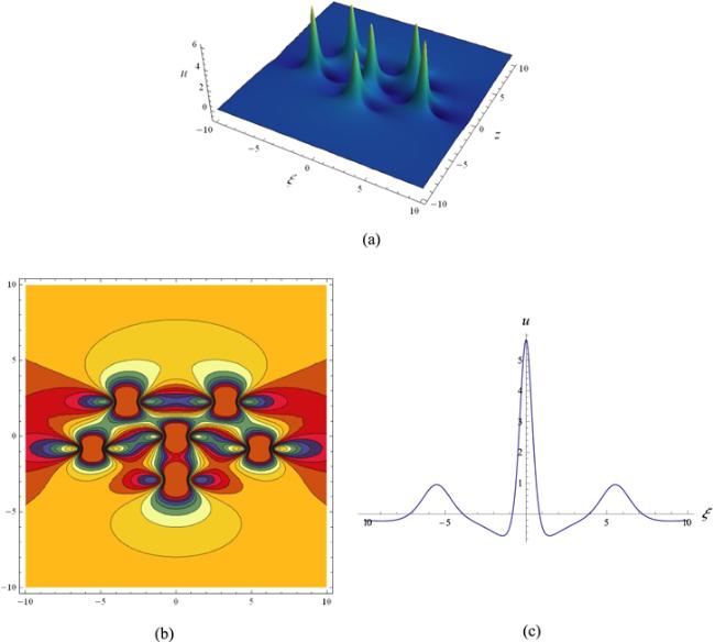
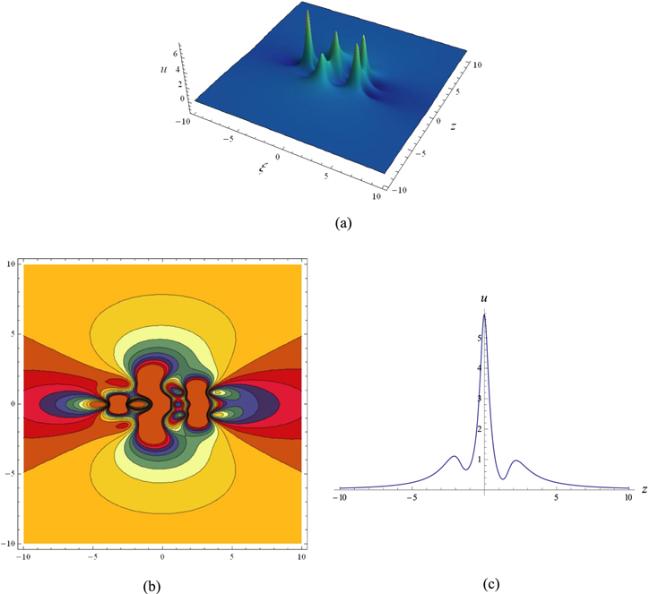
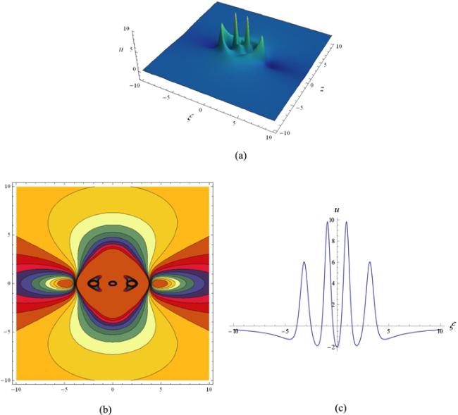
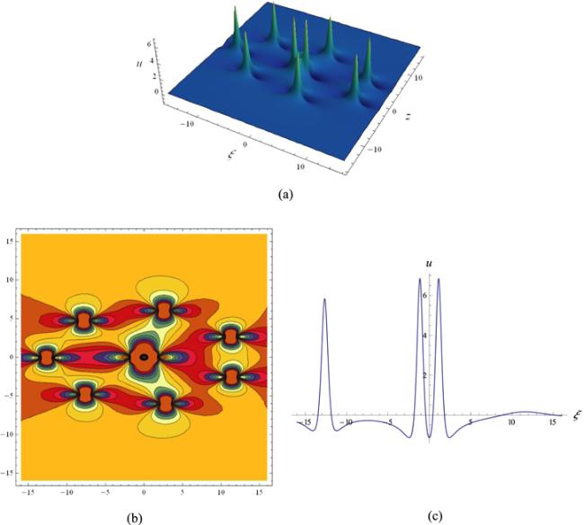
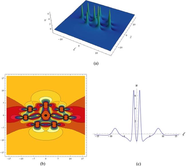
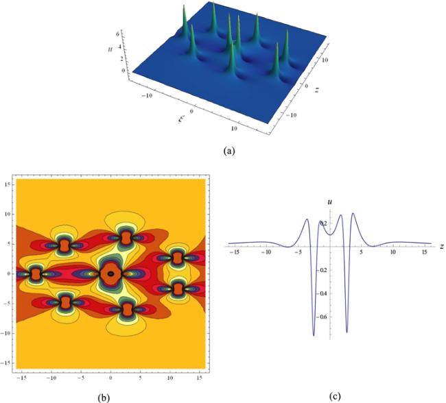
In figure 5, we show the third-order rogue wave solution (55) with three interaction wave peaks, which is symmetric with respect to the lines $\xi =0$ and $z=0.$ The highest wave peak is located at the center $(0,0),$ and the other two entangled second highest wave peaks surround the center. Similar to the second-order rogue wave in figure 3, the three interaction wave peaks in figure 5 gradually separate and give birth to another three wave peaks as long as one or all of $\theta $ and $\vartheta $ is/are given sufficiently large value(s). When either $\theta $ or $\vartheta $ is equal to zero, we show the third-order rogue wave solution (55) that is symmetric with respect to the lines $\xi =0$ and $z=0$ in figures 6 and 7, respectively. That is to say that $\theta =0$ makes the third-order rogue wave symmetric with respect to the line $\xi =0,$ while $\vartheta =0$ makes the third-order rogue wave symmetric with respect to the line $z=0.$ However, for the non-zeros $\theta $ and $\vartheta ,$ the third-order rogue wave is asymmetric, see figure 8 for example.
Figure 5. Third-order rogue wave localized in (55) with $a=-4.6,$ $c=-3.15,$ $\alpha =3,$ $\beta =1,$ $\gamma =7,$ $\theta =0$ and $\vartheta =0,$ (a) 3D graph; (b) contour plot; (c) profile at $z=0.$
Figure 6. Third-order rogue wave localized in (55) with $a=-4.6,$ $c=-3.15,$ $\alpha =3,$ $\beta =1,$ $\gamma =7,$ $\theta =0$ and $\vartheta =2000,$ (a) 3D graph; (b) contour plot; (c) profile plot at $z=0.$
Figure 7. Third-order rogue wave localized in (55) with $a=-4.6,$ $c=-3.15,$ $\alpha =3,$ $\beta =1,$ $\gamma =7,$ $\theta =0$ and $\vartheta =9\times {10}^{4},$ (a) 3D graph; (b) contour plot; (c) profile at $z=0.$
Figure 8. Third-order rogue wave localized in (55) with $a=-4.6,$ $c=-3.15,$ $\alpha =3,$ $\beta =1,$ $\gamma =7,$ $\theta =600$ and $\vartheta =600,$ (a) 3D graph; (b) contour plot; (c) profile at $\xi =0.$

4.4. Fourth-order rogue wave solutions

For the fourth-order rogue wave solution, we consider equation (6) with $n=3:$
$\begin{eqnarray}\begin{array}{l}f={\tilde{F}}_{4}(\xi ,z;\theta ,\vartheta )={F}_{4}(\xi ,z,a)+2\theta z{F}_{3}(\xi ,z,b)\\ \,+\,2\vartheta \xi {F}_{3}(\xi ,z,c)+({\theta }^{2}+{\vartheta }^{2}){F}_{2}(\xi ,z,a),\end{array}\end{eqnarray}$
where
$\begin{eqnarray}\begin{array}{l}{F}_{4}(\xi ,z,a)={a}_{20,0}{\xi }^{20}+({a}_{18,2}{z}^{2}+{a}_{18,0}){\xi }^{18}\\ \,+\,({a}_{16,4}{z}^{4}+{a}_{16,2}{z}^{2}+{a}_{16,0}){\xi }^{16}\\ \,+\,({a}_{14,6}{z}^{6}+{a}_{14,4}{z}^{4}+{a}_{14,2}{z}^{2}+{a}_{14,0}){\xi }^{14}\\ \,+\,({a}_{12,8}{z}^{8}+{a}_{12,6}{z}^{6}+{a}_{12,4}{z}^{4}+{a}_{12,2}{z}^{2}+{a}_{12,0}){\xi }^{12}\\ \,+\,({a}_{10,10}{z}^{10}+{a}_{10,8}{z}^{8}+{a}_{10,6}{z}^{6}+{a}_{10,4}{z}^{4}){\xi }^{10}\\ \,+\,({a}_{8,12}{z}^{12}+{a}_{8,10}{z}^{10}+{a}_{8,8}{z}^{8}+{a}_{8,6}{z}^{6}){\xi }^{8}\\ \,+\,({a}_{6,14}{z}^{14}+{a}_{6,12}{z}^{12}+{a}_{6,10}{z}^{10}+{a}_{6,8}{z}^{8}){\xi }^{6}\\ \,+\,({a}_{4,16}{z}^{16}+{a}_{4,14}{z}^{14}+{a}_{4,12}{z}^{12}+{a}_{4,10}{z}^{10}){\xi }^{4}\\ \,+\,({a}_{2,18}{z}^{18}+{a}_{2,16}{z}^{16}+{a}_{2,14}{z}^{14}+{a}_{2,12}{z}^{12}){\xi }^{2}\\ \,+\,{a}_{0,20}{z}^{20}+{a}_{0,18}{z}^{18}+{a}_{0,16}{z}^{16}+{a}_{0,14}{z}^{14}+{F}_{3}(\xi ,z,a),\end{array}\end{eqnarray}$
and ${F}_{3}(\xi ,z,a),$ ${F}_{3}(\xi ,z,b)$ and ${F}_{3}(\xi ,z,c)$ are determined by:
$\begin{eqnarray}\begin{array}{l}{F}_{3}(\xi ,z,\varepsilon )={\varepsilon }_{12,0}{\xi }^{12}+({\varepsilon }_{10,2}{z}^{2}+{\varepsilon }_{10,0}){\xi }^{10}\\ \,+\,({\varepsilon }_{8,4}{z}^{4}+{\varepsilon }_{8,2}{z}^{2}+{\varepsilon }_{8,0}){\xi }^{8}\\ \,+\,({\varepsilon }_{6,6}{z}^{6}+{\varepsilon }_{6,4}{z}^{4}+{\varepsilon }_{6,2}{z}^{2}){\xi }^{6}\\ \,+\,({\varepsilon }_{4,8}{z}^{8}+{\varepsilon }_{4,6}{z}^{6}+{\varepsilon }_{4,4}{z}^{4}){\xi }^{4}\\ \,+\,({\varepsilon }_{2,10}{z}^{10}+{\varepsilon }_{2,8}{z}^{8}+{\varepsilon }_{2,6}{z}^{6}){\xi }^{2}+{\varepsilon }_{0,12}{z}^{12}+{\varepsilon }_{0,10}{z}^{10}\\ \,+\,{\varepsilon }_{0,8}{z}^{8}+{F}_{2}(\xi ,z,\varepsilon ),\,(\varepsilon =a,b,c),\end{array}\end{eqnarray}$
respectively.
Substituting equation (56) into equation (27) and setting all the coefficients of the same powers of ${z}^{p}{\xi }^{q}(p,q=0,1,2,\cdot \cdot \cdot )$ to be zeros, we get a set of polynomial equations, and from which the undetermined constants can be determined as follows:
$\begin{eqnarray}\begin{array}{l}{a}_{20,0}=1,\,{a}_{18,2}=-10\omega ,\,{a}_{18,0}=-\displaystyle \frac{270}{\omega },\,{a}_{16,4}=45{\omega }^{2},\\ {a}_{16,2}=3030\beta ,\end{array}\end{eqnarray}$
$\begin{eqnarray}\begin{array}{l}{a}_{16,0}=\displaystyle \frac{16605{\beta }^{2}}{{\omega }^{2}},\,{a}_{14,6}=-120{\omega }^{3},\,{a}_{14,4}=-13800\omega \beta ,\\ {a}_{14,2}=-\displaystyle \frac{275400{\beta }^{2}}{\omega },\end{array}\end{eqnarray}$
$\begin{eqnarray}\begin{array}{l}{a}_{14,0}=-\displaystyle \frac{351000{\beta }^{3}}{{\omega }^{3}},\,{a}_{12,8}=210{\omega }^{4},\,{a}_{12,6}=34440{\omega }^{2}\beta ,\\ {a}_{12,4}=1367100{\beta }^{2},\end{array}\end{eqnarray}$
$\begin{eqnarray}\begin{array}{l}{a}_{12,2}=\displaystyle \frac{10621800{\beta }^{3}}{{\omega }^{2}},\,{a}_{12,0}=-\displaystyle \frac{18877950{\beta }^{4}}{{\omega }^{4}},\\ {a}_{10,10}=-252{\omega }^{5},{a}_{10,8}=-52500{\omega }^{3}\beta ,\end{array}\end{eqnarray}$
$\begin{eqnarray}\begin{array}{l}{a}_{10,6}=-3308760\omega {\beta }^{2},\,{a}_{10,4}=-\displaystyle \frac{56586600{\beta }^{3}}{\omega },\\ {a}_{10,2}=-\displaystyle \frac{107534700{\beta }^{4}}{{\omega }^{3}},\end{array}\end{eqnarray}$
$\begin{eqnarray}\begin{array}{l}{a}_{10,0}=-\displaystyle \frac{2094264900{\beta }^{5}}{{\omega }^{5}},{a}_{8,12}=210{\omega }^{6},\\ {a}_{8,10}=50820{\omega }^{4}\beta ,\,{a}_{8,8}=4513950{\omega }^{2}{\beta }^{2},\end{array}\end{eqnarray}$
$\begin{eqnarray}\begin{array}{l}{a}_{8,6}=135286200{\beta }^{3},\,{a}_{8,4}=\displaystyle \frac{1071960750{\beta }^{4}}{{\omega }^{2}},\\ {a}_{8,2}=\displaystyle \frac{4871002500{\beta }^{6}}{{\omega }^{4}},\end{array}\end{eqnarray}$
$\begin{eqnarray}\begin{array}{l}{a}_{8,0}=-\displaystyle \frac{178095030750}{{\omega }^{6}},{a}_{6,14}=-120{\omega }^{7},\\ {a}_{6,12}=-31080{\omega }^{5}\beta ,{a}_{6,10}=-3601080{\omega }^{3},\end{array}\end{eqnarray}$
$\begin{eqnarray}\begin{array}{l}{a}_{6,8}=-151237800\omega {\beta }^{3},{a}_{6,6}=-\displaystyle \frac{3824793000{\beta }^{4}}{\omega },\\ {a}_{6,4}=-\displaystyle \frac{636363000{\beta }^{5}}{{\omega }^{3}}\end{array}\end{eqnarray}$
$\begin{eqnarray}\begin{array}{l}{a}_{6,2}=\displaystyle \frac{521628471000{\beta }^{6}}{{\omega }^{5}},\,\\ {a}_{6,0}=\displaystyle \frac{341392530943000{\beta }^{7}+{\theta }^{2}{\omega }^{6}-49{\vartheta }^{2}{\omega }^{7}}{49{\omega }^{7}(1+{\theta }^{2}+{\vartheta }^{2})},\end{array}\end{eqnarray}$
$\begin{eqnarray}\begin{array}{l}{a}_{4,16}=45{\omega }^{8},\,{a}_{4,14}=11400{\omega }^{6}\beta ,\,{a}_{4,12}=1619100{\omega }^{4}{\beta }^{2},\\ {a}_{4,10}=94613400{\omega }^{2}{\beta }^{3},\end{array}\end{eqnarray}$
$\begin{eqnarray}\begin{array}{l}{a}_{4,8}=2667498750{\beta }^{4},\,{a}_{4,6}=\displaystyle \frac{45237339000{\beta }^{5}}{{\omega }^{2}},\\ {a}_{4,4}=-\displaystyle \frac{405853402500{\beta }^{6}}{{\omega }^{4}},\end{array}\end{eqnarray}$
$\begin{eqnarray}{a}_{4,2}=\displaystyle \frac{1631039216625000{\beta }^{7}+3{\omega }^{6}{\theta }^{2}-147{\omega }^{7}{\vartheta }^{2}}{49{\omega }^{6}(1+{\theta }^{2}+{\vartheta }^{2})},\end{eqnarray}$
$\begin{eqnarray}{a}_{4,0}=\displaystyle \frac{9338356860958125{\beta }^{8}+25\beta {\omega }^{6}{\theta }^{2}-1225\beta {\omega }^{7}{\vartheta }^{2}}{49{\omega }^{8}(1+{\theta }^{2}+{\vartheta }^{2})},\end{eqnarray}$
$\begin{eqnarray}\begin{array}{l}{a}_{2,18}=-10{\omega }^{9},\,{a}_{2,16}=-2190{\omega }^{7}\beta ,\\ {a}_{2,14}=-354600{\omega }^{5}{\beta }^{2},\\ {a}_{2,12}=-35645400{\omega }^{3}{\beta }^{3},\end{array}\end{eqnarray}$
$\begin{eqnarray}\begin{array}{l}{a}_{2,10}=-671510700\omega ,\,{a}_{2,8}=-\displaystyle \frac{31477666500{\beta }^{5}}{\omega },\\ {a}_{2,6}=-\displaystyle \frac{1982064357000{\beta }^{6}}{{\omega }^{3}},\end{array}\end{eqnarray}$
$\begin{eqnarray}{a}_{2,4}=-\displaystyle \frac{4454010668835000{\beta }^{7}+3{\omega }^{6}{\theta }^{2}-147{\omega }^{7}{\vartheta }^{2}}{49{\omega }^{5}(1+{\theta }^{2}+{\vartheta }^{2})},\end{eqnarray}$
$\begin{eqnarray}{a}_{2,2}=-\displaystyle \frac{42646827589616250{\beta }^{8}+90\beta {\omega }^{6}{\theta }^{2}-4410\beta {\omega }^{7}{\theta }^{2}}{49{\omega }^{7}(1+{\theta }^{2}+{\vartheta }^{2})},\end{eqnarray}$
$\begin{eqnarray}{a}_{2,0}=\displaystyle \frac{34112014318541250{\beta }^{9}+125{\beta }^{2}{\omega }^{6}{\theta }^{2}-6125{\beta }^{2}{\omega }^{7}{\theta }^{2}}{49{\omega }^{9}(1+{\theta }^{2}+{\vartheta }^{2})},\end{eqnarray}$
$\begin{eqnarray}\begin{array}{l}{a}_{0,20}={\omega }^{10},\,{a}_{0,18}=150{\omega }^{8}\beta ,\,{a}_{0,16}=23085{\omega }^{6}{\beta }^{2},\\ {a}_{0,14}=3299400{\omega }^{4}{\beta }^{3},\end{array}\end{eqnarray}$
$\begin{eqnarray}\begin{array}{l}{a}_{0,12}=360709650{\omega }^{2}{\beta }^{4},\,{a}_{0,10}=21813668100{\beta }^{5},\\ {a}_{0,8}=\displaystyle \frac{1200881855250{\beta }^{6}}{{\omega }^{2}},\end{array}\end{eqnarray}$
$\begin{eqnarray}{a}_{0,6}=\displaystyle \frac{2116777295997000{\beta }^{7}+{\omega }^{6}{\theta }^{2}-49{\omega }^{7}{\vartheta }^{2}}{49{\omega }^{4}(1+{\theta }^{2}+{\vartheta }^{2})},\end{eqnarray}$
$\begin{eqnarray}{a}_{0,4}=\displaystyle \frac{17085505551148125{\beta }^{8}+17\beta {\omega }^{6}{\theta }^{2}-833\beta {\omega }^{7}{\vartheta }^{2}}{49{\omega }^{6}(1+{\theta }^{2}+{\vartheta }^{2})},\end{eqnarray}$
$\begin{eqnarray}{a}_{0,2}=\displaystyle \frac{170251365580773750{\beta }^{9}-19\beta {\omega }^{6}{\theta }^{2}+\left.931\beta {\omega }^{7}{\vartheta }^{2}\right)}{49{\omega }^{8}(1+{\theta }^{2}+{\vartheta }^{2})},\end{eqnarray}$
$\begin{eqnarray}\begin{array}{l}{a}_{0,0}\,=\\ \displaystyle \frac{289952121707600625{\beta }^{10}+1875{\beta }^{3}{\omega }^{6}{\theta }^{2}-91875{\beta }^{3}{\omega }^{7}{\vartheta }^{2}}{49{\omega }^{10}(1+{\theta }^{2}+{\vartheta }^{2})},\end{array}\end{eqnarray}$
$\begin{eqnarray}\begin{array}{l}{b}_{12,0}=1,\,{b}_{10,2}=2\omega ,\,{b}_{10,0}=-\displaystyle \frac{90\beta }{\omega },\,{b}_{8,4}=-9{\omega }^{2},\,\\ {b}_{8,2}=-270\beta ,\,{b}_{8,0}=-\displaystyle \frac{375{\beta }^{2}}{{\omega }^{2}},\end{array}\end{eqnarray}$
$\begin{eqnarray}\begin{array}{l}{b}_{6,6}=\displaystyle \frac{36}{7}{\omega }^{3},\,{b}_{6,4}=876\omega \beta ,\,{b}_{6,2}=\displaystyle \frac{6900{\beta }^{2}}{\omega },\\ {b}_{6,0}=-\displaystyle \frac{20700{\beta }^{3}}{{\omega }^{3}},\,{b}_{4,8}=\displaystyle \frac{25}{7}{\omega }^{4},\end{array}\end{eqnarray}$
$\begin{eqnarray}\begin{array}{l}{b}_{4,6}=\displaystyle \frac{780}{7}{\omega }^{2}\beta ,\,{b}_{4,4}=-16950{\beta }^{2},\,{b}_{4,2}=-\displaystyle \frac{117900{\beta }^{3}}{{\omega }^{2}},\\ {b}_{4,0}=-\displaystyle \frac{1371825{\beta }^{4}}{{\omega }^{4}},\end{array}\end{eqnarray}$
$\begin{eqnarray}\begin{array}{l}{b}_{2,10}=-\displaystyle \frac{18}{7}{\omega }^{5},\,{b}_{2,8}=-\displaystyle \frac{1310}{7}{\omega }^{3}\beta ,\,{b}_{2,6}=-\displaystyle \frac{78420}{7}\omega {\beta }^{2},\\ {b}_{2,4}=-\displaystyle \frac{188100{\beta }^{3}}{\omega },\end{array}\end{eqnarray}$
$\begin{eqnarray}\begin{array}{l}{b}_{2,2}=-\displaystyle \frac{2359350{\beta }^{4}}{{\omega }^{3}},\,{b}_{2,0}=-\displaystyle \frac{41985450{\beta }^{5}}{{\omega }^{5}},\\ {b}_{0,12}=-\displaystyle \frac{{\omega }^{4}}{7},{b}_{0,10}=-\displaystyle \frac{10}{7}{\omega }^{4}\beta ,\end{array}\end{eqnarray}$
$\begin{eqnarray}\begin{array}{l}{b}_{0,8}=-\displaystyle \frac{225}{7}{\omega }^{2}{\beta }^{2},\,{b}_{0,6}=-\displaystyle \frac{17100}{7}{\beta }^{3},\\ {b}_{0,4}=-\displaystyle \frac{1582425{\beta }^{4}}{{\omega }^{2}},{b}_{0,2}=-\displaystyle \frac{23955750{\beta }^{5}}{{\omega }^{4}},\end{array}\end{eqnarray}$
$\begin{eqnarray}\begin{array}{l}{b}_{0,2}=\displaystyle \frac{42017625{\beta }^{6}}{{\omega }^{6}},\,{b}_{0,0}=\displaystyle \frac{42017625{\beta }^{6}}{{\omega }^{6}},\,{c}_{12,0}=1,\\ {c}_{10,2}=18\omega ,\,{c}_{10,0}=-\displaystyle \frac{74\beta }{\omega },\end{array}\end{eqnarray}$
$\begin{eqnarray}\begin{array}{l}{c}_{8,4}=-25{\omega }^{2},\,{c}_{8,2}=-1870\beta ,\,{c}_{8,0}=-\displaystyle \frac{825{\beta }^{2}}{{\omega }^{2}},\\ {c}_{6,6}=-36{\omega }^{3},\,{c}_{6,4}=-1740\omega \beta ,\end{array}\end{eqnarray}$
$\begin{eqnarray}\begin{array}{l}{c}_{6,2}=\displaystyle \frac{26580{\beta }^{2}}{\omega },\,{c}_{6,0}=-\displaystyle \frac{42300{\beta }^{3}}{{\omega }^{3}},\,{c}_{4,8}=63{\omega }^{4},\,\\ {c}_{4,6}=5460{\omega }^{2}\beta ,\,{c}_{4,4}=-7350{\beta }^{2},\end{array}\end{eqnarray}$
$\begin{eqnarray}\begin{array}{l}{c}_{4,2}=-\displaystyle \frac{{333900}^{3}}{{\omega }^{2}},\,{c}_{4,0}=-\displaystyle \frac{2228625{\beta }^{4}}{{\omega }^{4}},\\ {c}_{2,10}=-14{\omega }^{5},\,{c}_{2,8}=-1890{\omega }^{3}\beta ,\end{array}\end{eqnarray}$
$\begin{eqnarray}\begin{array}{l}{c}_{2,6}=-149100\omega {\beta }^{2},\,{c}_{2,4}=-\displaystyle \frac{1304100{\beta }^{3}}{\omega },\\ {c}_{2,2}=-\displaystyle \frac{16899750{\beta }^{4}}{{\omega }^{3}},\,{c}_{2,0}=-\displaystyle \frac{78255450{\beta }^{5}}{{\omega }^{5}},\end{array}\end{eqnarray}$
$\begin{eqnarray}\begin{array}{l}{c}_{0,12}=-7{\omega }^{6},\,{c}_{0,10}=-294{\omega }^{4}\beta ,\,{c}_{0,8}=-15225{\omega }^{2}{\beta }^{2},\,\\ {c}_{0,6}=-623700{\beta }^{3},\end{array}\end{eqnarray}$
$\begin{eqnarray}\begin{array}{l}{c}_{0,4}=-\displaystyle \frac{18974025{\beta }^{4}}{{\omega }^{2}},\,{c}_{0,2}=-\displaystyle \frac{395101350{\beta }^{5}}{{\omega }^{4}},\\ {c}_{0,0}=-\displaystyle \frac{44983575{\beta }^{6}}{{\omega }^{6}}.\end{array}\end{eqnarray}$
We, therefore, obtain the fourth-order rogue wave solution of equation (1):
$\begin{eqnarray}u=2{(\mathrm{ln}\,{\tilde{F}}_{4}(\xi ,z;\theta ,\vartheta ))}_{\xi \xi },\end{eqnarray}$
where ${\tilde{F}}_{4}(\xi ,z;\theta ,\vartheta )$ is determined by equations (56)–(96).
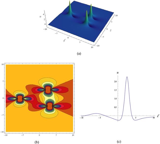
Similarly, we show in figure 9 the fourth-order rogue wave solution (97) with four interaction wave peaks. The highest two peaks are located at the center $(0,0),$ and the other entangled second highest wave peaks surround the center. Similar to the second- and third-order rogue waves in figures 3 and 5, the four interaction wave peaks in figure 9 gradually separate and give birth to another five wave peaks as long as one or all of $\theta $ and $\vartheta $ is/are given sufficiently large value(s). For example, see figures 10 and 11 for two symmetric fourth-order rogue waves, the one corresponding to $\theta =0$ and $\vartheta =6\times {10}^{7}$ is symmetric with respect to the line $z=0,$ and the other given $\theta =6\times {10}^{7}$ and $\vartheta =0$ is symmetric with respect to the line $\xi =0.$ However, the parameters $\theta =6\times {10}^{7}$ and $\vartheta =6\times {10}^{7}$ lead to an asymmetric fourth-order rogue wave, see figure 12.
Figure 9. Fourth-order rogue wave localized in (97) with $a=-4.6,$ $c=-3.15,$ $\alpha =3,$ $\beta =1,$ $\gamma =7,$ $\vartheta =0$ and $\theta =0,$ (a) 3D graph; (b) contour plot; (c) profile at $z=0.$
Figure 10. Fourth-order rogue wave localized in (97) with $a=-4.6,$ $c=-3.15,$ $\alpha =3,$ $\beta =1,$ $\gamma =7,$ $\theta =0$ and $\vartheta =6\times {10}^{7},$ (a) 3D graph; (b) contour plot; (c) profile at $z=0.$
Figure 11. Fourth-order rogue wave localized in (97) with $a=-4.6,$ $c=-3.15,$ $\alpha =3,$ $\beta =1,$ $\gamma =7,$ $\theta =6\times {10}^{7}$ and $\vartheta =0,$ (a) 3D graph; (b) contour plot; (c) profile at $z=0.$
Figure 12. Fourth-order rogue wave localized in (97) with $a=-4.6,$ $c=-3.15,$ $\alpha =3,$ $\beta =1,$ $\gamma =7,$ $\theta =6\times {10}^{7}$ and $\vartheta =6\times {10}^{7},$ (a) 3D graph; (b) contour plot; (c) profile at $\xi =10.$

5. Conclusion and discussion

In summary, we have constructed first-, second-, third- and fourth-order rogue wave solutions (30), (39), (55) and (97) of the (3 + 1)-dimensional gB equation (1) through Zhaqilao's symbolic calculation approach [22]. To the best of our knowledge, the high-order rogue wave solutions (39), (55) and (97) are new. This paper shows that the two parameters $\theta $ and $\vartheta $ included in solutions (30), (39), (55) and (97) control the following aspects:

(1) The center $(\theta ,\vartheta )$ of the first-order rogue wave solution (30).

(2) The fission giving birth to more wave peaks of the second-, third- and fourth-order rogue wave solutions (39), (55) and (97), the larger the value of $\theta $ and $\vartheta ,$ the larger the distance between the wave peaks

(3) The symmetry of high-order rogue wave solutions (39), (55) and (97), the rules of which are that when one or all of $\theta $ and $\vartheta $ are zero(s) then these rogue wave solutions are symmetric with respect to the line $z=0$ when $\theta =0$ or the line $\xi =0$ when $\vartheta =0,$ but asymmetric for $\theta \vartheta \ne 0.$

In view of the controllability of parameters $\theta $ and $\vartheta $ on the center, fission and asymmetry of first-, second-, third- and fourth-order rogue wave solutions (30), (39), (55) and (97), we can consider their potential applications in physics, such as the design of adjustable resistors and controllable switching devices under specific environment or with special requirements. Since the gB equation (1) or its reduced equation (23) is a kind of fluid equation, if the fluid is assumed to be a conductive liquid, we can not only use the vibration of the wave peak to trigger the connected power supply, but also adjust the size of the resistance by adjusting the number of fission wave peaks, so as to achieve the purpose of designing adjustable resistance and controllable switching device. If feasible, we can also consider using the controllability of wave crest position and asymmetry of rogue wave solutions (30), (39), (55) and (97) to design adjustable resistors and controllable switching devices that meet other conditions including the horizontal position and vertical height design of the device electric shock point. Nonetheless, we are still looking forward to other physical applications of these obtained rogue wave solutions with controllable center, fission and asymmetry.
For the method [22], it is a novel and meaningful discovery that the fission and asymmetry of higher-order rouge waves can be controlled by the embedded parameters $\theta $ and $\vartheta .$ High asymmetry is an important observation point in the study of rogue waves. Although the rogue wave solutions obtained in this paper have asymmetric controllability, there is still a certain distance from the highly asymmetric rogue waves, which raises a problem worthy of study for our next work. Nonlinear problems are always full of infinite charm and challenges. Some meaningful developments of nonlinear models deserve attention, such as the H2 optimal controller of coupled stochastic algebraic Riccati equations [32], and the influence of higher-order nonlinear effects on optical solitons [33].

We would like to thank the Editor and three anonymous referees for the helpful comments. This work was supported by Liaoning BaiQianWan Talents Program of China (LRS2020[78]), the Natural Science Foundation of Education Department of Liaoning Province of China (LJ2020002) and the National Natural Science Foundation of China (11547005).

1
Guo B L Tian L X Yan Z Y Ling L M 2015 Rogue Wave and Its Mathematical Theory Hangzhou Zhejiang Science and Technology Press

2
Draper L 1965 Freak wave Mar. Obs. 35 193

3
Solli D R Ropers C Koonath P Jalali B 2007 Optical rogue waves Nature 450 1054

DOI

4
Akhmediev N Ankiewicz A Soto-Crespo J M 2009 Rogue waves and rational solutions of the nonlinear Schrödinger equation Phys. Rev. E 80 026601

DOI

5
Yan Z Y 2010 Financial rogue waves Commun. Theor. Phys. 54 947

DOI

6
Guo B L Ling L M 2011 Rogue wave, breathers and bright-dark-rogue solutions for the coupled Schrödinger equations Chin. Phys. Lett. 28 110202

DOI

7
Guo B L Ling L M Liu Q P 2012 Nonlinear Schrödinger equation: Generalized Darboux transformation and rogue wave solutions Phys. Rev. E 85 026607

DOI

8
Ohta Y Yang J K 2012 General high-order rogue waves and their dynamics in the nonlinear Schrödinger equation P. Roy. Soc. A-Math. Phys. 468 1716

DOI

9
Wang X B Tian S F Qin C Y Zhang T T 2016 Characteristics of the breathers, rogue waves and solitary waves in a generalized (2+1)-dimensional Boussinesq equation Europhys. Lett. 115 10002

DOI

10
Randoux S Suret P El G 2016 Inverse scattering transform analysis of rogue waves using local periodization procedure Sci. Rep. 6 29238

DOI

11
Chen S Y Yan Z Y 2019 The higher-order nonlinear Schrödinger equation with non-zero boundary conditions: Robust inverse scattering transform, breathers, and rogons Phys. Lett. A 383 125906

DOI

12
Zhang S Zhang L J Xu B 2019 Rational waves and complex dynamics: Analytical insights into a generalized nonlinear Schrödinger equation with distributed coefficients Complexity 2019 3206503

DOI

13
Chen M Li B Yu Y X 2019 Darboux transformations, higher-order rational solitons and rogue wave solutions for a (2+1)-dimensional nonlinear Schrödinger equation Commun. Theor. Phys. 71 027

DOI

14
Dai C Q Wang Y Y Zhang J F 2020 Managements of scalar and vector rogue waves in a partially nonlocal nonlinear medium with linear and harmonic potentials Nonlinear Dyn 102 379

DOI

15
Peng W Q Pu J C Chen Y 2022 PINN deep learning method for the Chen–Lee–Liu equation: Rogue wave on the periodic background Commun. Nonlinear. Sci. Numer. Simul. 105 106067

DOI

16
Ma W X 2021 A polynomial conjecture connected with rogue waves in the KdV equation Part. Diff. Equ. Appl. Math. 3 100023

DOI

17
Zhang H Y Zhang Y F 2021 Breathers and multiple rogue waves solutions of the (3+1)-dimensional Jimbo-Miwa equation Mod. Phys. Lett. B 35 2150183

DOI

18
Lou Y Zhang Y Ye R S Li M 2021 Solitons and dynamics for the integrable nonlocal pair-transition-coupled nonlinear Schrödinger equation Appl. Math. Comput. 409 126417

DOI

19
Li B Q Ma Y L 2021 Extended generalized Darboux transformation to hybrid rogue wave and breather solutions for a nonlinear Schrödinger equation Appl. Math. Comput. 386 125469

DOI

20
Zhang R F Li M C Albishari M Zheng F C Lan Z Z 2021 Generalized lump solutions, classical lump solutions and rogue waves of the (2+1)-dimensional Caudrey-Dodd-Gibbon-Kotera-Sawada-like equation Appl. Math. Comput. 403 126201

DOI

21
Zhaqilao 2013 Rogue waves and rational solutions of a (3+1)-dimensional nonlinear evolution equation Phys. Lett. A 377 3021

DOI

22
Zhaqilao 2018 A symbolic computation approach to constructing rogue waves with a controllable center in the nonlinear systems Comput. Math. Appl. 75 3331

DOI

23
Cao Y L Tian H Ghanbari B 2021 On constructing of multiple rogue wave solutions to the (3+1)-dimensional Korteweg-de Vries Benjamin-Bona-Mahony equation Phys. Scripta 96 035226

DOI

24
Wang M Tian B Sun Y Zhang Z 2020 Lump, mixed lump-stripe and rogue wave-stripe solutions of a (3+1)-dimensional nonlinear wave equation for a liquid with gas bubbles Comput. Math. Appl. 79 576

DOI

25
Sun B N Wazwaz A M 2018 General high-order breathers and rogue waves in the (3+1)-dimensional KP-Boussinesq equation Commun. Nonlinear. Sci. Numer. Simul. 64 1

DOI

26
Liu W H Zhang Y F 2019 Multiple rogue wave solutions of the (3+1)-dimensional Kadomtsev-Petviashvili-Boussinesq equation Z. Angew. Math. Phys. 70 112

DOI

27
Yan X W 2019 Generalized (3+1)-dimensional Boussinesq equation: Breathers, rogue waves and their dynamics Mod. Phys. Lett. B 34 2050003

DOI

28
Hu Z Tang W Y Xue H X Zhang X Y Wang K P 2017 Numerical study of rogue wave overtopping with a fully-coupled fluid-structure interaction model Ocean Eng 137 48

DOI

29
Du Z Tian B Qu Q X Zhao X H 2020 Lax pair and vector semi-rational nonautonomous rogue waves for a coupled time-dependent coefficient fourth-order nonlinear Schrödinger system in an inhomogeneous optical fiber Chin. Phys. B 29 030202

DOI

30
Li Z D Huo C Z Li Q Y He P B Xu T F 2018 Symmetry and asymmetry rogue waves in two-component coupled nonlinear Schrödinger equations Chin. Phys. B 27 040505

DOI

31
Hirota R 2004 The Direct Method in Soliton Theory Cambridge Cambridge University Press

32
Ma H J Wang Y 2022 Full information H2 control of borel-measurable markov jump systems with multiplicative noises Mathematics 10 37

DOI

33
Wang R R Wang Y Y Dai C Q 2022 Influence of higher-order nonlinear effects on optical solitons of the complex Swift-Hohenberg model in the mode-locked fiber laser Opt. Laser. Technol. 152 108103

DOI

Outlines

/