


1. Introduction
In order to obtain the information of an unknown quantum state, we need to perform a complete measurement of the target quantum state, that is, quantum state tomography (QST). In the standard QST, a set of complete measurement bases and a state reconstruction algorithm are essential. However, with the expansion of the dimensions of quantum systems, the number of measurement bases required by QST increases exponentially. This will increase the complexity of the actual experiment because QST is a global reconstruction of all the information of the quantum state. Due to the existence of statistical errors, optimization methods are usually used to reconstruct the target quantum state, which is closest to the probability distribution of the measurement results [1, 2].
But in some cases, such as the verification of quantum entanglement [3] and quantum coherence [4], we only need partial information of the quantum state, so the traditional QST will be complex. Direct measurement schemes allow us to only obtain the information we are interested in because it does not require a global quantum state reconstruction. This will reduce the complexity of the practical experiment. Direct tomography schemes based on weak measurements have been developed recently [5–10]. In addition to important applications in the field of precision measurement [11–15], weak measurements also play an important role in direct measurement schemes. Lundeen et al [16] used weak measurements to directly measure the spatial wave function of photons. Malik et al [17] used the scheme to realize the direct measurement of 27-dimensional wave functions of photon orbital angular momentum. Wu et al [18] proposed a scheme for direct measurement of partial elements in general quantum states. Ren et al [19] proposed a weak measurement scheme for directly measuring arbitrary elements of a state density matrix, and extended it to the direct measurement of the multi-particle density matrix. Subsequently, in order to make up for decreased measurement precision caused by weak-coupling approximation in weak measurement, strong measurement schemes have also been proposed one after another [20–22]. But even so, direct measurement schemes based on weak or strong measurements require the coupling between target quantum states and extra auxiliary states, so it will increase the complexity of practical experiments. In addition, since there is a post-selection process in the measurement, it will consume a lot of measurement resources and reduce the utilization.
In order to avoid the disadvantages of weak-value-based schemes, this paper proposes a direct measurement scheme without auxiliary states for a single-particle system. Subsequently, we extend this scheme to the direct measurement of a multi-particle system. Since our scheme does not require auxiliary states and post-selection process, it will reduce the complexity of practical experiments. Meanwhile, our scheme is easy to be expanded and integrated, which is helpful for the realization of direct quantum tomography in integrated quantum chips. The paper is organized as follows: in section 2 , we propose a direct quantum tomography scheme without auxiliary states for arbitrary systems and complete the error analysis in section 3 . Finally, in section 4 , when we take into account the dephasing of quantum states caused by noise channels, we modify the circuits and the modified circuits are still applicable to the dephasing situation.
2. Quantum circuits for directly measuring the general quantum states
In this section, we first introduce a direct measurement scheme without auxiliary states for single-qubit systems. We then generalize it to arbitrary multi-qubit systems. To demonstrate the advantages of circuit schemes, we compare this scheme with a direct measurement scheme based on weak measurements. In the weak measurement scheme, in order to realize the direct measurement of a single-qubit unknown state, two auxiliary states and two couplings need to be used as shown in figure 1(a). For direct measurement of multiple qubits, we will need more auxiliary states and couplings, which will increase the complexity of practical experiments. In addition, in some physical systems, these required auxiliary states are not easy to be constructed [19], and the required couplings are not easy to achieve, which will limit the application of weak measurement schemes. In our circuit scheme shown in figure 1(b), auxiliary states are not necessary and the required basic quantum gates are already implemented well by many physical systems, so this will reduce the complexity of practical applications. Next, we will show in detail how our scheme works.
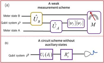
Figure 1. Two schemes for directly measuring single-qubit systems. (a) A weak measurement scheme for directly measuring specific matrix elements. In this scheme, additional auxiliary states need to be used, and more auxiliary states are needed when the target quantum state is a multi-particle system. (b) A circuit scheme without auxiliary state. Here ${U}_{l}\left(\delta \right)$ represents a single-qubit phase-shift gate, and ${R}_{y}^{+}$ represents a rotation gate, satisfying ${R}_{y}^{+}=\exp \left({\rm{i}}\pi {\hat{\sigma }}_{y}/4\right).$ ${R}_{y}^{+}$ is an inverse operator of the operator ${R}_{y}.$ |
As for a single-qubit state, we could describe this quantum system with a density operator, i.e. $\hat{\rho }=\displaystyle {\sum }_{m,n}{\lambda }_{mn}{{\rm{e}}}^{{\rm{i}}{\theta }_{mn}}\left|m\right\rangle \left\langle n\right|,$ where $m,n\in \left\{0,1\right\}.$ Since the density operator is a Hermitian operator, so ${\theta }_{nn}=0,{\theta }_{mn}=-{\theta }_{nm},{\lambda }_{mn}={\lambda }_{nm}.$ To obtain the diagonal elements of the density operator, we can directly use the projective operator $\left|n\right\rangle \left\langle n\right|.$ However, it is a challenge to measure non-diagonal elements because the operator $\left|m\right\rangle \left\langle n\right|\left(m\ne n\right)$ is not a Hermitian operator. At this point, we can use the scheme shown in figure 1(b) to obtain non-diagonal elements. In this scheme, we need to perform a phase shift operation on the target quantum state, and its operator can be expressed as
$\begin{eqnarray}{U}_{l}\left({\delta }_{l}\right)=1+\left({{\rm{e}}}^{{\rm{i}}{\delta }_{l}}-1\right)\left|l\right\rangle \left\langle l\right|,\,l\in \left\{0,1\right\}.\end{eqnarray}$
After that, the output state ${\rho }_{{\rm{out}}}$ can be expressed as $\begin{eqnarray}\begin{array}{l}{\rho }_{{\rm{out}}}={U}_{l}\rho {U}_{l}^{+}={\lambda }_{ln}{{\rm{e}}}^{{\rm{i}}\left({\theta }_{ln}+{\delta }_{l}\right)}\left|l\right\rangle \left\langle n\right|+{\lambda }_{ml}{{\rm{e}}}^{{\rm{i}}\left({\theta }_{ml}-{\delta }_{l}\right)}\left|m\right\rangle \left\langle l\right|\\ \,+{\lambda }_{mm}{{\rm{e}}}^{{\rm{i}}{\theta }_{mm}}\left|m\right\rangle \left\langle m\right|+{\lambda }_{ll}{{\rm{e}}}^{{\rm{i}}{\theta }_{ll}}\left|l\right\rangle \left\langle l\right|\left(m\ne l,n\ne l\right).\end{array}\end{eqnarray}$
We then choose the measurement basis $\hat{\mu }=\left|{\rm{\Phi }}\right\rangle \left\langle {\rm{\Phi }}\right|\,={R}_{y}\left|0\right\rangle \left\langle 0\right|{R}_{y}^{+}$ to measure the output state, where $\left|{\rm{\Phi }}\right\rangle \,=1/\sqrt{2}\left(\left|l\right\rangle +\left|n\right\rangle \right)\left(n\ne l\right).$ This projection measurement can be achieved by a single-qubit rotation gate ${R}_{y},$ satisfying ${R}_{y}\left|0\right\rangle ={{\rm{e}}}^{-{\rm{i}}\pi {\hat{\sigma }}_{y}/4}\left|0\right\rangle =\left|{\rm{\Phi }}\right\rangle ,$ and a Pauli measurement $\left|0\right\rangle \left\langle 0\right|.$ Here, ${\hat{\sigma }}_{y}$ is a Pauli operator. Thus, we can get the value of projective probability $P$ as follows $\begin{eqnarray}P={\rm{Tr}}\left(\hat{\mu }{\hat{\rho }}_{{\rm{out}}}\right)=\displaystyle \frac{{\lambda }_{nn}+{\lambda }_{ll}}{2}+{\lambda }_{ln}\,\cos \left({\delta }_{l}+{\theta }_{ln}\right).\end{eqnarray}$
When choosing the imposed phase shift ${\delta }_{l}$ as $0,\pi /2,\pi ,3\pi /2,$ we denote the corresponding projected probability as ${P}_{0},{P}_{\pi /2},{P}_{\pi },{P}_{3\pi /2},$ respectively. Then we can obtain the real and imaginary parts of any off-diagonal elements by the following equations $\begin{eqnarray}\mathrm{Re}\left({\rho }_{ln}\right)={\lambda }_{ln}\,\cos \,{\theta }_{ln}=\left({P}_{0}-{P}_{\pi }\right)/2,\end{eqnarray}$
$\begin{eqnarray}{\rm{Im}}\left({\rho }_{ln}\right)={\lambda }_{ln}\,\sin \,{\theta }_{ln}=\left({P}_{3\pi /2}-{P}_{\pi /2}\right)/2.\end{eqnarray}$
Next, we generalize this scheme to the measurement of arbitrary multi-qubit systems. Multi-qubit states can exhibit quantum entanglement and quantum nonlocality, so measuring a multi-qubit system will become complicated. As we all know, a multi-qubit system can be expressed as ${\hat{\rho }}_{N}\,=\displaystyle {\sum }_{{s}_{1}\cdots {s}_{N},{s^{\prime} }_{1}\cdots {s^{\prime} }_{N}}{\lambda }_{{s}_{1}\cdots {s}_{N}}^{{s^{\prime} }_{1}\cdots {s^{\prime} }_{N}}{{\rm{e}}}^{{\rm{i}}{\theta }_{{s}_{1}\cdots {s}_{N}}^{{s^{\prime} }_{1}\cdots {s^{\prime} }_{N}}}\left|{s}_{1},\cdots {s}_{N}\right\rangle \left\langle {s^{\prime} }_{1},\cdots {s^{\prime} }_{N}\right|,$ where ${s}_{1},{s}_{2}\cdots {s}_{N},{s^{\prime} }_{1},{s^{\prime} }_{2}\cdots {s^{\prime} }_{N} $ $ \in \left\{0,1\right\}.$ At this time, the single-qubit phase-shift gate we need is extended to a multi-qubit phase-shift gate (see figure 2). The expression for this multi-qubit phase-shift gate is $\begin{eqnarray}\begin{array}{l}{U}_{l}=1+\left[\exp \left({\rm{i}}{\delta }_{{s}_{1}^{{l}_{1}},\cdots {s}_{N}^{{l}_{N}}}\right)-1\right]\left|{s}_{1}^{{l}_{1}},\cdots {s}_{N}^{{l}_{N}}\right\rangle \left\langle {s}_{1}^{{l}_{1}},\cdots {s}_{N}^{{l}_{N}}\right|,\\ \,{s}_{1}^{{l}_{1}},\cdots {s}_{N}^{{l}_{N}}\in \left\{0,1\right\}.\end{array}\end{eqnarray}$
Then, the measurement basis we need at this time is ${\hat{\mu }}_{N}\,=\left|{{\rm{\Phi }}}_{N}\right\rangle \left\langle {{\rm{\Phi }}}_{N}\right|,$ where $\left|{{\rm{\Phi }}}_{N}\right\rangle =1/\sqrt{2}\left(\left|{s}_{1}^{{l}_{1}},\cdots {s}_{N}^{{l}_{N}}\right\rangle +\left|{s}_{1},\cdots {s}_{N}\right\rangle \right),$ $\left(\left|{s}_{1}^{{l}_{1}},\cdots {s}_{N}^{{l}_{N}}\right\rangle \ne \left|{s}_{1},\cdots {s}_{N}\right\rangle \right).$ The operator ${\hat{\mu }}_{N}$ can always be converted to a Pauli measurement by some single-qubit gates and two-qubit controlled-NOT gates, namely ${\hat{\mu }}_{N}\,=T\left|0\cdots 0\right\rangle \left\langle 0\cdots 0\right|{T}^{+}.$ We can see the projection measurement process is equivalent to the prepared process of the quantum state $\left|{{\rm{\Phi }}}_{N}\right\rangle $ by using the eigenstate $\left|0\cdots 0\right\rangle .$ The circuit structure of the operator ${T}^{+}$ depends on the quantum state $\left|{{\rm{\Phi }}}_{N}\right\rangle ,$ and the mathematical expression of the state $\left|{{\rm{\Phi }}}_{N}\right\rangle $ includes the entangled state form and the direct product state form. For instance, when the mathematical expression of the state $\left|{{\rm{\Phi }}}_{N}\right\rangle $ satisfies $\left|{{\rm{\Phi }}}_{N}\right\rangle =1/\sqrt{2}\left|{s}_{1}^{{l}_{1}}\right\rangle \otimes \cdots \left|{s}_{N}^{{l}_{N}}\right\rangle \left(\left|{s}_{i}^{{l}_{i}}\right\rangle +\left|{s}_{i}\right\rangle \right),$ where $i\in \left\{1,2,\cdots N\right\}$ and $\left({s}_{1}^{{l}_{1}}={s}_{1},\cdots {s}_{N}^{{l}_{N}}={s}_{N},{s}_{i}^{{l}_{i}}\ne {s}_{i}\right),$ at this time $\left|{{\rm{\Phi }}}_{N}\right\rangle $ is a separable state which can be prepared by the quantum circuit in figure 2(b). When the quantum state $\left|{{\rm{\Phi }}}_{N}\right\rangle $ satisfies $\left|{{\rm{\Phi }}}_{N}\right\rangle =1/\sqrt{2}\left|{s}_{1}^{{l}_{1}}\right\rangle \otimes \cdots \left|{s}_{i-1}^{{l}_{i-1}}\right\rangle \otimes \left(\left|{s}_{1}^{{l}_{1}},\cdots {s}_{N}^{{l}_{N}}\right\rangle \right.+\left.\left|{s}_{1},\cdots {s}_{N}\right\rangle \right),$ where $({s}_{1}^{{l}_{1}}={s}_{1},\cdots {s}_{i-1}^{{l}_{i-1}}={s}_{i-1},$ $\text{}{s}_{i}^{{l}_{i}}\ne {s}_{i}),$ it is a partially entangled state and it can be prepared by the quantum circuit shown in figure 2(c). Similarly, when $\left|{{\rm{\Phi }}}_{N}\right\rangle \,=1/\sqrt{2}\left(\left|{s}_{1}^{{l}_{1}},\cdots {s}_{N}^{{l}_{N}}\right\rangle +\left|{s}_{1},\cdots {s}_{N}\right\rangle \right)\left({s}_{1}^{{l}_{1}}\ne {s}_{1},\cdots {s}_{N}^{{l}_{N}}\ne {s}_{N}\right),$ it is a fully entangled state which can be prepared by the quantum circuit shown in figure 2(d).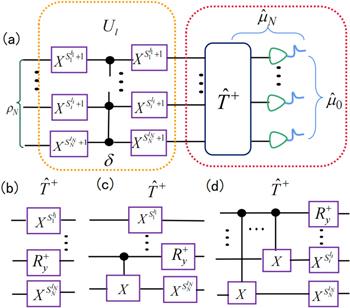
Figure 2. A circuit scheme to realize the direct measurement of arbitrary multi-qubit systems. (a) A complete operation flow; (b) The circuit structure of the operator ${T}^{+}$ when the state $\left|{{\rm{\Phi }}}_{N}\right\rangle $ is a direct product state (c) The circuit structure of the operator ${T}^{+}$ when the state $\left|{{\rm{\Phi }}}_{N}\right\rangle $ is partially entangled. (d) The circuit structure of the operator ${T}^{+}$ when the state $\left|{{\rm{\Phi }}}_{N}\right\rangle $ is fully entangled. Here X represents a single-qubit NOT gate. |
After completing the projection measurement ${\hat{\mu }}_{N},$ we can get the projection probability as4 ), (5 ).
$\begin{eqnarray}\begin{array}{l}P={\rm{Tr}}\left[{T}^{+}{U}_{l}{\hat{\rho }}_{N}{U}_{l}^{+}T\left|0\cdots 0\right\rangle \left\langle 0\cdots 0\right|\right]\\ =\,\displaystyle \frac{{\lambda }_{{s}_{1}\cdots {s}_{N}}^{{s}_{1}\cdots {s}_{N}}+{\lambda }_{{s}_{1}^{{l}_{1}},\cdots {s}_{N}^{{l}_{N}}}^{{s}_{1}^{{l}_{1}},\cdots {s}_{N}^{{l}_{N}}}}{2}+{\lambda }_{{s}_{1}^{{l}_{1}},\cdots {s}_{N}^{{l}_{N}}}^{{s}_{1}\cdots {s}_{N}}\,\cos \left[{\delta }_{{s}_{1}^{{l}_{1}},\cdots {s}_{N}^{{l}_{N}}}+{\theta }_{{s}_{1}^{{l}_{1}},\cdots {s}_{N}^{{l}_{N}}}^{{s}_{1}\cdots {s}_{N}}\right].\end{array}\end{eqnarray}$
Similarly, when we choose the imposed phase shifts ${\delta }_{l}$ as $0,\,\pi /2,\,\pi ,\,3\pi /2,$ we denote the corresponding projection probability as ${P}_{0},\,{P}_{\pi /2},{P}_{\pi },{P}_{3\pi /2},$ respectively. We then can obtain the real and imaginary parts of arbitrary off-diagonal matrix elements like equations ( $\begin{eqnarray}\begin{array}{l}\mathrm{Re}\left(\left\langle {s}_{1}^{{l}_{1}},\cdots {s}_{N}^{{l}_{N}}\right|\rho \left|{s}_{1},\cdots {s}_{N}\right\rangle \right)\\ ={\lambda }_{{s}_{1}^{{l}_{1}},\cdots {s}_{N}^{{l}_{N}}}^{{s}_{1}\cdots {s}_{N}}\,\cos \,{\theta }_{{s}_{1}^{{l}_{1}},\cdots {s}_{N}^{{l}_{N}}}^{{s}_{1}\cdots {s}_{N}}=\displaystyle \frac{{P}_{0}-{P}_{\pi }}{2},\end{array}\end{eqnarray}$
$\begin{eqnarray}\begin{array}{l}\text{Im}\left(\left\langle {s}_{1}^{{l}_{1}},\cdots {s}_{N}^{{l}_{N}}\right|\rho \left|{s}_{1},\cdots {s}_{N}\right\rangle \right)\\ ={\lambda }_{{s}_{1}^{{l}_{1}},\cdots {s}_{N}^{{l}_{N}}}^{{s}_{1}\cdots {s}_{N}}\,\sin \,{\theta }_{{s}_{1}^{{l}_{1}},\cdots {s}_{N}^{{l}_{N}}}^{{s}_{1}\cdots {s}_{N}}=\displaystyle \frac{{P}_{3\pi /2}-{P}_{\pi /2}}{2}.\end{array}\end{eqnarray}$
In order to show our circuit scheme more clearly, here we take a three-qubit system as an example to show the circuit scheme how to work. When the matrix elements we need to measure are $\left\langle 100\right|\rho \left|110\right\rangle ,$ $\left\langle 010\right|\rho \left|101\right\rangle ,$ $\left\langle 000\right|\rho \left|011\right\rangle ,$ and $\left\langle 000\right|\rho \left|010\right\rangle ,$ we only need to perform these circuits shown in figures 3(a)–(c) respectively.
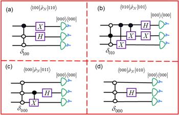
Figure 3. Circuit schemes of measuring specific matrix elements for a three-qubit system. (a) is the quantum circuit that directly measures the matrix element $\left\langle 100\right|\rho \left|110\right\rangle .$ (b) is the quantum circuit that directly measures the matrix element $\left\langle 010\right|\rho \left|101\right\rangle .$ (c) is the quantum circuit that directly measures the matrix element $\left\langle 000\right|\rho \left|011\right\rangle .$ (d) is the quantum circuit that directly measures the matrix element $\left\langle 000\right|\rho \left|010\right\rangle .$ |
It is worth mentioning that this scheme is also applicable to high-dimensional quantum state systems, namely qudit systems, such as photon orbital angular momentum. We only need some corresponding high-dimensional quantum gates to implement the circuit structure in figure 2 to obtain any specific matrix elements of the high-dimensional quantum system. Since the measurement steps are similar to those in figure 2, here we directly give the direct measurement circuit of the high-dimensional qudit systems (see figure 4).
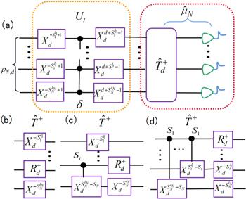
Figure 4. (a) A circuit diagram for direct measurement of a d-dimensional $\left(d\gt 2\right)$ quantum system. The measurement flow is similar to the steps in figure 2. In this scheme, some high-dimensional single-qudit gates and two-qudit controlled-NOT gates are used. ${X}_{d}^{{S}_{i}}$ and ${R}_{d}^{+}$ are respectively a single-qudit NOT gate and a single-qudit rotation gate, satisfying ${X}_{d}^{d}=1,$ ${X}_{d}^{{S}_{i}}\left|i\right\rangle =\left|i\oplus {S}_{i}\right\rangle $ and ${R}_{d}^{+}{\left(\left(\left|{s}_{i}^{{l}_{i}}\right\rangle +\left|{s}_{i}\right\rangle \right)/\sqrt{2}\right)}_{d}={\left|0\right\rangle }_{d}.$ Here, the subscript d represents a d-dimensional quantum system. (b) The circuit structure of the operator ${T}_{d}^{+}$ when the state ${\left|{{\rm{\Phi }}}_{N}\right\rangle }_{d}$ is a direct product state. (c) The circuit structure of the operator ${T}_{d}^{+}$ when the state ${\left|{{\rm{\Phi }}}_{N}\right\rangle }_{d}$ is partially entangled. (d) The circuit structure of the operator ${T}_{d}^{+}$ when the state ${\left|{{\rm{\Phi }}}_{N}\right\rangle }_{d}$ is fully entangled. |
3. Error analysis of direct measurement scheme
In this section, we present the measurement error analysis of the circuit scheme. Here we take the pure state as an example to analyze the measurement error. As we know, a pure state can be expressed as $\left|{\psi }_{N}\right\rangle =\displaystyle {\sum }_{s}{a}_{s}{{\rm{e}}}^{{\rm{i}}{\theta }_{s}}\left|{s}_{1},\cdots {s}_{N}\right\rangle $ = $\displaystyle {\sum }_{i}{A}_{i}\left|{s}_{1},\cdots {s}_{N}\right\rangle ,$ where ${s}_{1},\cdot \cdot \cdot {s}_{N}\in \left\{0,1\right\},$ Ai is a complex number, satisfying ${A}_{i}={a}_{s}{{\rm{e}}}^{{\rm{i}}{\theta }_{s}}.$ ${a}_{s}$ and ${\theta }_{s}$ are the amplitude and the phase of the expansion coefficients, respectively. For the convenience of writing, we let ${A}_{i}^{R}=\mathrm{Re}\left({A}_{i}\right),{A}_{i}^{I}={\rm{Im}}\left({A}_{i}\right),$ so we can get the real part and the imaginary part of any expansion coefficients by the following equations
$\begin{eqnarray}{A}_{i}^{R}=\left({P}_{0}-{P}_{\pi }\right)/\left(2{a}_{0}\right),\end{eqnarray}$
$\begin{eqnarray}{A}_{i}^{I}=\left({P}_{3\pi /2}-{P}_{\pi /2}\right)/\left(2{a}_{0}\right).\end{eqnarray}$
As for the value of ${a}_{0},$ we can directly obtain it by a Pauli measurement $\left|0\cdots 0\right\rangle \left\langle 0\cdots 0\right|.$ According to the error transfer formula, we can get the measurement error ${\rm{\Delta }}{A}_{i}^{R}$ and ${\rm{\Delta }}{A}_{i}^{I}$ as follows $\begin{eqnarray}\begin{array}{l}{\rm{\Delta }}{A}_{i}^{R}\\ =\sqrt{\displaystyle \frac{1}{4}+\displaystyle \frac{{a}_{s}^{2}}{4{a}_{0}^{2}}-\displaystyle \frac{{\left({a}_{0}^{2}+{a}_{s}^{2}\right)}^{2}}{8{a}_{0}^{2}}-\displaystyle \frac{{a}_{s}^{2}{\cos }^{2}{\theta }_{s}}{2}+\displaystyle \frac{{a}_{s}^{2}{\cos }^{2}{\theta }_{s}\left(1-{a}_{0}^{2}\right)}{4{a}_{0}^{2}}},\end{array}\end{eqnarray}$
$\begin{eqnarray}\begin{array}{l}{\rm{\Delta }}{A}_{i}^{I}\\ =\sqrt{\displaystyle \frac{1}{4}+\displaystyle \frac{{a}_{s}^{2}}{4{a}_{0}^{2}}-\displaystyle \frac{{\left({a}_{0}^{2}+{a}_{s}^{2}\right)}^{2}}{8{a}_{0}^{2}}-\displaystyle \frac{{a}_{s}^{2}{\sin }^{2}{\theta }_{s}}{2}+\displaystyle \frac{{a}_{s}^{2}{\sin }^{2}{\theta }_{s}\left(1-{a}_{0}^{2}\right)}{4{a}_{0}^{2}}}.\end{array}\end{eqnarray}$
According to Fisher information theory, we can get the Cramér–Rao bound of the measurement error as ${\rm{\Delta }}{A}_{Q\mathrm{CRB}}^{R}={\rm{\Delta }}{A}_{Q\mathrm{CRB}}^{I}=1/\left(2\sqrt{1-{a}_{s}^{2}}\right).$ The Cramér–Rao bound defines the minimum measurement error that can be achieved in our parameter measurement process, and it determines the lower bound of measurement error. If the measurement error of our scheme is close to the Cramér–Rao bound, it indicates that our scheme has a high measurement precision.Figure 5(a) shows the relationship among the ratio ${\rm{\Delta }}{A}_{\mathrm{QCRB}}^{R}/{\rm{\Delta }}{A}_{i}^{R},$ ${a}_{s}$ and ${\theta }_{s}.$ When we fix the value of ${a}_{s},$ we can see periodic changes of the ratio ${\rm{\Delta }}{A}_{Q\mathrm{CRB}}^{R}/{\rm{\Delta }}{A}_{i}^{R},$ which can be verified by equation (13 ). It can also be seen that when the values of ${a}_{s}$ and ${\theta }_{s}$ are within a certain range, the measurement precision of our circuit scheme can be very close to the Cramér–Rao bound, and similar results are shown in figure 5(b).
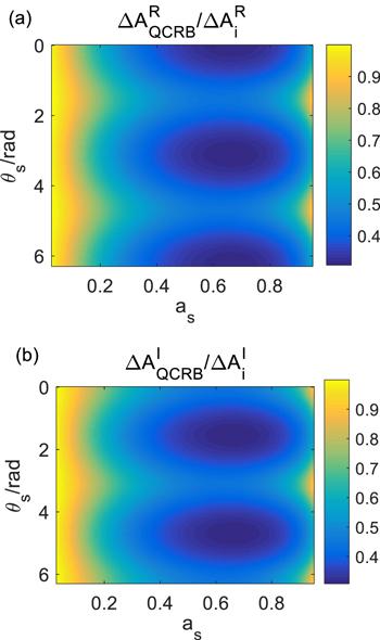
Figure 5. (a) The ratio ${\rm{\Delta }}{A}_{Q\mathrm{CRB}}^{R}/{\rm{\Delta }}{A}_{i}^{R}$ as a function of ${a}_{s}$ and ${\theta }_{s}.$ (b) The ratio ${\rm{\Delta }}{A}_{Q\mathrm{CRB}}^{I}/{\rm{\Delta }}{A}_{i}^{I}$ as a function of ${a}_{s}$ and ${\theta }_{s}.$ Here ${a}_{0}$ is chosen to be 0.2. |
4. Quantum circuits of direct measurement against dephasing
Two-level systems are often commonly used in quantum information. The entangled pure states of multi-qubit are important resources in the field of quantum information. However, an entangled pure state, the expression of which satisfies $\left|{\psi }_{N}\right\rangle =\displaystyle {\sum }_{s}{a}_{s}{{\rm{e}}}^{{\rm{i}}{\theta }_{s}}\left|{s}_{1},\cdots {s}_{N}\right\rangle ,$ is easy to be affected by noise. In this section, we will analyze the impact of environmental noise on the target quantum state and propose corresponding solutions. In the measurement process of multi-qubit pure states, due to the existence of noisy channels between part A and part B (see figure 6(a)), dephasing will occur in the target quantum state. At this time, the non-diagonal elements of the density matrix of the target quantum state will gradually degenerate, so that we cannot get the phase values of expansion coefficients of the multi-qubit pure states. After dephasing, the output quantum state at this time becomes ${\hat{\rho }}_{i}=\displaystyle {\sum }_{{s}_{1,\cdots }{s}_{N}}{a}_{{s}_{1},\cdots {s}_{N}}^{2}\left|{s}_{1},\cdots {s}_{N}\right\rangle \left\langle {s}_{1},\cdots {s}_{N}\right|.$ There are only diagonal elements in the density matrix and we will not observe the phase values of expansion coefficients even if we perform a projection measurement. At the same time, the quantum Fisher information of the phase measurement is also 0. In order to obtain the phase information of the target quantum state under the condition of dephasing, we modify the circuits in section 2 (see figure 6(b)).
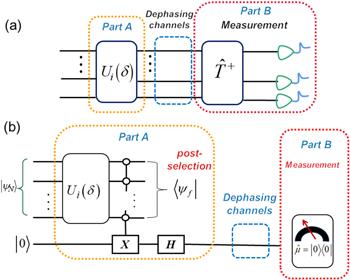
Figure 6. (a) Quantum circuits with dephasing channels. (b) Quantum circuits for measuring multi-qubit pure states when dephasing is considered. The original auxiliary state is $\left|0\right\rangle .$ Here, H represents a Hadamard gate. |
In the modified circuits, we use an auxiliary qubit to complete the direct measurement scheme in the dephasing situation. At this time, the joint quantum state of the auxiliary qubit and the target quantum state after the operation ${U}_{i}\left(\delta \right)$ is expressed as17 ). Here, the successful probability of post-selection satisfies ${p}_{k}={\rm{Tr}}\left(\left|{\psi }_{f}\right\rangle \left\langle {\psi }_{f}\right|{\rho }_{j}\right)\,=\left({a}_{0}^{2}+{a}_{s}^{2}\right)/2,$ where the density matrix of the joint state satisfies ${\rho }_{j}=\left|{\psi }_{j}\right\rangle \left\langle {\psi }_{j}\right|.$ For the convenience of writing, we let ${\theta }_{{s}_{1}^{{i}_{1}},\cdots {s}_{N}^{{i}_{N}}}={\theta }_{s},$ ${a}_{{s}_{1}^{{i}_{1}},\cdots {s}_{N}^{{i}_{N}}}={a}_{s},$ ${a}_{0\cdots 0}={a}_{0},$ ${\delta }_{{s}_{1}^{{i}_{1}},\cdots {s}_{N}^{{i}_{N}}}={\delta }_{s}.$ 23 ), ${\partial }_{{\theta }_{s}}{\lambda }_{i}=\partial {\lambda }_{i}/\partial {\theta }_{s},\left|{\partial }_{{\theta }_{s}}{\lambda }_{i}\right\rangle =\partial \left|{\lambda }_{i}\right\rangle /\partial {\theta }_{s}.$ The corresponding quantum Fisher information of the eigenstate $\left|{\lambda }_{i}\right\rangle $ satisfies ${F}_{Q,i}=4\left(\left\langle {\partial }_{{\theta }_{s}}{\lambda }_{i}| {\partial }_{{\theta }_{s}}{\lambda }_{i}\right\rangle -{\left|\,\left\langle {\partial }_{{\theta }_{s}}{\lambda }_{i}| {\lambda }_{i}\right\rangle \,\right|}^{2}\right).$ It can be seen from equation (21 ) that when the dephasing occurs completely, the quantum Fisher information of the density matrix $\rho ^{\prime} $ about the target phase ${\theta }_{s}$ is
$\begin{eqnarray}\begin{array}{l}\left|{\psi }_{i}\right\rangle =\left[{a}_{{s}_{1}^{{i}_{1}},\cdots {s}_{N}^{{i}_{N}}}\exp \left({\rm{i}}{\delta }_{{s}_{1}^{{i}_{1}},\cdots {s}_{N}^{{i}_{N}}}+{\rm{i}}{\theta }_{{s}_{1}^{{i}_{1}},\cdots {s}_{N}^{{i}_{N}}}\right)\left|{s}_{1}^{{i}_{1}},\cdots {s}_{N}^{{i}_{N}}\right\rangle \right.\\ \,+\left.\displaystyle {\sum }_{{s}_{1}\cdots {s}_{N}\ne {s}_{1}^{{i}_{1}}\cdots {s}_{N}^{{i}_{N}}}{a}_{{s}_{1},\cdots {s}_{N}}{{\rm{e}}}^{{\rm{i}}{\theta }_{{s}_{1},\cdots {s}_{N}}}\left|{s}_{1},\cdots {s}_{N}\right\rangle \right]\otimes \left|0\right\rangle .\end{array}\end{eqnarray}$
Next, a multi-qubit controlled-NOT gate is used to realize the coupling between the target state and the auxiliary state, and at this time the joint quantum state becomes $\begin{eqnarray}\begin{array}{l}\left|{\psi }_{j}\right\rangle ={a}_{{s}_{1}^{{i}_{1}},\cdots {s}_{N}^{{i}_{N}}}\exp \left({\rm{i}}{\delta }_{{s}_{1}^{{i}_{1}},\cdots {s}_{N}^{{i}_{N}}}+{\rm{i}}{\theta }_{{s}_{1}^{{i}_{1}},\cdots {s}_{N}^{{i}_{N}}}\right)\left|{s}_{1}^{{i}_{1}},\cdots {s}_{N}^{{i}_{N}}\right\rangle \otimes \left|0\right\rangle \\ +\,\displaystyle {\sum }_{{s}_{1}\cdots {s}_{N}\ne {s}_{1}^{{i}_{1}}\cdots {s}_{N}^{{i}_{N}}}{a}_{{s}_{1},\cdots {s}_{N}}{{\rm{e}}}^{{\rm{i}}{\theta }_{{s}_{1},\cdots {s}_{N}}}\left|{s}_{1},\cdots {s}_{N}\right\rangle \otimes \left|0\right\rangle \\ +\,{a}_{0\cdots 0}\left|0\cdots 0\right\rangle \otimes \left|1\right\rangle .\end{array}\end{eqnarray}$
Subsequently, we perform a post-selection process on the target quantum state, the purpose of which is to pick up the target eigenstate $\left|{s}_{1}^{{i}_{1}},\cdots {s}_{N}^{{i}_{N}}\right\rangle $ and eigenstate $\left|00\cdots 0\right\rangle ,$ so the expression of the post-selection state we need is as follows $\begin{eqnarray}\left|{\psi }_{f}\right\rangle =1/\sqrt{2}\left(\left|0\cdots 0\right\rangle +\left|{s}_{1}^{{i}_{1}},\cdots {s}_{N}^{{i}_{N}}\right\rangle \right)\left({s}_{1}^{{i}_{1}},\cdots {s}_{N}^{{i}_{N}}\ne 0\right).\end{eqnarray}$
After the post-selection, the quantum state $\left|\varphi \right\rangle $ of the auxiliary qubit is described by equation ( $\begin{eqnarray}\left|\varphi \right\rangle =\displaystyle \frac{\left\langle {\psi }_{f}| {\psi }_{j}\right\rangle }{\sqrt{{p}_{k}}}=\displaystyle \frac{1}{\sqrt{2{p}_{k}}}\left({a}_{0}\left|1\right\rangle +{a}_{s}{{\rm{e}}}^{{\rm{i}}\left({\delta }_{s}+{\theta }_{s}\right)}\left|0\right\rangle \right).\end{eqnarray}$
We can see that the information of the target amplitude and phase is transferred to the auxiliary state. Finally, we perform a Hadamard gate operation on the auxiliary state after post-selection and its quantum state evolves into $\begin{eqnarray}\left|\varphi ^{\prime} \right\rangle =\displaystyle \frac{\left[{a}_{0}-{a}_{s}{{\rm{e}}}^{{\rm{i}}\left({\delta }_{s}+{\theta }_{s}\right)}\right]}{2\sqrt{{p}_{k}}}\left|1\right\rangle +\displaystyle \frac{\left[{a}_{0}+{a}_{s}{{\rm{e}}}^{{\rm{i}}\left({\delta }_{s}+{\theta }_{s}\right)}\right]}{2\sqrt{{p}_{k}}}\left|0\right\rangle .\end{eqnarray}$
Next, dephasing will occur when the state $\left|\varphi ^{\prime} \right\rangle $ passes through the noise channels. We use the Kraus operator ${E}_{k}$ to describe the dephasing effect, and the density matrix of the auxiliary qubit after dephasing is expressed as $\begin{eqnarray}{\rho }_{d}=\displaystyle {\sum }_{k=0,1}{E}_{k}\rho ^{\prime} {E}_{k}^{+}={E}_{0}\left|\varphi ^{\prime} \right\rangle \left\langle \varphi ^{\prime} \right|{E}_{0}^{+}+{E}_{1}\left|\varphi ^{\prime} \right\rangle \left\langle \varphi ^{\prime} \right|{E}_{1}^{+}.\end{eqnarray}$
The expressions of ${E}_{0}$ and ${E}_{1}$ are as follows, p is the probability of dephasing $\begin{eqnarray}{E}_{0}=\left(\begin{array}{cc}1 & 0\\ 0 & \sqrt{1-p}\end{array}\right),{E}_{1}=\left(\begin{array}{cc}0 & 0\\ 0 & \sqrt{p}\end{array}\right).\end{eqnarray}$
Figure 7 shows the relationship between matrix elements of the auxiliary qubit after dephasing and the imposed phase shift and figure 8 shows the relationship among the Fisher information after complete dephasing, the probability amplitude and the imposed phase shift. When p = 1, the density matrix $\rho ^{\prime} $ of the auxiliary state evolves into $\begin{eqnarray}\hat{\rho ^{\prime} }=\displaystyle \frac{{\left|{a}_{0}+{a}_{s}{{\rm{e}}}^{{\rm{i}}\left({\delta }_{s}+{\theta }_{s}\right)}\right|}^{2}}{4{p}_{k}}\left|0\right\rangle \left\langle 0\right|+\displaystyle \frac{{\left|{a}_{0}-{a}_{s}{{\rm{e}}}^{{\rm{i}}\left({\delta }_{s}+{\theta }_{s}\right)}\right|}^{2}}{4{p}_{k}}\left|1\right\rangle \left\langle 1\right|.\end{eqnarray}$
According to the expression of $\rho ^{\prime} ,$ we can see that even if the quantum state is completely decoherent, the phase information still can be obtained due to the H gate operation. Finally, the dephasing density matrix is measured by using a Pauli measurement operator $\hat{\mu }=\left|0\right\rangle \left\langle 0\right|.$ We then can get the projection probability satisfies $\begin{eqnarray}P={\rm{Tr}}\left({\hat{\rho }}_{d}\hat{\mu }\right)=\displaystyle \frac{1}{2}+\displaystyle \frac{{a}_{0}{a}_{s}}{{a}_{0}^{2}+{a}_{s}^{2}}\,\cos \left({\delta }_{s}+{\theta }_{s}\right).\end{eqnarray}$
We can see that the projection probability at this time is related to the phase ${\theta }_{s}.$ Next, we can get the value of the target phase ${\theta }_{s}$ by choosing an imposed phase shift ${\delta }_{s}.$ We then use the quantum Fisher information theory to analyze the phase measurement precision at this time. It can be seen that compared with the previous circuits, the H gate in the modified circuits always keeps the quantum Fisher information non-zero for phase measurement. If there is no H gate, there will be no phase information in the dephasing density matrix. For the density matrix $\rho ^{\prime} ,$ its quantum Fisher information can be described by the following equation [23] $\begin{eqnarray}F\left({\theta }_{s}\right)=\displaystyle \sum _{i}\displaystyle \frac{{\left({\partial }_{{\theta }_{s}}{\lambda }_{i}\right)}^{2}}{{\lambda }_{i}}+\displaystyle \sum _{i}{\lambda }_{i}{F}_{Q,i}-\displaystyle \sum _{i\ne j}\displaystyle \frac{8{\lambda }_{i}{\lambda }_{j}{\left|\,\left\langle {\partial }_{{\theta }_{s}}{\lambda }_{i}| {\lambda }_{j}\right\rangle \,\right|}^{2}}{{\lambda }_{i}+{\lambda }_{j}},\end{eqnarray}$
where $\left|{\lambda }_{i}\right\rangle $ is the eigenstate of the density matrix $\rho ^{\prime} ,$ and its corresponding eigenvalue is ${\lambda }_{i},$ In equation ( $\begin{eqnarray}F\left({\theta }_{s}\right)=\displaystyle \frac{{\sin }^{2}\left({\delta }_{s}+{\theta }_{s}\right)}{{\left({a}_{0}^{2}+{a}_{s}^{2}\right)}^{2}/4{a}_{0}^{2}{a}_{s}^{2}-{\cos }^{2}\left({\delta }_{s}+{\theta }_{s}\right)}.\end{eqnarray}$
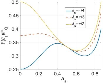
Since our scheme only measures the auxiliary states with successful post-selection, the Fisher information of the whole process satisfies ${F}_{Q}\left({\theta }_{s}\right)={p}_{f}F\left({\theta }_{s}\right)+{F}_{{p}_{f}}.$ The successful probability of post-selection is independent of the phase ${\theta }_{s},$ so ${F}_{{p}_{f}}=0,$ then we can get ${F}_{Q}\left({\theta }_{s}\right)={p}_{f}F\left({\theta }_{s}\right).$ When the dephasing does not occur, the quantum Fisher information about the target phase ${\theta }_{s}$ by using the scheme in figure 2 is $Q\left({\theta }_{s}\right)=4{a}_{s}^{2}\left(1-{a}_{s}^{2}\right).$ As shown in figure 9, the ratio ${F}_{Q}\left({\theta }_{s}\right)/Q\left({\theta }_{s}\right)$ is always greater than 0, which means that we can still obtain the target phase even if a dephasing situation occurs.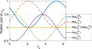
Figure 7. Matrix elements of the auxiliary qubit after dephasing as a function of the imposed phase shift ${\delta }_{s}.$ Here, p = 0 and ${\theta }_{s}=\pi /3.$ |
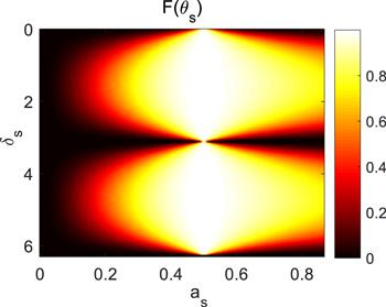
Figure 8. Quantum Fisher information of auxiliary states after complete dephasing. It can be seen that the Fisher information of the auxiliary state after the H gate operation is not 0. At this time, we can perform a Pauli measurement on the auxiliary state to obtain the target phase. |
Figure 9. The ratio ${F}_{Q}\left({\theta }_{s}\right)/Q\left({\theta }_{s}\right)$ as a function of the probability amplitude ${a}_{s}.$ Although the quantum Fisher information of this scheme cannot be fully recovered, its Fisher information is always greater than 0 at least, which means that we can still obtain the target phase by projection measurement at this time. |
5. Conclusion
In this work, a direct measurement scheme of quantum states without the assistance of pointer states is proposed. Compared with previous weak-value-based schemes, it simplifies the practical experimental procedures while eliminating the need for a post-selection process. This scheme can obtain arbitrary specific elements of the state density matrix. Meanwhile, when we consider the dephasing in the target quantum state, we modify the scheme, and the modified scheme is still applicable to the dephasing situation. This scheme is easy to be expanded and integrated, laying the foundation for the realization of direct quantum tomography in integrated quantum chips.
Acknowledgments
This research was supported by National Natural Science Foundation of China (62075049) and (61701139).
Disclosures
The authors declare no conflicts of interest.