


1. Introduction
Dimensionality is a fundamental aspect of quantum many-body physics. In particular, investigating quantum fluctuations along the crossovers from three dimensions (3D) to quasi-2D or 1D can set up the bridge between the theoretical low-D models and the actually 3D physics world. For instance, Tomonaga–Luttinger liquid [1] exists in 1D, while the high-Tc superconductivity [2] and magic-angle graphene [3–5] occur in 2D; these exotic phenomena at various low dimensions have stimulated ongoing interests and efforts to explore how the dimensionality affects quantum many-body systems using Bose–Einstein condensates (BEC). With state-of-the-art technology, quasi-1D [6] and quasi-2D [7, 8] BECs can be realized by controlling the depth of optical lattices. Along this research line, numerous tight-confinement schemes [9–17] have been proposed where BECs can undergo dimensional crossovers directly from 3D to 2D or 1D (i.e. 3D-2D or 3D-1D crossover).
These prior works have focused on single-component BECs, where the low-lying excitation is just the density excitation. To our best knowledge, however, a further account of the spin degrees of freedom (d.o.f.), a key ingredient playing out in modern physics, is still lacking in the study of dimensional crossovers. Compared to the single-component case, quantum gases with spin d.o.f can display novel phenomenology through the emergence of both the density and spin-density excitations. Therefore, we anticipate the spin d.o.f. greatly enriches dimensional-crossover physics.
Here, we theoretically investigate the dimensional crossovers in a Rabi-coupled two-component BEC. Such systems have attracted great attention recently [18, 19], since they not only allow for extending the well-known Rabi problem of atom optics to the interacting systems, it turns out that the population transfer between the two levels can be described by Josephson dynamics, leading to internal Josephson effects.
In a Rabi-coupled two-component BEC, compared to the one-component case, the additional spin d.o.f introduces two new aspects. The first is associated with the existence of inter- and intra-spin interactions, whose interplay can significantly influence quantum fluctuations. In particular, [20] has predicted that a mixture of repulsive quantum gases in 3D with finely-tuned mutual attraction may lead to the self-bound states stabilized by quantum fluctuations, known as the quantum droplet [20–22]. In low dimensions, where quantum fluctuations are enhanced, the quantum droplet states exhibit properties distinct from the 3D case at equilibrium [23] and near equilibrium [24]. The second aspect is associated with the Rabi coupling between the two internal levels, which makes the relative phase excitations gapped. Very recently, [19] has experimentally measured the beyond-mean-field equation of state in a coherently coupled two-component BEC. Thus, it is interesting and desired to study the dimensional crossovers based on the Rabi coupled two-component BEC.
Specifically, we study the quantum fluctuation of an optically trapped Rabi-coupled two-component BEC along the dimensional crossover. Using the Green function approach and the Bogoliubov approximation, we calculate the ground-state energy and the quantum depletion. Our results show that the lattice induces a characteristic 3D to quasi-2D or quasi-1D crossover in the behavior of ground-state energy. We analyze how the combined effects of spin d.o.f and dimensionality affect the quantum fluctuation.
The paper is structured as follows. In section 2 , we introduce our general theoretical model, based on which we study the dimensional crossover from 3D to quasi-low-dimensional cases in the following two sections. In section 3 , we first study a 3D BEC trapped in a 1D optical lattice and investigate the dimensional crossover behavior from 3D to quasi-2D by increasing the lattice depth. Then, we study 3D BEC trapped in a 2D optical lattice, and investigate the dimensional crossover from 3D to quasi-1D in the ground state energy and quantum depletion. We conclude with a summary in section 4 .
2. Hamiltonian of an optically trapped two-component BEC
We consider a Rabi-coupled two-component BEC in 3D, with two internal states labelled by σ = a, b, which is trapped in a d-dimensional (d = 1 or 2) optical lattice. At zero temperature, the system can be well described by the N-body Hamiltonian [22, 19, 18, 25]1 ), the lattice potential takes the form
$\begin{eqnarray}\begin{array}{rcl}H-\mu \hat{N} & = & \int {\rm{d}}{\boldsymbol{r}}\displaystyle \sum _{\sigma =a,b}{\hat{{\rm{\Psi }}}}_{\sigma }^{\dagger }({\boldsymbol{r}})\left[-\displaystyle \frac{{{\hslash }}^{2}{{\rm{\nabla }}}^{2}}{2m}-\mu +{V}_{\mathrm{opt}}({\boldsymbol{r}})\right]{\hat{{\rm{\Psi }}}}_{\sigma }({\boldsymbol{r}})\\ & + & \int {\rm{d}}{\boldsymbol{r}}\displaystyle \sum _{\{\sigma ,{\sigma }^{{\prime} }\}}\left\{\Space{0ex}{1.7ex}{0ex}{\hat{{\rm{\Psi }}}}_{\sigma }^{\dagger }({\boldsymbol{r}}){{\rm{\Pi }}}_{\sigma {\sigma }^{{\prime} }}{\hat{{\rm{\Psi }}}}_{{\sigma }^{{\prime} }}({\boldsymbol{r}})\right.\\ & + & \left.\displaystyle \frac{{g}_{\sigma {\sigma }^{{\prime} }}}{2}{\hat{{\rm{\Psi }}}}_{\sigma }^{\dagger }({\boldsymbol{r}}){\hat{{\rm{\Psi }}}}_{{\sigma }^{{\prime} }}^{\dagger }({\boldsymbol{r}}){\hat{{\rm{\Psi }}}}_{\sigma }({\boldsymbol{r}}){\hat{{\rm{\Psi }}}}_{{\sigma }^{{\prime} }}({\boldsymbol{r}})\right\}.\end{array}\end{eqnarray}$
Here ${\hat{{\rm{\Psi }}}}_{\sigma }({\boldsymbol{r}})$ is the annihilation Bose-field operator, m is the mass, μ is the chemical potential, and $\hat{N}=\int {\rm{d}}{\boldsymbol{r}}[{\hat{{\rm{\Psi }}}}_{a}^{\dagger }({\boldsymbol{r}}){{\rm{\Psi }}}_{a}({\boldsymbol{r}})\,+{\hat{{\rm{\Psi }}}}_{b}^{\dagger }({\boldsymbol{r}}){{\rm{\Psi }}}_{b}({\boldsymbol{r}})]$ is the number operator. In the second line, Π = ℏΩσx/2 is the single-particle Hamiltonian written in terms of Pauli matrices. In the third line, ${g}_{\sigma {\sigma }^{{\prime} }}=4\pi {{\hslash }}^{2}{a}_{\sigma {\sigma }^{{\prime} }}/m$ denote the intra-atomic (gaa = gbb = g) and inter-atomic (gab) coupling constants, respectively, with the scattering length ${a}_{\sigma {\sigma }^{{\prime} }}$. In equation ( $\begin{eqnarray}{V}_{\mathrm{opt}}({\boldsymbol{r}})={V}_{\mathrm{opt}}\times {E}_{R}\displaystyle \sum _{i=1}^{d}{\sin }^{2}({q}_{B}{x}_{i}).\end{eqnarray}$
Here x1 = x (x2 = y) denotes the space coordinate. The lattice strength Vopt is in units of the recoil energy of ${E}_{R}={{\hslash }}^{2}{q}_{B}^{2}/2m$, with qB the Bragg momentum and lB = π/qB the lattice period.We assume Vopt are relatively large (Vopt ≥ 5), so that the size of the interband gap Egap is larger than the chemical potential μ, i.e. Egap ≫ μ. Meanwhile, we assume the overlap of the wave functions of two consecutive wells is still sufficient to ensure full coherence. By this assumption [9–12], we restrict ourselves to the lowest Bloch band, where the physics is governed by the ratio between the chemical potential μ and the bandwidth of 4dJ, with J the tunneling rates between neighboring wells. In general, for 4dJ ≫ μ, the system retains an anisotropic 3D behavior, whereas for 4dJ ≃ μ, the system crossovers to the (3−d) dimension. In the limit of 4dJ ≪ μ, the model system can be treated as (3−d)-dimensional.
Following [9–12], we treat our system within the tight-binding approximation. Restricting ourselves only to the lowest Bloch band in the trapped direction, we write the wavefunction in terms of the Wannier functions as ${\prod }_{i=1}^{d}{\phi }_{{k}_{{x}_{i}}}({x}_{i})$, with ${\phi }_{{k}_{{x}_{i}}}({x}_{i})={\sum }_{j}{{\rm{e}}}^{{\rm{i}}{{jk}}_{{x}_{i}}{x}_{i}}w({x}_{i}-{{jl}}_{B})$. Here, $w({x}_{i})=\exp \left[-{x}_{i}^{2}/2{\xi }^{2}\right]/{\pi }^{1/4}{\xi }^{1/2}$, for i = 1, 2 (x1 = x, x2 = y), and ${l}_{B}/\xi =\pi {V}_{\mathrm{opt}}^{1/4}\exp \left(-1/4\sqrt{{V}_{\mathrm{opt}}}\right)$. We note that further account of the beyond-lowest-Bloch-band transverse modes goes beyond the scope of this work.
Following [10, 12], we expand the field operators in Hamiltonian (1 ) as ${\hat{{\rm{\Psi }}}}_{a}({\boldsymbol{r}})={\sum }_{{\boldsymbol{k}}}{\sum }_{i=1}^{d}{\hat{a}}_{{\boldsymbol{k}}}{{\rm{e}}}^{-{\rm{i}}{k}_{z}z}{\phi }_{{k}_{{x}_{i}}}({x}_{i})$ and ${\hat{{\rm{\Psi }}}}_{b}({\boldsymbol{r}})={\sum }_{{\boldsymbol{k}}}{\sum }_{i=1}^{d}{\hat{b}}_{{\boldsymbol{k}}}{{\rm{e}}}^{-{\rm{i}}{k}_{z}z}{\phi }_{{k}_{{x}_{i}}}({x}_{i})$. We obtain3 ) in the presence of d-dimensional optical lattice acquires two important differences: (i) the interaction coupling constants have been renormalized by the optical lattice as $\tilde{g}={C}^{d}g$ and ${\tilde{g}}_{{ab}}={C}^{d}{g}_{{ab}}$ with $C=\sqrt{\pi /2}/({q}_{B}\xi )$. This is because the tight optical lattice effectively increases the repulsive interactions. (ii) Instead of taking the quadratic form as in the free space, the kinetic energy ${\varepsilon }_{{\boldsymbol{k}}}^{0}$ along the confinement direction becomes
$\begin{eqnarray}\begin{array}{rcl}\hat{H}-\mu \hat{N} & = & \displaystyle \sum _{{\boldsymbol{k}}}\left({\varepsilon }_{{\boldsymbol{k}}}^{0}-\mu \right)\left({\hat{a}}_{{\boldsymbol{k}}}^{\dagger }{\hat{a}}_{{\boldsymbol{k}}}+{\hat{b}}_{{\boldsymbol{k}}}^{\dagger }{\hat{b}}_{{\boldsymbol{k}}}\right)\\ & + & \displaystyle \frac{{\hslash }{\rm{\Omega }}}{2}\displaystyle \sum _{{\boldsymbol{k}}}\left({\hat{a}}_{{\boldsymbol{k}}}^{\dagger }{\hat{b}}_{{\boldsymbol{k}}}+{\hat{b}}_{{\boldsymbol{k}}}^{\dagger }{\hat{a}}_{{\boldsymbol{k}}}\right)\\ & + & \displaystyle \frac{\tilde{g}}{2V}\displaystyle \sum _{{{\boldsymbol{k}}}_{1}{{\boldsymbol{k}}}_{2}{\boldsymbol{q}}}\left({\hat{a}}_{{{\boldsymbol{k}}}_{1}+{\boldsymbol{q}}}^{\dagger }{\hat{a}}_{{{\boldsymbol{k}}}_{2}-{\boldsymbol{q}}}^{\dagger }{\hat{a}}_{{{\boldsymbol{k}}}_{2}}{\hat{a}}_{{{\boldsymbol{k}}}_{1}}+{\hat{b}}_{{{\boldsymbol{k}}}_{1}+{\boldsymbol{q}}}^{\dagger }{\hat{b}}_{{{\boldsymbol{k}}}_{2}-{\boldsymbol{q}}}^{\dagger }{\hat{b}}_{{{\boldsymbol{k}}}_{2}}{\hat{b}}_{{{\boldsymbol{k}}}_{1}}\right)\\ & + & \displaystyle \frac{{\tilde{g}}_{{ab}}}{V}\displaystyle \sum _{{{\boldsymbol{k}}}_{1}{{\boldsymbol{k}}}_{2}{\boldsymbol{q}}}{\hat{a}}_{{{\boldsymbol{k}}}_{1}+{\boldsymbol{q}}}^{\dagger }{\hat{b}}_{{{\boldsymbol{k}}}_{2}-{\boldsymbol{q}}}^{\dagger }{\hat{b}}_{{{\boldsymbol{k}}}_{2}}{\hat{a}}_{{{\boldsymbol{k}}}_{1}},\end{array}\end{eqnarray}$
with V the system volume. Compared to the Hamiltonian [19] of a Rabi-coupled two-component BEC without optical confinement, Hamiltonian ( $\begin{eqnarray}{\varepsilon }_{{\boldsymbol{k}}}^{0}=2J\sum _{i=1}^{d}\left[1-\cos \left(\displaystyle \frac{{{\boldsymbol{k}}}_{i}\pi }{{q}_{B}}\right)\right]+\sum _{i=1}^{3-d}\displaystyle \frac{{{\hslash }}^{2}{{\boldsymbol{k}}}_{i}^{2}}{2m},\end{eqnarray}$
with the tunneling rate $\begin{eqnarray}\begin{array}{rcl}J & = & \int {{\rm{d}}}^{d}{\boldsymbol{x}}\displaystyle \sum _{i=1}^{d}{w}^{* }({x}_{i})\left(-\displaystyle \frac{{{\hslash }}^{2}}{2m}\displaystyle \frac{{\partial }^{2}}{\partial {x}_{i}^{2}}+{V}_{\mathrm{opt}}({\boldsymbol{r}})\right)\\ & & \times \,w({x}_{i}+{l}_{B}).\end{array}\end{eqnarray}$
Following [19], we treat Hamiltonian (3 ) within the framework of Bogoliubov approximation. This consists of separating the dominant contribution from the condensates (i.e. ${a}_{{\boldsymbol{k}}=0}=\sqrt{{n}_{a}^{0}}$ and ${b}_{{\boldsymbol{k}}=0}=\sqrt{{n}_{b}^{0}}{{\rm{e}}}^{{\rm{i}}\phi }$) from the other modes (i.e. ${\hat{a}}_{{\boldsymbol{k}}\ne 0}$ and ${\hat{b}}_{{\boldsymbol{k}}\ne 0}$). At the zeroth order, we obtain the mean-field energy ${E}_{\mathrm{MF}}=\tfrac{1}{2}g[{\left({n}_{a}^{0}\right)}^{2}+{\left({n}_{b}^{0}\right)}^{2}]+{g}_{{ab}}{n}_{a}^{0}{n}_{b}^{0}\,+\sqrt{{n}_{a}^{0}{n}_{b}^{0}}{\hslash }{\rm{\Omega }}\cos \phi -\mu ({n}_{a}^{0}+{n}_{b}^{0})$. The mean-field energy EMF can be minimized for φ = π. Depending on the interplay between intra- and inter-spin interactions, the ground state is different. When gab < g + 2ℏΩ/n0, the ground state is a neutral ground sate described by ${n}_{a}^{0}={n}_{b}^{0}={n}_{0}/2$. When gab > g + 2ℏΩ/n0, the ground state is polarized, with ${n}_{a}^{0}-{n}_{b}^{0}={n}_{0}\sqrt{1-{\left(2{\rm{\Omega }}/(g-{g}_{{ab}}){n}_{0}\right)}^{2}}$.
We are interested in the neutral ground state with ${n}_{a}^{0}={n}_{b}^{0}={n}_{0}/2$. The transition from the spin-unpolarized to the spin-polarized phases, which occurs at a critical interaction constant $\tilde{g}={\tilde{g}}_{{ab}}+2{\hslash }{\rm{\Omega }}/{n}_{0}$, is beyond the scope of the current work. Applying the Bogoliubov theory [9–12, 15, 19] to equation (3 ) under the stated conditions, we obtain an effective Hamiltonian6 ).
$\begin{eqnarray}\begin{array}{rcl}\hat{H}-\mu \hat{N} & = & {E}_{\mathrm{MF}}+\displaystyle \sum _{{\boldsymbol{k}}\ne 0}\Space{0ex}{0.25ex}{0ex}[{\varepsilon }_{{\boldsymbol{k}}}^{0}-\mu +\tilde{g}n+\displaystyle \frac{{\tilde{g}}_{{ab}}n}{2}\Space{0ex}{0.25ex}{0ex}]\\ & & \times \,({\hat{a}}_{{\boldsymbol{k}}}^{\dagger }{\hat{a}}_{{\boldsymbol{k}}}+{\hat{b}}_{{\boldsymbol{k}}}^{\dagger }{\hat{b}}_{{\boldsymbol{k}}})\\ & + & \displaystyle \frac{\tilde{g}n}{4}\displaystyle \sum _{{\boldsymbol{k}}\ne 0}({\hat{a}}_{{\boldsymbol{k}}}^{\dagger }{\hat{a}}_{-{\boldsymbol{k}}}^{\dagger }+{\hat{a}}_{{\boldsymbol{k}}}{a}_{-{\boldsymbol{k}}}+{\hat{b}}_{{\boldsymbol{k}}}^{\dagger }{\hat{b}}_{-{\boldsymbol{k}}}^{\dagger }+{\hat{b}}_{{\boldsymbol{k}}}{\hat{b}}_{-{\boldsymbol{k}}})\\ & + & \Space{0ex}{0.25ex}{0ex}(\displaystyle \frac{{\hslash }{\rm{\Omega }}}{2}-\displaystyle \frac{{\tilde{g}}_{{ab}}n}{2}\Space{0ex}{0.25ex}{0ex})\displaystyle \sum _{{\boldsymbol{k}}\ne 0}({a}_{{\boldsymbol{k}}}^{\dagger }{\hat{b}}_{{\boldsymbol{k}}}+{\hat{b}}_{{\boldsymbol{k}}}^{\dagger }{\hat{a}}_{{\boldsymbol{k}}})\\ & - & \displaystyle \frac{{\tilde{g}}_{{ab}}n}{2}\displaystyle \sum _{{\boldsymbol{k}}\ne 0}({\hat{a}}_{{\boldsymbol{k}}}^{\dagger }{\hat{b}}_{-{\boldsymbol{k}}}^{\dagger }+{\hat{b}}_{{\boldsymbol{k}}}{\hat{a}}_{-{\boldsymbol{k}}}),\end{array}\end{eqnarray}$
with $\mu =(\tilde{g}+{\tilde{g}}_{{ab}})n/2-{\hslash }{\rm{\Omega }}/2$ and n the total density. Our subsequent studies of dimensional crossover will be based on Hamiltonian (We aim to derive the beyond-mean-field ground state energy Eg and the quantum depletion (N − N0)/N of an optically-trapped Bose gas. To this end, we exploit the approach developed by Hugenholtz and Pines [26]. Using the single-particle Green function [27], we have7 ) and (8 ), G(k, ω) is the Fourier transform of the Green function $G({\boldsymbol{k}},t-{t}^{{\prime} })=-{\rm{i}}\left\langle T{\hat{a}}_{{\boldsymbol{k}}}(t){\hat{a}}_{{\boldsymbol{k}}}^{\dagger }({t}^{{\prime} })\right\rangle $ in the time domain, with T denoting the chronological product. Following the standard procedures [26, 28], we obtain7 ) and (8 ) provide the central equations for our subsequent study of the dimensional crossover of the optically-trapped Rabi-coupled two-component Bose gas.
$\begin{eqnarray}\begin{array}{rcl}\displaystyle \frac{{E}_{g}}{V} & = & {E}_{\mathrm{MF}}+\mathop{\mathrm{lim}}\limits_{t\to 0-}\displaystyle \frac{{\rm{i}}{q}_{B}^{d}}{{\left(2\pi \right)}^{3}{\pi }^{d}}\int {\rm{d}}{k}_{z}{{\rm{d}}}^{d}{\boldsymbol{k}}\\ & & \times \,\int \displaystyle \frac{{\rm{d}}\omega }{2\pi {\rm{i}}}{{\rm{e}}}^{-{\rm{i}}\omega t}E({\boldsymbol{k}})G({\boldsymbol{k}},\omega ),\end{array}\end{eqnarray}$
where E(k) is the excitation energy, and $\begin{eqnarray}\displaystyle \frac{N-{N}_{0}}{N}=\mathop{\mathrm{lim}}\limits_{t\to 0-}\displaystyle \frac{{\rm{i}}{q}_{B}^{d}}{{\left(2\pi \right)}^{4}{\pi }^{d}n}\int {\rm{d}}{k}_{z}{{\rm{d}}}^{d}{\boldsymbol{k}}\int {\rm{d}}\omega {{\rm{e}}}^{-{\rm{i}}\omega t}G({\boldsymbol{k}},\omega ).\end{eqnarray}$
In equations ( $\begin{eqnarray}\begin{array}{rcl}G\left({\boldsymbol{k}},\omega \right) & = & \displaystyle \frac{1}{2}\displaystyle \frac{{\hslash }\omega +{\varepsilon }_{{\boldsymbol{k}}}^{0}+\tfrac{\tilde{g}+{\tilde{g}}_{{ab}}}{2}n}{{\left({\hslash }\omega \right)}^{2}-{\varepsilon }_{1}^{2}({\boldsymbol{k}})+{\rm{i}}0}\\ & + & \displaystyle \frac{1}{2}\displaystyle \frac{{\hslash }\omega +{\varepsilon }_{{\boldsymbol{k}}}^{0}+{\hslash }{\rm{\Omega }}+\tfrac{\tilde{g}-{\tilde{g}}_{{ab}}}{2}n}{{\left({\hslash }\omega \right)}^{2}-{\varepsilon }_{2}^{2}({\boldsymbol{k}})+{\rm{i}}0}\\ & = & \displaystyle \frac{1}{2}{G}_{1}({\boldsymbol{k}},\omega )+\displaystyle \frac{1}{2}{G}_{2}({\boldsymbol{k}},\omega ),\end{array}\end{eqnarray}$
with $\begin{eqnarray}{\varepsilon }_{1}({\boldsymbol{k}})=\sqrt{{\varepsilon }_{{\boldsymbol{k}}}^{0}[{\varepsilon }_{{\boldsymbol{k}}}^{0}+(\tilde{g}+{\tilde{g}}_{{ab}})n]},\end{eqnarray}$
$\begin{eqnarray}{\varepsilon }_{2}({\boldsymbol{k}})=\sqrt{({\varepsilon }_{{\boldsymbol{k}}}^{0}+{\hslash }{\rm{\Omega }})[{\varepsilon }_{{\boldsymbol{k}}}^{0}+{\hslash }{\rm{\Omega }}+(\tilde{g}-{\tilde{g}}_{{ab}})n]}.\end{eqnarray}$
Equations (3. Dimensional crossovers of an optically-trapped Rabi-coupled two-component BEC
According to equations (7 ) and (8 ), the spin d.o.f. introduces two new ingredients compared to the scalar BEC. Namely, the beyond-mean-field ground state energy Eg and the quantum depletion (N − N0)/N now depend on, firstly, the $\tilde{g}$ and ${\tilde{g}}_{{ab}}$ associated with the spin-dependent interactions, and secondly, the Rabi-frequency ℏΩ. In particular, the Rabi-coupling ∝ℏΩ between the two components gives rise to phase correlations between the two components, in contrast to the density-density correlations coming from the interspecies interaction $\tilde{g}$. Note that such coupling can be implemented via a two-photon (Raman) process or direct coupling between the two internal states.
To identify the respective roles of the spin-dependent interaction and the Rabi coupling on the dimensional crossover, we devise two scenarios. In scenario (i), we take $\tilde{g}={\tilde{g}}_{{ab}}$ and investigate how the Rabi-coupling affects the dimensional crossover. In scenario (ii), we turn off the Rabi coupling, i.e. ℏΩ = 0, and study how the dimensional crossover is affected by the spin-dependent interaction quantified by ${\tilde{g}}_{{ab}}=\lambda \tilde{g}$ with λ ≠ 1.
We shall first consider a 1D optical lattice along the x-direction and study the dimensional crossover from 3D to quasi-2D in section 3.1 . Then, we consider a 2D optical lattice along both x- and y- directions and study the dimensional crossover from 3D to quasi-1D in section 3.2 .
3.1. Dimensional crossover from 3D to quasi-2D
In this section, we study a Rabi-coupled two-component Bose gas in a 1D optical lattice ${V}_{\mathrm{opt}}(x)={V}_{\mathrm{opt}}\times {E}_{R}{\sin }^{2}({q}_{B}x)$ in the x-direction; atoms are unconfined in the y−z plane. In this case, the single-particle energy in equation (9 ) can be written as ${\varepsilon }_{{\boldsymbol{k}}}^{0}=2J[1-\cos ({k}_{x}{l}_{B})]+{{\hslash }}^{2}({k}_{y}^{2}+{k}_{z}^{2})/2m$.
We begin with scenario (i), where $\tilde{g}={\tilde{g}}_{{ab}}$ and ℏΩ ≠ 0. To explicitly construct an analytic solution, we exploit the fact that typical experimental mixtures of hyperfine states of bosonic alkali atoms are near the boundary of phase separation instability, namely the coupling constants satisfy the inequality $\tilde{g}-{\tilde{g}}_{{ab}}\ll \tilde{g}$ in order to avoid the phase separation. For the two hyperfine states of Na, for example, one has $(\tilde{g}-{\tilde{g}}_{{ab}})/\tilde{g}\approx 0.07$. For $\tilde{g}={\tilde{g}}_{{ab}}$, the Green function (9 ) can be simplified as
$\begin{eqnarray}\begin{array}{rcl}G\left({\boldsymbol{k}},\omega \right) & = & \displaystyle \frac{1}{2}\displaystyle \frac{{\hslash }\omega +{\varepsilon }_{{\boldsymbol{k}}}^{0}+\tilde{g}n}{{\left({\hslash }\omega \right)}^{2}-{\varepsilon }_{1}^{2}({\boldsymbol{k}})+{\rm{i}}0}\\ & & +\displaystyle \frac{1}{2}\displaystyle \frac{1}{{\hslash }\omega -{\varepsilon }_{{\boldsymbol{k}}}^{0}-{\hslash }{\rm{\Omega }}+{\rm{i}}0}.\end{array}\end{eqnarray}$
Plugging equation (12 ) into equations (7 ) and (8 ), we derive the quantum depletions in each component, i.e. ${n}_{1\mathrm{ex}}=\langle {\sum }_{{\boldsymbol{k}}\ne 0}{\hat{a}}_{{\boldsymbol{k}}}^{\dagger }{\hat{a}}_{{\boldsymbol{k}}}\rangle $ and ${n}_{2\mathrm{ex}}=\langle {\sum }_{{\boldsymbol{k}}\ne 0}{\hat{b}}_{{\boldsymbol{k}}}^{\dagger }{\hat{b}}_{{\boldsymbol{k}}}\rangle $, with n1ex = n2ex, as well as the beyond-mean-field ground state energy Eg/V. After straightforward but tedious calculation, we obtain
$\begin{eqnarray}\begin{array}{rcl}{n}_{1\mathrm{ex}} & = & \mathop{\mathrm{lim}}\limits_{t\to -0}\displaystyle \frac{1}{{\left(2\pi \right)}^{2}}\int {{\rm{d}}}^{2}{\boldsymbol{k}}\displaystyle \frac{1}{2\pi {l}_{B}}{\int }_{-\pi }^{\pi }{\rm{d}}{k}_{x}\displaystyle \frac{{\rm{i}}}{2\pi }\\ & & \times \,{\int }_{C}{\rm{d}}\omega {{\rm{e}}}^{-{\rm{i}}\omega t}G({\boldsymbol{k}},\omega )\\ & = & \displaystyle \frac{m\tilde{g}n}{4{\pi }^{2}{{\hslash }}^{2}{l}_{B}}{\rm{\Delta }}(s),\end{array}\end{eqnarray}$
and $\begin{eqnarray}\begin{array}{rcl}\displaystyle \frac{{E}_{g}}{V} & = & {E}_{\mathrm{MF}}-2\mathop{\mathrm{lim}}\limits_{t\to -0}\displaystyle \frac{1}{{\left(2\pi \right)}^{2}}\int {{\rm{d}}}^{2}{\boldsymbol{k}}\displaystyle \frac{1}{2\pi {l}_{B}}\\ & & \times \,{\int }_{-\pi }^{\pi }{\rm{d}}{k}_{x}\displaystyle \frac{{\rm{i}}}{2\pi }{\int }_{C}{\rm{d}}\omega {{\rm{e}}}^{-{\rm{i}}\omega t}{\varepsilon }_{1}({\boldsymbol{k}})\displaystyle \frac{1}{2}{G}_{1}({\boldsymbol{k}},\omega )\\ & = & {M}_{\mathrm{MF}}+\displaystyle \frac{m{\tilde{g}}^{2}{n}^{2}}{4\pi {{\hslash }}^{2}{l}_{B}}{\rm{\Gamma }}\left(s\right),\end{array}\end{eqnarray}$
with $s=2J/\tilde{g}n$ and $\begin{eqnarray}{\rm{\Delta }}(s)=\left(s+1\right)\arctan \displaystyle \frac{1}{\sqrt{s}}-\sqrt{s},\end{eqnarray}$
$\begin{eqnarray}{\rm{\Gamma }}(s)={\int }_{-\pi }^{\pi }\displaystyle \frac{{\rm{d}}{k}_{x}}{2\pi }{\int }_{s(1-\cos {k}_{x})}^{\infty }{\rm{d}}\eta \left(\displaystyle \frac{1}{2\eta }-\eta -1+\sqrt{\eta \left(\eta +2\right)}\right).\end{eqnarray}$
It turns out that the Rabi term ℏΩ does not explicitly enter the expressions of quantum depletions and beyond-mean-field ground state energy. Such surprising results can be understood as follows. Mathematically, the ℏΩ only appears in the second term of the Green function (12 ). It can be shown that the corresponding integrals in equations (13 ) and (14 ) yield the zero value, i.e. ${\int }_{C}{\rm{d}}\omega /({\hslash }\omega -{\varepsilon }_{{\bf{k}}}^{0}-{\hslash }{\rm{\Omega }}+{\rm{i}}0)=0$ where C denotes the contour of integration. As a result, ℏΩ disappears in equations (13 ) and (14 ). From the physical angle, the second term of equation (12 ) shows that the energy level ${\varepsilon }_{2}({\boldsymbol{k}})={\varepsilon }_{{\boldsymbol{k}}}^{0}+{\hslash }{\rm{\Omega }}$ acts only as the transition state such as ${\hat{a}}_{{\boldsymbol{k}}}$ to ${\hat{b}}_{{\boldsymbol{k}}}^{\dagger }$ and there are no particles really occupying this spectrum. Therefore, the second term of equation (12 ) does not contribute to equations (13 ) and (14 ).
Next, we turn to scenario (ii) where ℏΩ = 0 and show how the spin-dependent interactions, i.e. ${\tilde{g}}_{{ab}}=\lambda \tilde{g}$ with λ ≠ 1, can affect the dimensional crossover. In this case, the Green function (9 ) becomes17 ) contribute to the quantum fluctuations, different from scenario (i) where only the first term of equation (12 ) contributes. The quantum depletions n1ex = n2ex and the beyond-mean-field energy Eg/V can be calculated by directly plugging equation (17 ) into equations (7 ) and (8 ). We find
$\begin{eqnarray}\begin{array}{rcl}G\left({\boldsymbol{k}},\omega \right) & = & \displaystyle \frac{1}{2}\displaystyle \frac{{\hslash }\omega +{\varepsilon }_{{\boldsymbol{k}}}^{0}+\tfrac{\tilde{g}+{\tilde{g}}_{{ab}}}{2}n}{{\left({\hslash }\omega \right)}^{2}-{\varepsilon }_{1}^{2}({\boldsymbol{k}})+{\rm{i}}0}\\ & & +\displaystyle \frac{1}{2}\displaystyle \frac{{\hslash }\omega +{\varepsilon }_{{\boldsymbol{k}}}^{0}+\tfrac{\tilde{g}-{\tilde{g}}_{{ab}}}{2}n}{{\left({\hslash }\omega \right)}^{2}-{\varepsilon }_{2}^{2}({\boldsymbol{k}})+{\rm{i}}0}.\end{array}\end{eqnarray}$
Obviously, both the two terms in equation ( $\begin{eqnarray}\begin{array}{rcl}{n}_{1\mathrm{ex}} & = & \mathop{\mathrm{lim}}\limits_{t\to -0}\displaystyle \frac{1}{{\left(2\pi \right)}^{2}}\int {{\rm{d}}}^{2}{\boldsymbol{k}}\displaystyle \frac{1}{2\pi {l}_{B}}{\int }_{-\pi }^{\pi }{\rm{d}}{k}_{x}\displaystyle \frac{{\rm{i}}}{2\pi }{\int }_{C}{\rm{d}}\omega {{\rm{e}}}^{-{\rm{i}}\omega t}G({\boldsymbol{k}},\omega )\\ & = & \displaystyle \frac{{mn}}{8{\pi }^{2}{{\hslash }}^{2}{l}_{B}}\left[\left(\tilde{g}+{\tilde{g}}_{{ab}}\right){\rm{\Delta }}({\tilde{s}}_{1})+\left(\tilde{g}-{\tilde{g}}_{{ab}}\right){\rm{\Delta }}({\tilde{s}}_{2})\right]\\ & = & \displaystyle \frac{{mn}\tilde{g}}{8{\pi }^{2}{{\hslash }}^{2}{l}_{B}}\left[\left.(1+\lambda ){\rm{\Delta }}\Space{0ex}{1.0ex}{0ex}(\displaystyle \frac{2}{1+\lambda }s\right)\right.\\ & & \left.+(1-\lambda ){\rm{\Delta }}\Space{0ex}{1.0ex}{0ex}(\displaystyle \frac{2}{1-\lambda }s\Space{0ex}{1.0ex}{0ex})\right]\\ & = & \displaystyle \frac{{mn}\tilde{g}}{8{\pi }^{2}{{\hslash }}^{2}{l}_{B}}\delta (s),\end{array}\end{eqnarray}$
and $\begin{eqnarray}\begin{array}{rcl}\displaystyle \frac{{E}_{g}}{V} & = & {E}_{\mathrm{MF}}-2\mathop{\mathrm{lim}}\limits_{t\to -0}\displaystyle \frac{1}{{\left(2\pi \right)}^{2}}\int {{\rm{d}}}^{2}{\boldsymbol{k}}\displaystyle \frac{1}{2\pi {l}_{B}}{\int }_{-\pi }^{\pi }{\rm{d}}{k}_{x}\displaystyle \frac{{\rm{i}}}{2\pi }\\ & & \times \,{\int }_{C}{\rm{d}}\omega {{\rm{e}}}^{-{\rm{i}}\omega t}({\varepsilon }_{1}({\boldsymbol{k}})\displaystyle \frac{1}{2}{G}_{1}({\boldsymbol{k}},\omega )+{\varepsilon }_{2}({\boldsymbol{k}})\displaystyle \frac{1}{2}{G}_{2}({\boldsymbol{k}},\omega ))\\ & = & {E}_{\mathrm{MF}}+\displaystyle \frac{{{mn}}^{2}}{16\pi {{\hslash }}^{2}{l}_{B}}\left[{\left(\tilde{g}+{\tilde{g}}_{{ab}}\right)}^{2}{\rm{\Gamma }}({\tilde{s}}_{1})+{\left(\tilde{g}-{\tilde{g}}_{{ab}}\right)}^{2}{\rm{\Gamma }}({\tilde{s}}_{2})\right]\\ & = & {E}_{\mathrm{MF}}+\displaystyle \frac{{{mn}}^{2}{\tilde{g}}^{2}}{16\pi {{\hslash }}^{2}{l}_{B}}\left[{\left(1+\lambda \right)}^{2}{\rm{\Gamma }}\Space{0ex}{1.0ex}{0ex}(\displaystyle \frac{2}{1+\lambda }s\Space{0ex}{1.0ex}{0ex})\right.\\ & & \left.+{\left(1-\lambda \right)}^{2}{\rm{\Gamma }}\Space{0ex}{1.0ex}{0ex}(\displaystyle \frac{2}{1-\lambda }s\Space{0ex}{1.0ex}{0ex})\right]\\ & = & {E}_{\mathrm{MF}}+\displaystyle \frac{{{mn}}^{2}{\tilde{g}}^{2}}{16\pi {{\hslash }}^{2}{l}_{B}}\gamma (s),\end{array}\end{eqnarray}$
with ${\tilde{s}}_{\mathrm{1,2}}=4J/(\tilde{g}\pm {\tilde{g}}_{{ab}})n$.Now, we are ready to study the quantum fluctuations along the dimensional crossover. In the asymptotic limit $s,{\tilde{s}}_{\mathrm{1,2}}\gg 1$, equations (13 ), (14 ), (18 ), and (19 ) recover the well-known results in 3D [29]. Specifically, the quantum depletions in equations (13 ) or (18 ) asymptotically approach ${n}_{1\mathrm{ex}}^{3D}\simeq \tfrac{1}{6{\pi }^{2}{{\hslash }}^{2}}\sqrt{\tfrac{{m}^{* }}{m}}{\left({mn}\tilde{g}\right)}^{3/2}$ or ${n}_{1\mathrm{ex}}^{3D}\simeq \tfrac{1}{6{\pi }^{2}{{\hslash }}^{2}}\sqrt{\tfrac{{m}^{* }}{m}}[{\left({mn}(\tilde{g}+{\tilde{g}}_{{ab}})/2\right)}^{3/2}+{\left({mn}(\tilde{g}-{\tilde{g}}_{{ab}})/2\right)}^{3/2}]$ with the effective mass ${m}^{* }={{\hslash }}^{2}/2{{Jl}}_{B}^{2}$ in the 3D limit where $\arctan {s}^{-\tfrac{1}{2}}\approx {s}^{-\tfrac{1}{2}}-{s}^{-\tfrac{3}{2}}/3$. Similarly, in equations (14 ) and (19 ), we find ${\rm{\Gamma }}(s)\simeq 32/15\pi \sqrt{s}$, so that the asymptotic beyond-mean-field ground state energy is ${E}_{g}^{3D}/V={E}_{\mathrm{MF}}+\tfrac{8}{15}\sqrt{\tfrac{{m}^{* }}{m}}\tfrac{{m}^{3/2}}{{\pi }^{2}{{\hslash }}^{3}}{\left(\tilde{g}n\right)}^{5/2}$ and ${E}_{g}^{3D}/V={E}_{\mathrm{MF}}\,+\tfrac{8}{15}\sqrt{\tfrac{{m}^{* }}{m}}\tfrac{{m}^{3/2}}{{\pi }^{2}{{\hslash }}^{3}}\left[{\left(\tfrac{\tilde{g}+{\tilde{g}}_{{ab}}}{2}n\right)}^{5/2}+{\left(\tfrac{\tilde{g}-{\tilde{g}}_{{ab}}}{2}n\right)}^{5/2}\right]$, respectively. In the limit s ≪ 1, on the other hand, the function Δ(s) in equation (15 ) saturates to the value of π/2 and equation (13 ) asymptotically approaches $\tfrac{m\tilde{g}n}{8\pi {{\hslash }}^{2}{l}_{B}}$ which is the known result for the 2D quantum depletion.
To visualize the behavior of quantum fluctuations in the entire crossover regimes, we focus on equations (18 ) and (19 ), as ℏΩ does not explicitly play a role as stated previously. In figure 1(a), we show the scaling function γ(s) and its asymptotic behavior with λ = 0.95. In the limit s ≫ 1, the asymptotic law is $\gamma (s)\simeq 32{\left(1+\lambda \right)}^{2}/(15\pi \sqrt{s})$. in figure 1(b) we show the scaling function δ(s) and its asymptotic behavior with λ = 0.95. For vanishing s, δ(s) saturates to π, no matter what the value of λ is. In the limit s ≫ 1, the asymptotic law is $\delta (s)\simeq 2(1+\lambda )/(3\sqrt{s})$.
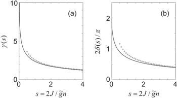
Figure 1. (a) Scaling function γ(s) (solid line) in equation ( |
Note that we do not consider the effect of the confinement-induced resonance (CIR) [30, 31] on the coupling constant $\tilde{g}$. This is because the basic physics of CIR can be understood in the language of Feshbach resonance [32], where the scattering open channel and closed channels are, respectively, represented by the ground-state transverse mode and the other transverse modes along the tight-confinement dimensions. Within the tight-binding approximation, however, the ultracold atoms are frozen in the states of the lowest Bloch band and can not be excited into the other transverse modes. Thus the effect of CIR on $\tilde{g}$ can be safely ignored due to the absence of closed channels [30–32].
3.2. Dimensional crossover from 3D to quasi-1D
In this section, we study the dimensional crossover from 3D to quasi-1D of a Rabi-coupled two-component Bose gas trapped into a 2D optical lattice as ${V}_{\mathrm{opt}}({\boldsymbol{r}})\,={V}_{\mathrm{opt}}{E}_{R}[{\sin }^{2}({q}_{B}x)+{\sin }^{2}({q}_{B}y)]$. In this case, the dispersion relation of the single particle becomes ${\varepsilon }_{{\boldsymbol{k}}}^{0}=\tfrac{{{\hslash }}^{2}{k}_{z}^{2}}{2m}\,+2J[2-\cos {k}_{x}-\cos {k}_{y}]$.
Previously, we have stated that the Rabi-coupling constant of ℏΩ does not enter the analytical expressions of quantum depletion and beyond-mean-field ground state energy. We found that this statement still hold in the case of the dimensional crossover from 3D to 1D. As such, we only consider scenario (ii) where ${\tilde{g}}_{{ab}}=\lambda \tilde{g}$ and Ω = 0. We find
$\begin{eqnarray}\begin{array}{rcl}{n}_{1\mathrm{ex}}={n}_{1\mathrm{ex}} & = & \mathop{\mathrm{lim}}\limits_{t\to -0}\displaystyle \frac{1}{2\pi }\int {\rm{d}}{k}_{z}\displaystyle \frac{1}{{\left(2\pi {l}_{B}\right)}^{2}}{\int }_{-\pi }^{\pi }{{\rm{d}}}^{2}{\boldsymbol{k}}\displaystyle \frac{{\rm{i}}}{2\pi }\\ & & \times \,{\int }_{C}{\rm{d}}\omega {{\rm{e}}}^{-{\rm{i}}\omega t}\Space{0ex}{0.25ex}{0ex}(\displaystyle \frac{1}{2}{G}_{1}({\boldsymbol{k}},\omega \Space{0ex}{0.25ex}{0ex})+\displaystyle \frac{1}{2}{G}_{2}({\boldsymbol{k}},\omega )\Space{0ex}{1.0ex}{0ex})\\ & = & \displaystyle \frac{\sqrt{{mn}\tilde{g}}}{8\pi {\hslash }{l}_{B}^{2}}\left[\sqrt{1+\lambda }H\Space{0ex}{0.25ex}{0ex}(\displaystyle \frac{2}{1+\lambda }s\Space{0ex}{0.25ex}{0ex})\right.\\ & & \left.+\sqrt{1-\lambda }H\Space{0ex}{0.25ex}{0ex}(\displaystyle \frac{2}{1-\lambda }s\Space{0ex}{0.25ex}{0ex})\right]\\ & = & \displaystyle \frac{\sqrt{{mn}\tilde{g}}}{8\pi {\hslash }{l}_{B}^{2}}h(s),\end{array}\end{eqnarray}$
and $\begin{eqnarray}\begin{array}{rcl}\displaystyle \frac{{E}_{g}}{V} & = & {E}_{\mathrm{MF}}-2\mathop{\mathrm{lim}}\limits_{t\to -0}\displaystyle \frac{1}{2\pi }\int {\rm{d}}{k}_{z}\displaystyle \frac{1}{{\left(2\pi {l}_{B}\right)}^{2}}{\int }_{-\pi }^{\pi }{{\rm{d}}}^{2}{\boldsymbol{k}}\displaystyle \frac{{\rm{i}}}{2\pi }\\ & & \times \,{\int }_{C}{\rm{d}}\omega {{\rm{e}}}^{-{\rm{i}}\omega t}\left({\varepsilon }_{1}\left({\boldsymbol{k}}\right)\displaystyle \frac{1}{2}{G}_{1}\left({\boldsymbol{k}},\omega \right)\right.\\ & & \left.+{\varepsilon }_{2}\left({\boldsymbol{k}}\right)\displaystyle \frac{1}{2}{G}_{2}\left({\boldsymbol{k}},\omega \right)\right)\\ & = & {E}_{\mathrm{MF}}-\displaystyle \frac{\sqrt{{mn}\tilde{g}}n\tilde{g}}{8\pi {\hslash }{l}_{B}^{2}}\left[{\left(1+\lambda \right)}^{3/2}F\left(\displaystyle \frac{2}{1+\lambda }s\right)\right.\\ & & \left.+{\left(1-\lambda \right)}^{3/2}F\left(\displaystyle \frac{2}{1-\lambda }s\right)\right]\\ & = & {E}_{\mathrm{MF}}-\displaystyle \frac{\sqrt{{mn}\tilde{g}}n\tilde{g}}{8\pi {\hslash }{l}_{B}^{2}}f(s),\end{array}\end{eqnarray}$
with $\begin{eqnarray}\begin{array}{rcl}H(s) & = & {\int }_{-\pi }^{\pi }\displaystyle \frac{{{\rm{d}}}^{2}k}{{\left(2\pi \right)}^{2}}{\int }_{s\left[2-\cos {k}_{x}-\cos {k}_{y}\right]}^{\infty }{\rm{d}}\eta \\ & & \times \,\displaystyle \frac{1}{\sqrt{\eta -s\left(2-\cos {k}_{x}-\cos {k}_{y}\right)}}\left[\displaystyle \frac{\eta +1}{\sqrt{\eta (\eta +2)}}-1\right],\end{array}\end{eqnarray}$
and $\begin{eqnarray}\begin{array}{rcl}F(s) & = & \displaystyle \frac{\pi }{2\sqrt{s}}{\int }_{-\pi }^{\pi }\displaystyle \frac{{{\rm{d}}}^{2}{\boldsymbol{k}}}{{\left(2\pi \right)}^{2}}\displaystyle \frac{1}{\sqrt{2-\cos {k}_{x}-\cos {k}_{y}}}\\ & & \times \,{}_{2}{F}_{1}\left[\displaystyle \frac{1}{2},\displaystyle \frac{3}{2},3,\displaystyle \frac{-2}{s\left[2-\cos {k}_{x}-\cos {k}_{y}\right]}\right].\end{array}\end{eqnarray}$
Now, we study the dimensional crossover from 3D toward 1D based on equations (20 ) and (21 ). In the limit of s ≫ 1, we find equations (20 ) and (21 ) recover the well-known 3D results [29], namely the system retains an anisotropic 3D behavior. Specifically, for s ≫ 1, the asymptotic law is $F(s)\simeq [1.43/\sqrt{s}-16\sqrt{2}/(15\pi s)]$ in equation (23 ) and $H(s)\simeq 4/(3\pi \sqrt{2}s)$ in equation (22 ). It follows from equations (20 ) and (21 ) that we asymptotically obtain ${n}_{1\mathrm{ex}}^{3D}\simeq \tfrac{1}{6{\pi }^{2}{{\hslash }}^{2}}\sqrt{\tfrac{{m}^{* }}{m}}[{\left({mn}(\tilde{g}+{\tilde{g}}_{{ab}})/2\right)}^{3/2}+{\left({mn}(\tilde{g}-{\tilde{g}}_{{ab}})/2\right)}^{3/2}]$ and ${E}_{g}^{3D}/V={E}_{\mathrm{MF}}+\tfrac{8}{15}\sqrt{\tfrac{{m}^{* }}{m}}\tfrac{{m}^{3/2}}{{\pi }^{2}{{\hslash }}^{3}} $ $\left[{\left(\tfrac{\tilde{g}+{\tilde{g}}_{{ab}}}{2}n\right)}^{5/2}+{\left(\tfrac{\tilde{g}-{\tilde{g}}_{{ab}}}{2}n\right)}^{5/2}\right]$.
In the opposite limit s ≪ 1, $H(s)\simeq 4/(3\pi \sqrt{2}s)$ in equation (22 ) is divergent like $H(s)\simeq -\mathrm{ln}(2.7s)/\sqrt{2}$, so the quantum depletion in equation (20 ) diverges. It implies that in the absence of tunneling, no real Bose–Einstein condensation exists, which agrees with the general theorems in one dimension. Meanwhile, the F(s) in equation (23 ) saturates to the value $4\sqrt{2}/3$. In this limit, we can neglect the Bloch dispersion and equation (21 ) approaches asymptotically to the ground state energy of a 1D Bose gas as ${E}_{g}^{1D}/V\,={E}_{\mathrm{MF}}-\tfrac{2}{3\pi }\sqrt{m}\left[{\left(\tfrac{\tilde{g}+{\tilde{g}}_{{ab}}}{2}{n}_{1D}\right)}^{3/2}+{\left(\tfrac{\tilde{g}-{\tilde{g}}_{{ab}}}{2}{n}_{1D}\right)}^{3/2}\right]$ with the effective 1D density of ${n}_{1D}={{nl}}_{B}^{2}$.
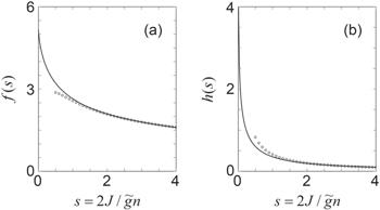
In figure 2, we plot the functions h(s) in equation (20 ) and f(s) in equation (21 ). Their asymptotic behaviors are also shown. Thus we conclude that equations (20 ) and (21 ) provide the analytical expressions of quantum depletion and beyond-mean-field ground state along the 3D-1D dimensional crossover.
Figure 2. (a) Scaling function $f(s)={\left(1+\lambda \right)}^{3/2}F(\tfrac{2}{1+\lambda }s)\,+{\left(1-\lambda \right)}^{3/2}F(\tfrac{2}{1-\lambda }s)$ (solid line) in equation ( |
4. Discussion and conclusion
The calculations of this work are based on the mean-field Bogoliubov theory, which can be justified as a posteriori by estimating the quantum depletion [9]. Note that there is no experimental study of quantum depletion of Rabi-coupled two-component BEC. In what follows, we plan to adopt the experimental parameters of one-component BEC to estimate the quantum depletion in equations (13 ) and (20 ). In more detail, the experimental work [33, 34] has shown that the Bogoliubov theory provides a semiquantitative description for an optically-trapped one-component BEC even in the case of the quantum depletions being in excess of 50%. It is supposed that such a statement is still valid for an optically-trapped Rabi-coupled two-component. We limit ourselves into the case of $\tilde{g}={\tilde{g}}_{{ab}}=g=4\pi {{\hslash }}^{2}{a}_{3D}/m$ in order to simplifying the estimation. For a uniform BEC, the quantum depletion is $(N-{N}_{0})/N=8/3\sqrt{{{na}}_{3D}^{2}}$ and the Bogoliubov approximation is valid provided $\sqrt{{{na}}_{3D}^{2}}$ is small. For an optically-trapped Rabi-coupled two-component BEC in the regime $\tilde{g}={\tilde{g}}_{{ab}}=g$, the above quantum depletion is modified qualitatively as $(8{m}^{* }/3m)\sqrt{n{\tilde{a}}_{3D}/\pi }$ with m* the effective mass. Considering typical experimental parameters as in [9], this modification remains small. For an optically-trapped Rabi-coupled two-component Bose gas along the dimensional crossovers, we take the parameters in the experiment in [35]: n = 3 × 1013 cm−3, lB = 430 nm, a3D = 5.4 nm, and lB/ξ ∼ 1. The corresponding quantum depletion is evaluated as (N − N0)/N ∼ 0.0036 × δ(s) or h(s) with δ(s) and h(s) shown in figures 1(b) and 2(b) respectively. It is clear that the quantum depletion (N − N0)/N < 20%, and therefore, the Bogoliubov approximation is valid in the sprit of [33, 34].
Summarizing, we have investigated a 3D Rabi-coupled two-component BEC trapped in a 1D and 2D optical lattice, respectively. We have analytically derived the ground-state energy and the quantum depletion. Our results show the 3D to quasi-2D or quasi-1D crossovers in the behavior of quantum fluctuations. The underlying physics involves the interplay of three quantities: the strength of the optical lattice, the interaction between bosonic atoms, and the spin d.o.f. All these quantities are experimentally controllable at present. Notably, the state-of-the-art technology allows the depth of an optical lattice to be arbitrarily tuned by changing the laser intensities, enabling realizations of quasi-1D [6] and quasi-2D [7, 8] BECs. [36] has demonstrated fast control of the interatomic interactions by coherently coupling two atomic states with intra- and interstate scattering lengths almost at will. Furthermore, the beyond-mean-field equation of the state of a Rabi-coupled two-component has been experimentally measured by [19]. Therefore, the phenomena discussed in this paper are supposed to be observable within the current experimental capabilities. Directly observing such dimensional effects on the novel quantum phases in a Rabi-coupled two-component BEC, e.g. quantum droplet [20, 23], would present an important step in revealing the interplay between dimensionality, quantum fluctuations and spin d.o.f in quasi-low dimensions.