


1. Introduction
The Heisenberg–Kitaev (HK) model on various lattices such as triangular, kagome, pyrochlore, hyperkagome and fcc lattices has attracted a lot of attention because there are frustrations from the competing exchange couplings coexisting with the geometric frustration of the underlying lattices, which may lead to exotic states such as quantum spin liquid and topological orders [1–11]. The studies were also connected to real materials, such as the layered honeycomb materials α-RuCl3, Na2IrO3 and α-Ir2IrO3, the three-dimensional (3D) honeycomb material (β-γ)-Li2IrO3, and the iridium oxides with triangular lattices [12–42].
The rare-earth-based kagome lattice (KL) compounds ${\mathrm{Mg}}_{2}{\mathrm{RE}}_{3}{\mathrm{Sb}}_{3}{{\rm{O}}}_{14}$ $(\mathrm{RE}=\mathrm{Gd},\ \mathrm{Er})$ and $(\mathrm{RE}=\mathrm{Nd})$ have q = 0, 120° order and canted ferromagnetic (CFM) order [43, 44], respectively. These compounds, except for $\mathrm{RE}=\mathrm{Gd}$, have an effective spin with S = 1/2 on the KL [45]. Since the exchange couplings between the nearest-neighbor (NN) spins are anisotropic, Morita et al studied the ground state of the classical and quantum spin HK model with anisotropic bond-dependent Kitaev interactions on the KL [46]. Interestingly, the ground state has the same type q = 0, 120° order and CFM order as those observed in the compounds. In the theoretical phase diagram, the CFM order resides in a continuous parameter region, and there is no phase change across special parameter points, such as the Kitaev ferromagnetic (KFM) point, the ferromagnetic (FM) point and its dual FM point. However, a ground state property cannot distinguish a system with or without topological nontrivial excitations and related phase transitions. The non-coplanar CFM order naturally has nonzero scalar spin chirality, which will provide a vector potential for magnons [47]. Then one may wonder if there are topological magnon excitations and the related thermal Hall effect in the system. Furthermore, whether is it possible for a topological phase transition of magnon excitations to happen on the continuous CFM ground state.
Here, we study the topological magnon excitations and related thermal Hall conductivity in the HK model on the KL with CFM order. In the CFM order, the solid angle spanned by the three spins in a unit cell changes continuously with the model parameter [48]. However, the continuous CFM phase can be divided into two regions related by the Klein duality, with the self dual KFM point as their boundary [48], and we are surprised to find that the scalar spin chirality which is intrinsic in the CFM order changes sign across the KFM point. This leads to the opposite Chern numbers of corresponding magnon bands in the two regions, and also the sign change of the magnon thermal Hall conductivity.
This paper is organized as follows. In section 2 , we revisit the CFM phase in the model and investigate the scalar spin chirality. In section 3 , we present the magnon band structures and discuss their topological properties. In section 4 , we show the transverse thermal Hall conductivity with sign change phenomena. Finally, a summary is given in section 5 .
2. Model, the CFM phase and scalar spin chirality
We first revisit the model and the CFM phase [46, 48]. Consider interacting spins that reside on the KL as shown in figure 1(a). The HK model is described by the spin Hamiltonian
$\begin{eqnarray}H=\sum _{\langle {ij}\rangle }(J{{\boldsymbol{S}}}_{i}\cdot {{\boldsymbol{S}}}_{j}+{{KS}}_{i}^{{\gamma }_{{ij}}}{S}_{j}^{{\gamma }_{{ij}}}),\end{eqnarray}$
where Si and Sj are spin S = 1/2 spins reside on the NN lattice sites, and J and K denote the Heisenberg and Kitaev exchange couplings, respectively. The Cartesian components γij equals x, y or z, depending on the bond type as shown in figure 1(a). The model can be parameterized by $\begin{eqnarray}J=\cos \psi ,\quad K=\sin \psi ,\quad \psi \in [0,2\pi ),\end{eqnarray}$
with the energy unit J2 + K2 = 1.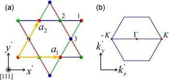
Figure 1. (a) The structure of the KL. There are three spins that reside in a primitive cell, which are denoted by red, green and blue sites. Red, green and blue bonds between NN sites (i, j) carry three distinct Kitaev couplings ${S}_{i}^{x}{S}_{j}^{x}$, ${S}_{i}^{y}{S}_{j}^{y}$ and ${S}_{i}^{x}{S}_{j}^{x}$, respectively. Meanwhile, there are isotropic Heisenberg couplings in all the NN bonds. The KL sits on the (111) plane, and we define a new 2D frame ${x}^{{\prime} }{y}^{{\prime} }$ on the KL with basis vectors a1 = (1, 0) and ${{\boldsymbol{a}}}_{2}=(1,\sqrt{3})/2$. (b) The first Brillouin zone of the KL. |
In the classical ground state phase diagram of the HK model on KL, there is a long-range ordered CFM phase for $\psi \in [\pi -\arctan (2),2\pi ]$, which has eightfold degeneracy. At the phase boundary are the classical spin liquid (CSL) state and dual CSL state corresponding to the Heisenberg point with K = 0 and its dual point, respectively. Inside the CFM phase, there are other three special points, the KFM point with J = 0, the FM point with K = 0 and its dual FM point (see figure 2(a)). There is no phase transition of the ground state across the whole CFM phase. However, we find that the collective magnon excitations on the CFM ground state do have topological phase transition at the KFM point as shown in figure 2(a). Interestingly, we can divide the CFM phase into two regions related by the Klein duality [46, 48, 49], with the self-dual KFM point as the boundary. The Klein duality preserves the form of the Hamiltonian but alter the value of the parameters J and K, and in the KL it reads
$\begin{eqnarray}\widetilde{H}=\sum _{\langle {ij}\rangle }(\widetilde{J}\,{\widetilde{{\boldsymbol{S}}}}_{i}\cdot {\widetilde{{\boldsymbol{S}}}}_{j}+\widetilde{K}{\widetilde{S}}_{i}^{{\gamma }_{{ij}}}{\widetilde{S}}_{j}^{{\gamma }_{{ij}}}),\end{eqnarray}$
where $\begin{eqnarray}\widetilde{J}=-J,\quad \widetilde{K}=2J+K,\end{eqnarray}$
and the spin operators transform to $\begin{eqnarray}{\widetilde{{\boldsymbol{S}}}}_{1}=\left(\begin{array}{c}-{S}_{1}^{x}\\ {S}_{1}^{y}\\ -{S}_{1}^{z}\end{array}\right),{\widetilde{{\boldsymbol{S}}}}_{2}=\left(\begin{array}{c}{S}_{2}^{x}\\ -{S}_{2}^{y}\\ -{S}_{2}^{z}\end{array}\right),{\widetilde{{\boldsymbol{S}}}}_{3}=\left(\begin{array}{c}{S}_{3}^{x}\\ {S}_{3}^{y}\\ {S}_{3}^{z}\end{array}\right).\end{eqnarray}$
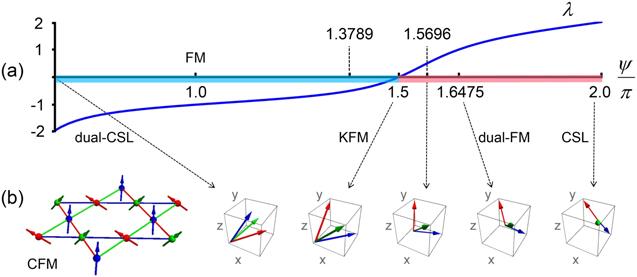
Figure 2. (a) Evolution of λ (equation ( |
The spin structure of the CFM phase can be described by the directions of the three spins in a primitive cell [48]
$\begin{eqnarray}{{\boldsymbol{S}}}_{1}=\xi S\left(\begin{array}{c}-\lambda \chi \\ \eta \\ \zeta \end{array}\right),{{\boldsymbol{S}}}_{2}=\xi S\left(\begin{array}{c}\chi \\ -\lambda \eta \\ \zeta \end{array}\right),{{\boldsymbol{S}}}_{3}=\xi S\left(\begin{array}{c}\chi \\ \eta \\ -\lambda \zeta \end{array}\right),\end{eqnarray}$
where $\xi =1/\sqrt{2+{\lambda }^{2}}$ and $\begin{eqnarray}\lambda =(\cos \psi +\sin \psi +\sqrt{5+4\cos 2\psi +\sin 2\psi })/(2\cos \psi ).\end{eqnarray}$
The eight degenerate spin orders are given by χ = ± 1, η = ± 1 and ζ = ± 1. The magnon excitations of the eight different spin orders have the same band structures, however different wave functions and therefore different topological properties. Here, we study the order given by χ = η = ζ = 1, which is the same as the one observed in experiment [44], as shown in figure 2(b).Since the three spins in a primitive cell are non-coplanar in the CFM order, there is intrinsically non-zero scalar spin chirality. In the spin order with χ = η = ζ = 1, the scalar spin chirality isA ) and its dual one. On the left side of the KFM point, the solid angle Ω spanned by spins S1,2,3 is smaller than its dual one $\widetilde{{\rm{\Omega }}}$ (see figure 3(b)), which is spanned by the dual spins ${\widetilde{{\boldsymbol{S}}}}_{\mathrm{1,2,3}}$, and the chirality for magnons is S1 · (S2 × S3). However, the situation is opposite in the right side of the KFM point, and now the chirality for magnons will be ${\widetilde{{\boldsymbol{S}}}}_{1}\cdot ({\widetilde{{\boldsymbol{S}}}}_{2}\times {\widetilde{{\boldsymbol{S}}}}_{3})$.
$\begin{eqnarray}{{\boldsymbol{S}}}_{1}\cdot ({{\boldsymbol{S}}}_{2}\times {{\boldsymbol{S}}}_{3}){/S}^{3}=\displaystyle \frac{-{\lambda }^{3}+3\lambda +2}{{\left({\lambda }^{2}+2\right)}^{3/2}},\end{eqnarray}$
and its dual one is $\begin{eqnarray}{\widetilde{{\boldsymbol{S}}}}_{1}\cdot ({\widetilde{{\boldsymbol{S}}}}_{2}\times {\widetilde{{\boldsymbol{S}}}}_{3}){/S}^{3}=\displaystyle \frac{-{\lambda }^{3}+3\lambda -2}{{\left({\lambda }^{2}+2\right)}^{3/2}}.\end{eqnarray}$
It turns out that the chirality is always positive except at the FM and CSL points, where it vanishes. Oppositely, the dual chirality is always negative and vanishes at the dual FM and dual CSL points, as shown in figure 3(a). Here we are surprised to find that the scalar spin chirality for the magnons changes sign at the KFM point, where it jumps from the original chirality to its dual one. We attribute it to the relative size of the corresponding solid angle (see appendix 
Figure 3. (a) Evolutions of the scalar spin chirality (equation ( |
The scalar spin chirality can provides a vector potential for magnons, which will lead to topological magnons and thermal Hall effect, as previous studies on ferromagnets with Dzyaloshinskii–Moriya (DM) interaction induced vector potential [50–55]. The more interesting thing here is the scalar spin chirality changes sign across the KFM point. This will lead to the opposite Chern numbers of corresponding magnon bands in the two dual regions, and also the sign change of the magnon thermal Hall conductivity, as we show in the next sections.
3. Band structure and topological magnons
Now we turn to study the collective magnon excitations on the CFM order with χ = η = ζ = 1. Starting from the Hamiltonian (1 ), after the Holstein–Primakoff (HP) [56] and Fourier transformations, we get the magnon Hamiltonian matrix $h({{\boldsymbol{k}}}^{{\prime} })$ (see appendix B ). Then after diagonalizing ${I}_{-}h({{\boldsymbol{k}}}^{{\prime} })$, we get three magnon bands. The magnon bands are gapped in all the CFM phase, except at the CSL, dual CSL, FM, dual FM and KFM points as shown in the top panel of figure 4. Due to the same form of the Hamiltonian, the band structures are the same for any pair of dual points, except for the energy scale. At the FM and dual FM points, the magnon bands are the same as the isotropic Heisenberg model on KL [53]. At the CSL and dual CSL points, there are zero energy flat bands, which means the magnon modes now can excite without energy cost. Moreover, the possibilities for the excited magnon modes with different ${{\boldsymbol{k}}}^{{\prime} }$ are the same, and this will lead to the breakdown of the long-range order. Here the breakdown of the CFM order gives the CSL phase. At the KFM point, there is also a flat band, however with finite energy. Hence, to excite the flat band modes now will cost energy, and the CFM order is protected by the energy gap.
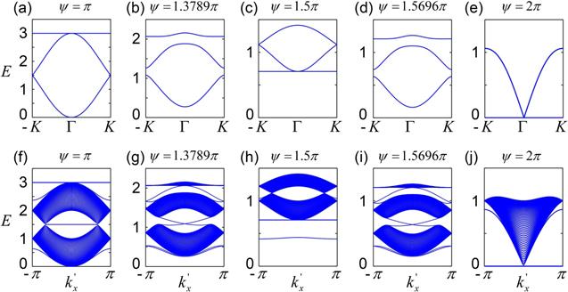
Figure 4. Top panel: magnon bands of the CFM order at the (a) FM point, (c) KFM point, (e) CSL point, and (b) and (d) a pair of dual points. The magnon bands are gapped in all the CFM phase, except at the CSL, dual CSL, FM, dual FM and KFM points. The points (b) ψ = 1.3789π and (d) ψ = 1.5696π also denoted in figure 2(a) are a pair of dual points, and their band structures are the same except for the energy scale. The bands in (b) carry Chern numbers 1, 0, −1, while they are −1, 0, 1 in (d). Bottom panel: the corresponding magnon bands in a strip geometry. There are in-gap edge modes for the gapped band structures, which are promised by the nonzero Chern numbers of the corresponding bulk bands. |
Though the band structures of the dual points are the same, the wave functions and topological properties are not necessarily the same. To show the topological property of the gapped magnon bands, we calculate their Chern numbers. The Chern number of the nth band is defined by the integration of the Berry curvature over the first Brillouin zone [57]
$\begin{eqnarray}{C}_{n}=\displaystyle \frac{1}{2\pi }{\int }_{\mathrm{BZ}}{\rm{d}}{k}_{x}^{{\prime} }{\rm{d}}{k}_{y}^{{\prime} }{B}_{{k}_{x}^{{\prime} }{k}_{y}^{{\prime} }}^{n},\end{eqnarray}$
with $\begin{eqnarray}{B}_{{k}_{x}^{{\prime} }{k}_{y}^{{\prime} }}^{n}={\rm{i}}\sum _{{n}^{{\prime} }\ne n}\displaystyle \frac{\left\langle {\phi }_{n}| \tfrac{\partial h({{\boldsymbol{k}}}^{{\prime} })}{\partial {k}_{x}^{{\prime} }}| {\phi }_{{n}^{{\prime} }}\Space{0ex}{1.0ex}{0ex}\rangle \langle {\phi }_{{n}^{{\prime} }}| \tfrac{\partial h({{\boldsymbol{k}}}^{{\prime} })}{\partial {k}_{y}^{{\prime} }}| {\phi }_{n}\rangle -\Space{0ex}{1.0ex}{0ex}({k}_{x}^{{\prime} }\leftrightarrow {k}_{y}^{{\prime} }\right)}{{\left({E}_{n}-{E}_{{n}^{{\prime} }}\right)}^{2}},\end{eqnarray}$
where En and φn are the eigenvalue and eigenvector of the nth band respectively. It turns out that the Chern numbers are (C1, C2, C3) = (1, 0, − 1) in the region $\psi \in (\pi -\arctan (2),1.5\pi )$, while they are (−1, 0, 1) in the region ψ ∈ (1.5π, 2π). This denotes a topological phase transition at the KFM point ψ = 1.5π (see figure 2(a)). We show the gapped magnon bands of a pair of dual points in figures 4(b) and (d), and their Chern numbers are opposite. As mentioned in the above section, it is the sign change of the scalar spin chirality for magnons that leads to the opposite Berry curvatures and Chern numbers of corresponding magnon bands in the two regions related by Klein duality. Due to the bulk-edge correspondence [58], the nonzero Chern numbers will promise in-gap edge modes in a strip geometry as shown in figures 4(g) and (i).4. Transverse thermal Hall conductivity with sign change
As previous studies on ferromagnets with DM interaction induced vector potential, the scalar spin chirality here can also provide a vector potential for magnons, which will lead to the magnon thermal Hall effect. Furthermore, the sign change of the chirality here will also induce the sign change of the thermal conductivity simultaneously. The transverse thermal Hall conductivity can be calculated as [59–61]
$\begin{eqnarray}{\kappa }_{{x}^{{\prime} }{y}^{{\prime} }}=\displaystyle \frac{{k}_{{\rm{B}}}^{2}T}{{\left(2\pi \right)}^{2}{\hslash }}\sum _{n}{\int }_{\mathrm{BZ}}{{c}}_{2}({\rho }_{n}){{\rm{B}}}_{{k}_{x}^{{\prime} }{k}_{y}^{{\prime} }}^{n}{\rm{d}}{k}_{x}^{{\prime} }{\rm{d}}{k}_{y}^{{\prime} },\end{eqnarray}$
with the sum running over the three bands and the integral is over the first Brillouin zone. ${\rho }_{n}=1/({\rm{\exp }}({E}_{n}/{k}_{{\rm{B}}}T)-1)$ is the Bose distribution with En as the nth eigenvalue. c2 is given by $\begin{eqnarray}{c}_{2}({\rho }_{n})=(1+{\rho }_{n}){\left(\mathrm{ln}\displaystyle \frac{1+{\rho }_{n}}{{\rho }_{n}}\right)}^{2}-{\left(\mathrm{ln}{\rho }_{n}\right)}^{2}-2{\mathrm{Li}}_{2}(-{\rho }_{n}),\end{eqnarray}$
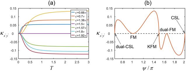
where Li2(x) is the polylogarithm function of order 2.As shown in figures 5(a) and (b), the transverse thermal conductivity for $\psi \in (\pi -\arctan (2),1.5\pi )$ is always positive, while it is always negative for ψ ∈ (1.5π, 2π). At the CSL, dual CSL, FM, dual FM and KFM points, the magnon bands are gapless, leading to vanishing thermal Hall conductivity. There is sign change of the thermal conductivity at the KFM point, and we attribute it to the sign change of the scalar spin chirality. As the chirality changes sign, the vector potential for magnons becomes opposite, and the propagating magnons will be deflected in the opposite direction, which results in the opposite transverse conductivity.
Figure 5. (a) The transverse thermal conductivity as a function of temperature for different ψ. For $\psi \in (\pi -\arctan (2),1.5\pi )$, the conductivity is always positive, while for ψ ∈ (1.5π, 2π) it is always negative. At the CSL, dual CSL, FM, dual FM and KFM points, the conductivity is always zero. (b) The transverse thermal conductivity as a function of ψ with T = 3. There is sign change at the KFM point. Here we set ℏ = kB = 1. |
The sign change of the thermal Hall conductivity is also consistent with the opposite Chern numbers of corresponding magnon bands. Consider the high temperature limit of the transverse thermal conductivity [55, 62]
$\begin{eqnarray}{\kappa }_{{x}^{{\prime} }{y}^{{\prime} }}^{\mathrm{lim}}=\mathop{\mathrm{lim}}\limits_{T\to \infty }{\kappa }_{{x}^{{\prime} }{y}^{{\prime} }}=-\displaystyle \frac{{k}_{{\rm{B}}}}{{\left(2\pi \right)}^{2}{\hslash }}\sum _{n}{\int }_{\mathrm{BZ}}{E}_{n}{B}_{{k}_{x}^{{\prime} }{k}_{y}^{{\prime} }}^{n}{\rm{d}}{k}_{x}^{{\prime} }{\rm{d}}{k}_{y}^{{\prime} },\end{eqnarray}$
it can be further simplified as $\begin{eqnarray}{\kappa }_{{x}^{{\prime} }{y}^{{\prime} }}^{\mathrm{lim}}\propto -\displaystyle \frac{{k}_{{\rm{B}}}}{{\left(2\pi \right)}^{2}{\hslash }}\sum _{n}{C}_{n}{\overline{E}}_{n},\end{eqnarray}$
where the ${{\boldsymbol{k}}}^{{\prime} }$-dependent band energy is replaced by the average ${\overline{E}}_{n}$. Then the high temperature thermal conductivity of the phase with Chern numbers (1, 0, −1) is ${\overline{E}}_{3}-{\overline{E}}_{1}$ which is positive, while the conductivity of the phase with Chern numbers (−1, 0, 1) is ${\overline{E}}_{1}-{\overline{E}}_{3}$ which is negative. Then the sign change of the chirality, the opposite Chern numbers of corresponding bands and the sign change of the thermal conductivity are consistent with each other.In the end of this section, we will discuss briefly the eight degenerate CFM spin orders. We find that the chirality of the orders with [χηζ] = [111], $[1\bar{1}\bar{1}]$, $[\bar{1}1\bar{1}]$, and $[\bar{1}\bar{1}1]$ is
$\begin{eqnarray}{{\boldsymbol{S}}}_{1}\cdot ({{\boldsymbol{S}}}_{2}\times {{\boldsymbol{S}}}_{3}){/S}^{3}=\displaystyle \frac{-{\lambda }^{3}+3\lambda +2}{{\left({\lambda }^{2}+2\right)}^{3/2}},\end{eqnarray}$
and its dual one is $\begin{eqnarray}{\widetilde{{\boldsymbol{S}}}}_{1}\cdot ({\widetilde{{\boldsymbol{S}}}}_{2}\times {\widetilde{{\boldsymbol{S}}}}_{3}){/S}^{3}=\displaystyle \frac{-{\lambda }^{3}+3\lambda -2}{{\left({\lambda }^{2}+2\right)}^{3/2}}.\end{eqnarray}$
However, the chirality of the orders $[\bar{1}\bar{1}\bar{1}]$, $[\bar{1}11]$, $[1\bar{1}1]$, and $[11\bar{1}]$ are opposite $\begin{eqnarray}{{\boldsymbol{S}}}_{1}\cdot ({{\boldsymbol{S}}}_{2}\times {{\boldsymbol{S}}}_{3}){/S}^{3}=\displaystyle \frac{{\lambda }^{3}-3\lambda -2}{{\left({\lambda }^{2}+2\right)}^{3/2}},\end{eqnarray}$
$\begin{eqnarray}{\widetilde{{\boldsymbol{S}}}}_{1}\cdot ({\widetilde{{\boldsymbol{S}}}}_{2}\times {\widetilde{{\boldsymbol{S}}}}_{3}){/S}^{3}=\displaystyle \frac{{\lambda }^{3}-3\lambda +2}{{\left({\lambda }^{2}+2\right)}^{3/2}}.\end{eqnarray}$
Besides, the solid angles Ω and $\widetilde{{\rm{\Omega }}}$ keep the same for all eight orders. This suggests that the Chern numbers of the magnon bands and the sign of the thermal Hall conductivity are the same for the orders [111], $[1\bar{1}\bar{1}]$, $[\bar{1}1\bar{1}]$, and $[\bar{1}\bar{1}1]$, while they are opposite to that of the orders $[\bar{1}\bar{1}\bar{1}]$, $[\bar{1}11]$, $[1\bar{1}1]$, and $[11\bar{1}]$.5. Summary
We have studied the topological magnon excitations and related thermal Hall conductivity in the HK model on the KL with CFM order. The CFM phase can be divided into two regions related by the Klein duality [46, 48, 49], with the self dual KFM point as their boundary. We find that the scalar spin chirality, which is intrinsic in the CFM order, changes sign across the KFM point. This leads to the opposite Chern numbers of corresponding magnon bands in the two regions, and also the sign change of the magnon thermal Hall conductivity. Moreover, we have checked that for the coplanar q = 0, 120° order [46] the magnon bands are always gapless, and there is no thermal Hall conductivity. Interestingly, the rare-earth-based KL compounds ${\mathrm{Mg}}_{2}{\mathrm{RE}}_{3}{\mathrm{Sb}}_{3}{{\rm{O}}}_{14}$ $(\mathrm{RE}=\mathrm{Gd},\ \mathrm{Er})$ and $(\mathrm{RE}=\mathrm{Nd})$ have the same q = 0, 120° order and CFM order [43, 44], respectively. Though the chiral edge modes are difficult to measure in an experiment, the sign structure of the thermal conductivity is more accessible [63]. Therefore, the study of the topological magnons and related thermal Hall conductivity here will contribute to the understanding of related compounds.
Acknowledgments
We thank Changle Liu for helpful discussions. This work was supported by the National Natural Science Foundation of China (Grant NO. 12 104 407) and the Natural Science Foundation of Zhejiang Province (Grant NO. LQ20A040004).
Appendix A. Solid angle of the three spins
The solid angle Ω spanned by the three spins in a primitive cell can be calculated as
$\begin{eqnarray}\tan \left(\displaystyle \frac{{\rm{\Omega }}}{4}\right)=\sqrt{\tan \left(\displaystyle \frac{s}{2}\right)\tan \left(\displaystyle \frac{s-\alpha }{2}\right)\tan \left(\displaystyle \frac{s-\beta }{2}\right)\tan \left(\displaystyle \frac{s-\gamma }{2}\right)},\end{eqnarray}$
where $s=\tfrac{1}{2}(\alpha +\beta +\gamma )$, and α, β and γ are the angle between spins S1,2, S2,3 and S3,1 respectively. The solid angle $\widetilde{{\rm{\Omega }}}$ spanned by the dual spins ${\widetilde{{\boldsymbol{S}}}}_{\mathrm{1,2,3}}$ has the same definition.Appendix B. Magnon Hamiltonian matrix
We denote the directions of spins Si=1,2,3 by their polar angles θ1,2,3 and azimuthal angles φ1,2,3 in the global frame. The HP transformation for a spin in its local frame reads1 ) and then do the Fourier transformation, we get the quadratic Hamiltonian in momentum space
$\begin{eqnarray}{S}_{x}^{0}=\displaystyle \frac{\sqrt{2S}}{2}(a+{a}^{\dagger }),\end{eqnarray}$
$\begin{eqnarray}{S}_{y}^{0}=\displaystyle \frac{\sqrt{2S}}{2{\rm{i}}}(a-{a}^{\dagger }),\end{eqnarray}$
$\begin{eqnarray}{S}_{z}^{0}=S-{a}^{\dagger }a,\end{eqnarray}$
where a† and a are the magnon creation and annihilation operators respectively, which obey the boson commutation rules. Then by multiplying a rotation matrix we get the HP transformation for spin Si in the global frame $\begin{eqnarray}\left(\begin{array}{c}{S}_{{ix}}\\ {S}_{{iy}}\\ {S}_{{iz}}\end{array}\right)=\left(\begin{array}{ccc}\cos {\theta }_{i}\cos {\phi }_{i} & -\sin {\phi }_{i} & \sin {\theta }_{i}\cos {\phi }_{i}\\ \cos {\theta }_{i}\sin {\phi }_{i} & \cos {\phi }_{i} & \sin {\theta }_{i}\sin {\phi }_{i}\\ -\sin {\theta }_{i} & 0 & \cos {\theta }_{i}\end{array}\right)\,\left(\begin{array}{c}{S}_{{ix}}^{0}\\ {S}_{{iy}}^{0}\\ {S}_{{iz}}^{0}\end{array}\right).\end{eqnarray}$
Substituting Six,y,z into the Hamiltonian ( $\begin{eqnarray}H=\displaystyle \frac{1}{2}\sum _{{{\boldsymbol{k}}}^{{\prime} }}{{\rm{\Psi }}}_{{{\boldsymbol{k}}}^{{\prime} }}^{\dagger }h({{\boldsymbol{k}}}^{{\prime} }){{\rm{\Psi }}}_{{{\boldsymbol{k}}}^{{\prime} }},\end{eqnarray}$
where ${{\rm{\Psi }}}_{{{\boldsymbol{k}}}^{{\prime} }}^{\dagger }=({a}_{1{{\boldsymbol{k}}}^{{\prime} }}^{\dagger },{a}_{2{{\boldsymbol{k}}}^{{\prime} }}^{\dagger },{a}_{3{{\boldsymbol{k}}}^{{\prime} }}^{\dagger },{a}_{1-{{\boldsymbol{k}}}^{{\prime} }},{a}_{2-{{\boldsymbol{k}}}^{{\prime} }},{a}_{3-{{\boldsymbol{k}}}^{{\prime} }})$. The magnon Hamiltonian matrix is $\begin{eqnarray}h({{\boldsymbol{k}}}^{{\prime} })=\left(\begin{array}{cc}{A}_{{{\boldsymbol{k}}}^{{\prime} }} & {B}_{{{\boldsymbol{k}}}^{{\prime} }}^{\dagger }\\ {B}_{{{\boldsymbol{k}}}^{{\prime} }} & {A}_{{{\boldsymbol{k}}}^{{\prime} }}^{* }\end{array}\right)S,\end{eqnarray}$
with ${A}_{{{\boldsymbol{k}}}^{{\prime} }}$ and ${B}_{{{\boldsymbol{k}}}^{{\prime} }}$ 3 × 3 matrices. Their elements are as follows $\begin{eqnarray}{A}_{11}=-2J({c}_{z}+{e}_{z})-2K({c}_{8}+{e}_{7}),\end{eqnarray}$
$\begin{eqnarray}{A}_{22}=-2J({c}_{z}+{d}_{z})-2K({c}_{8}+{d}_{6}),\end{eqnarray}$
$\begin{eqnarray}{A}_{33}=-2J({d}_{z}+{e}_{z})-2K({d}_{6}+{e}_{7}),\end{eqnarray}$
$\begin{eqnarray}{A}_{12}=[J({c}_{x}+{c}_{y}-{\rm{i}}{c}_{{xy}}+{\rm{i}}{c}_{{yx}})+{{Kc}}_{3}]\cos {{\boldsymbol{k}}}^{{\prime} }\cdot {{\boldsymbol{\delta }}}_{1},\end{eqnarray}$
$\begin{eqnarray}{A}_{21}={A}_{12}^{* },\end{eqnarray}$
$\begin{eqnarray}\begin{array}{rcl}{A}_{13} & = & [J({e}_{x}+{e}_{y}+{\rm{i}}{e}_{{xy}}-{\rm{i}}{e}_{{yx}})\\ & & +K({e}_{2}+{e}_{5}+{\rm{i}}{e}_{10}-{\rm{i}}{e}_{12})]\cos {{\boldsymbol{k}}}^{{\prime} }\cdot {{\boldsymbol{\delta }}}_{3},\end{array}\end{eqnarray}$
$\begin{eqnarray}{A}_{31}={A}_{13}^{* },\end{eqnarray}$
$\begin{eqnarray}\begin{array}{rcl}{A}_{23} & = & [J({d}_{x}+{d}_{y}-{\rm{i}}{d}_{{xy}}+{\rm{i}}{d}_{{yx}})\\ & & +K({d}_{1}+{d}_{4}-{\rm{i}}{d}_{9}+{\rm{i}}{d}_{11})]\cos {{\boldsymbol{k}}}^{{\prime} }\cdot {{\boldsymbol{\delta }}}_{2},\end{array}\end{eqnarray}$
$\begin{eqnarray}{A}_{32}={A}_{23}^{* },\end{eqnarray}$
$\begin{eqnarray}{B}_{12}={B}_{21}=[J({c}_{x}-{c}_{y}-{\rm{i}}{c}_{{xy}}-{\rm{i}}{c}_{{yx}})+{{Kc}}_{3}]\cos {{\boldsymbol{k}}}^{{\prime} }\cdot {{\boldsymbol{\delta }}}_{1},\end{eqnarray}$
$\begin{eqnarray}\begin{array}{rcl}{B}_{13} & = & {B}_{31}=[J({e}_{x}-{e}_{y}-{\rm{i}}{e}_{{xy}}-{\rm{i}}{e}_{{yx}})\\ & & +K({e}_{2}-{e}_{5}-{\rm{i}}{e}_{10}-{\rm{i}}{e}_{12})]\cos {{\boldsymbol{k}}}^{{\prime} }\cdot {{\boldsymbol{\delta }}}_{3},\end{array}\end{eqnarray}$
$\begin{eqnarray}\begin{array}{rcl}{B}_{23} & = & {B}_{32}=[J({d}_{x}-{d}_{y}-{\rm{i}}{d}_{{xy}}-{\rm{i}}{d}_{{yx}})\\ & & +K({d}_{1}-{d}_{4}-{\rm{i}}{d}_{9}-{\rm{i}}{d}_{11})]\cos {{\boldsymbol{k}}}^{{\prime} }\cdot {{\boldsymbol{\delta }}}_{2},\end{array}\end{eqnarray}$
$\begin{eqnarray}{B}_{11}={B}_{22}={B}_{33}=0,\end{eqnarray}$
where $\begin{eqnarray}{c}_{1}=\cos {\theta }_{1}\cos {\phi }_{1}\cos {\theta }_{2}\cos {\phi }_{2},\end{eqnarray}$
$\begin{eqnarray}{c}_{2}=\cos {\theta }_{1}\sin {\phi }_{1}\cos {\theta }_{2}\sin {\phi }_{2},\end{eqnarray}$
$\begin{eqnarray}{c}_{3}=\sin {\theta }_{1}\sin {\theta }_{2},\end{eqnarray}$
$\begin{eqnarray}{c}_{4}=\sin {\phi }_{1}\sin {\phi }_{2},\end{eqnarray}$
$\begin{eqnarray}{c}_{5}=\cos {\phi }_{1}\cos {\phi }_{2},\end{eqnarray}$
$\begin{eqnarray}{c}_{6}=\sin {\theta }_{1}\cos {\phi }_{1}\sin {\theta }_{2}\cos {\phi }_{2},\end{eqnarray}$
$\begin{eqnarray}{c}_{7}=\sin {\theta }_{1}\sin {\phi }_{1}\sin {\theta }_{2}\sin {\phi }_{2},\end{eqnarray}$
$\begin{eqnarray}{c}_{8}=\cos {\theta }_{1}\cos {\theta }_{2},\end{eqnarray}$
$\begin{eqnarray}{c}_{9}=-\cos {\theta }_{1}\cos {\phi }_{1}\sin {\phi }_{2},\end{eqnarray}$
$\begin{eqnarray}{c}_{10}=\cos {\theta }_{1}\sin {\phi }_{1}\cos {\phi }_{2},\end{eqnarray}$
$\begin{eqnarray}{c}_{11}=-\sin {\phi }_{1}\cos {\theta }_{2}\cos {\phi }_{2},\end{eqnarray}$
$\begin{eqnarray}{c}_{12}=\cos {\phi }_{1}\cos {\theta }_{2}\sin {\phi }_{2},\end{eqnarray}$
$\begin{eqnarray}{c}_{x}={c}_{1}+{c}_{2}+{c}_{3},\end{eqnarray}$
$\begin{eqnarray}{c}_{y}={c}_{4}+{c}_{5},\end{eqnarray}$
$\begin{eqnarray}{c}_{z}={c}_{6}+{c}_{7}+{c}_{8},\end{eqnarray}$
$\begin{eqnarray}{c}_{{xy}}={c}_{9}+{c}_{10},\end{eqnarray}$
$\begin{eqnarray}{c}_{{yx}}={c}_{11}+{c}_{12},\end{eqnarray}$
and change the corresponding subscripts in θ1,2 and φ1,2 to θ2,3 and φ2,3, we get the corresponding expressions for di with i = 1 − 12, x, y, z, xy, yx. Similarly, change θ1,2 and φ1,2 to θ3,1 and φ3,1, we get the corresponding expressions for ei. The vectors δ1,2,3 are the NN vectors of the KL with δ1 = (1/2, 0), ${{\boldsymbol{\delta }}}_{2}=(-1,\sqrt{3})/4$, ${{\boldsymbol{\delta }}}_{3}=(-1,-\sqrt{3})/4$, which are defined in the new 2D frame ${x}^{{\prime} }{y}^{{\prime} }$. Note that to get the eigenvalues and eigenvectors of bosonic quadratic Hamiltonian, we need to diagonalize the matrix ${I}_{-}h({{\boldsymbol{k}}}^{{\prime} })$ instead of $h({{\boldsymbol{k}}}^{{\prime} })$, where $\begin{eqnarray}{I}_{-}=\left(\begin{array}{cc}I & 0\\ 0 & -I\end{array}\right),\end{eqnarray}$
with I the 3 × 3 identity matrix.