


1. Introduction
Electron-positron (e−e+) pair production from a vacuum in strong background fields, namely the Sauter-Schwinger effect, is one of the well-known nonperturbative predictions of quantum electrodynamics (QED) [1–4]. It has not been verified experimentally because the current laser intensity ∼1022 W cm−2 is far less than the critical laser intensity ∼1029 W cm−2 (the corresponding critical electric field strength is Ecr = m2c3/eℏ ≈ 1.3 × 10¹⁶ V/cm, where m denotes the electron mass and e is the magnitude of electron charge) [5, 6]. Multiphoton pair production is also served as an important mechanism for e−e+ pair creation, which has been detected in the laboratory [7, 8]. Moreover, the pair production can be observed even in the laser field with intensities one or two orders of magnitude lower than the critical value [9, 10]. This attributes to the proposed dynamically assisted Schwinger mechanism that combines two laser fields with a low-frequency strong field and a high-frequency weak field [11–16]. Fortunately, with the advance in high-intensity laser technology, the Extreme Light Infrastructure (ELI) [17] and the x-ray free electron laser (XFEL) may achieve subcritical laser intensity, which greatly improves the hope to observe the pair production in the laboratory.
Theoretically, several field configurations have been applied to the study of vacuum pair production, such as the alternating electric field with N-pulse [18], time delay electric field [19], polarized electric field [20, 21], the combination of cosine with Gaussian or super-Gaussian pulse external field [22–27], and so on. Recent studies suggest that the fields with frequency chirp are crucial to the e−e+ pair production. It can not only significantly enhance the total particle number but also achieve experimental verification by applying the chirped pulse amplification (CPA) technique [28]. At present, the asymmetrical [29–32] and symmetrical [33, 34] frequency chirp have been studied on pair production in both spatially homogeneous and inhomogeneous fields. Moreover, sinusoidal frequency modulation has been used in the investigation of pair production in a homogeneous electric field and indicated that the momentum distribution and the number density of created particles are sensitive to modulation parameters [35].
Moreover, the previous investigations show that the spatial inhomogeneity of external fields plays an important role in the e−e+ pair production, which has displayed some novel effects [36–40]. For example, the self-bunching effect of particles is identified in Schwinger pair production under an electric field with finite spatial scales [37]. The ponderomotive force effect is reported in the multiphoton process for the small spatial scales of an oscillating field [38]. The spin-field interaction is found in Schwinger pair production for spatially inhomogeneous external fields [39]. However, sinusoidal frequency modulation has not been considered in e−e+ pair production in spatially inhomogeneous fields. Therefore, it is necessary to explore the vacuum pair creation in inhomogeneous fields with sinusoidal frequency modulation.
In this work, we use real-time Dirac-Heisenberg-Wigner (DHW) formalism to investigate e−e+ pair production in spatially inhomogeneous electric fields with sinusoidal phase modulation. The momentum spectrum and the reduced particle number of the created pairs are studied and are found to depend strongly on the amplitude and frequency of the modulated phase. Furthermore, we note that the interference effect and symmetry of the momentum spectrum are obviously changed by applying different modulation parameters. The reduced particle number can also be significantly enhanced by the modulated amplitude, while it has different variations of modulated frequency for different spatial scales. It is evident that the enhanced particle number is achieved by large modulated frequency at small spatial scales, however, at large spatial scales, it is achieved by a small frequency. Moreover, the effect of spatial scale on the reduced particle number is examined. Two interesting features are revealed in the reduced particle number, i.e., the optimal modulation parameters are found and the same particle number can be achieved through different sets of modulation parameters. Meanwhile, some typical interference patterns on the momentum spectrum can be quantitatively understood by bridging momentum peaks and the frequency spectrum of a time-dependent electric field with phase modulation. It is found that the momentum peaks are determined by the pair generation process of absorbing different frequency component photons. Finally, some typical numerical results obtained by the DHW formalism are compared with those obtained by the trajectory-based semiclassical analysis [36, 38, 41] and the local density approximation (LDA) [31, 37, 42], and it is found that the results are in good agreement. Note that the natural units ℏ = c = 1 are applied and all quantities are presented in terms of the electron mass m. For example, the spatial and temporal scales of the electric field are in units of 1/m, and the field frequency is in units of m.
The paper is structured as follows. In section 2 , we review the DHW formalism and introduce the background field to be considered in our work. In section 3 , the numerical results for different modulation parameters are presented with a physics discussion. Subsection 3.1 and subsection 3.2 show the momentum spectrum and the reduced particle number, respectively. The conclusion and outlook are given in section 4 .
2. Theoretical formalism and field model
We start with the quantum electrodynamics (QED) Lagrangian4 ) from s-space to p-space, which leads to the covariant Wigner operator2 ) and (3 ) to generate the operator equations7 ) and (8 ). At this point, we introduce a mean-field (Hartree) approximation7 ) and (8 ) are transformed into equations of motion for the covariant Wigner function
$\begin{eqnarray}\begin{array}{l}{ \mathcal L }\left({\rm{\Psi }},\bar{{\rm{\Psi }}},A\right)=\displaystyle \frac{1}{2}\left({\rm{i}}\bar{{\rm{\Psi }}}{\gamma }^{\mu }{{ \mathcal D }}_{\mu }{\rm{\Psi }}-{\rm{i}}\bar{{\rm{\Psi }}}{{ \mathcal D }}_{\mu }^{\dagger }{\gamma }^{\mu }{\rm{\Psi }}\right)\\ \,-m\bar{{\rm{\Psi }}}{\rm{\Psi }}-\displaystyle \frac{1}{4}{F}_{\mu \nu }{F}^{\mu \nu },\end{array}\end{eqnarray}$
where ${{ \mathcal D }}_{\mu }=\left({\partial }_{\mu }+{\rm{i}}{{eA}}_{\mu }\right)$ and ${{ \mathcal D }}_{\mu }^{\dagger }=\left(\mathop{{\partial }_{\mu }}\limits^{\leftharpoonup }-{\rm{i}}{{eA}}_{\mu }\right)$ denote the covariant derivatives with a vector potential Aμ that vanishes at asymptotic times, and γμ represents the gamma matrices. To describe the dynamics of created pairs, we proceed by calculating the Dirac equation $\begin{eqnarray}\left({\rm{i}}{\gamma }^{\mu }{\partial }_{\mu }-e{\gamma }^{\mu }{A}_{\mu }-m\right){\rm{\Psi }}=0,\end{eqnarray}$
and the adjoint Dirac equation $\begin{eqnarray}\bar{{\rm{\Psi }}}\left({\rm{i}}\mathop{{\partial }_{\mu }}\limits^{\leftharpoonup }{\gamma }^{\mu }+e{\gamma }^{\mu }{A}_{\mu }+m\right)=0.\end{eqnarray}$
The backbone of DHW formalism is the gauge-covariant density operator which is composed of two commutative Dirac field operators, i.e., $\begin{eqnarray}{\hat{{ \mathcal C }}}_{\alpha \beta }\left(r,s\right)={ \mathcal U }\left(A,r,s\right)\ \left[{\bar{\psi }}_{\beta }\left(r-s/2\right),{\psi }_{\alpha }\left(r+s/2\right)\right],\end{eqnarray}$
where r = (r1 + r2)/2 denotes the center-of-mass coordinate and s = r1 − r2 represents the relative coordinate. The Wilson line factor $\begin{eqnarray}{ \mathcal U }\left(A,r,s\right)=\exp \left({\rm{i}}e{\int }_{-1/2}^{1/2}{\rm{d}}\xi \ A\left(r+\xi s\right)s\right),\end{eqnarray}$
can be used to guarantee the invariant of the density operator. To obtain a proper phase-space formalism, we perform a Fourier transform of equation ( $\begin{eqnarray}{\hat{{ \mathcal W }}}_{\alpha \beta }\left(r,p\right)=\displaystyle \frac{1}{2}\int {{\rm{d}}}^{4}s\ {{\rm{e}}}^{{\rm{i}}{ps}}\ {\hat{{ \mathcal C }}}_{\alpha \beta }\left(r,s\right),\end{eqnarray}$
which is properly defined in terms of four-position r and four-momentum p coordinates. We can combine the Wigner operator (6) with equations ( $\begin{eqnarray}\left(\displaystyle \frac{1}{2}{\hat{D}}_{\mu }-{\rm{i}}{\hat{P}}_{\mu }\right){\gamma }^{\mu }\hat{{ \mathcal W }}\left(r,p\right)=-{\rm{i}}m\hat{{ \mathcal W }}\left(r,p\right),\end{eqnarray}$
$\begin{eqnarray}\left(\displaystyle \frac{1}{2}{\hat{D}}_{\mu }+{\rm{i}}{\hat{P}}_{\mu }\right)\hat{{ \mathcal W }}\left(r,p\right){\gamma }^{\mu }={\rm{i}}m\hat{{ \mathcal W }}\left(r,p\right),\end{eqnarray}$
with the pseudodifferential operators $\begin{eqnarray}{\hat{D}}_{\mu }={\partial }_{\mu }^{r}-e{\int }_{-1/2}^{1/2}{\rm{d}}\xi \ {\hat{F}}_{\mu \nu }\left(r-{\rm{i}}\xi {\partial }^{p}\right){\partial }_{p}^{\nu },\end{eqnarray}$
$\begin{eqnarray}{\hat{P}}_{\mu }={p}_{\mu }-{\rm{i}}e{\int }_{-1/2}^{1/2}{\rm{d}}\xi \ \xi \ {\hat{F}}_{\mu \nu }\left(r-{\rm{i}}\xi {\partial }^{p}\right){\partial }_{p}^{\nu }.\end{eqnarray}$
In order to obtain computational feasible equations of motion, we take the vacuum expectation value of equations ( $\begin{eqnarray}\langle {\rm{\Phi }}| {\hat{F}}^{\mu \nu }\left(r\right)| {\rm{\Phi }}\rangle \approx {F}^{\mu \nu }\left(r\right).\end{eqnarray}$
The electromagnetic field strength tensor ${\hat{F}}^{\mu \nu }$ is treated as a C-number valued function Fμν. This approximation becomes apparent when we consider terms of the form $\langle {\hat{F}}^{\mu \nu }\left(r\right)\ \hat{{ \mathcal C }}\left(r,s\right)\rangle $, which can be expressed as $\begin{eqnarray}\langle {\rm{\Phi }}| {\hat{F}}^{\mu \nu }\left(r\right)\ \hat{{ \mathcal C }}\left(r,s\right)| {\rm{\Phi }}\rangle \approx {F}^{\mu \nu }\left(r\right)\langle {\rm{\Phi }}| \hat{{ \mathcal C }}\left(r,s\right)| {\rm{\Phi }}\rangle .\end{eqnarray}$
Consequently, equations ( $\begin{eqnarray}{\mathbb{W}}\left(r,p\right)=\langle {\rm{\Phi }}| \hat{{ \mathcal W }}\left(r,p\right)| {\rm{\Phi }}\rangle .\end{eqnarray}$
For the convenience of numerical calculations, we decompose the Wigner function using a complete basis set $\{{\mathbb{1}},{\gamma }_{5},{\gamma }^{\mu },{\gamma }^{\mu }{\gamma }_{5},{\sigma }^{\mu \nu }=: \tfrac{{\rm{i}}}{2}[{\gamma }^{\mu },{\gamma }^{\nu }]\}$ into 16 covariant Wigner components $\begin{eqnarray}{\mathbb{W}}=\displaystyle \frac{1}{4}\left({\mathbb{1}}{\mathbb{S}}+{\rm{i}}{\gamma }_{5}{\mathbb{P}}+{\gamma }^{\mu }{{\mathbb{V}}}_{\mu }+{\gamma }^{\mu }{\gamma }_{5}{{\mathbb{A}}}_{\mu }+{\sigma }^{\mu \nu }{{\mathbb{T}}}_{\mu \nu }\right),\ \end{eqnarray}$
where ${\mathbb{S}}$, ${\mathbb{P}}$, ${{\mathbb{V}}}_{\mu }$, ${{\mathbb{A}}}_{\mu }$ and ${{\mathbb{T}}}_{\mu \nu }$ denote scalar, pseudoscalar, vector, axial vector, and tensor, respectively. Since we are dealing with e−e+ pair production, and we want to describe it as an initial value problem, the equal-time Wigner function can be obtained by taking the energy average of the covariant Wigner function $\begin{eqnarray}{\mathbb{w}}\left({\boldsymbol{x}},{\boldsymbol{p}},t\right)=\int \displaystyle \frac{{\rm{d}}{\text{}}{p}_{0}}{2\pi }\ {\mathbb{W}}\left(r,p\right).\end{eqnarray}$
Combining the above, we eventually obtain a partial differential equations system for the 16 equal-time Wigner function as14 ) can be reduced to the following form28 )–(31 ) (with the correspondence: ${{\mathbb{w}}}_{0}={\mathbb{s}}$, ${{\mathbb{w}}}_{1}={{\mathbb{v}}}_{0}$, ${{\mathbb{w}}}_{2}={{\mathbb{v}}}_{x}$ and ${{\mathbb{w}}}_{3}={\mathbb{p}}$). The ${{\mathbb{w}}}_{k\,\mathrm{vac}}$ denotes the corresponding vacuum initial condition in equation (33 ). The particle number density in the phase space can be expressed as35 ) with respect to x,
$\begin{eqnarray}{D}_{t}{\mathbb{s}}-2{\boldsymbol{\Pi }}\cdot {{\mathbb{t}}}_{{\mathbb{1}}}=0,\end{eqnarray}$
$\begin{eqnarray}{D}_{t}{\mathbb{p}}+2{\boldsymbol{\Pi }}\cdot {{\mathbb{t}}}_{{\mathbb{2}}}=-2m{{\mathbb{a}}}_{0},\end{eqnarray}$
$\begin{eqnarray}{D}_{t}{{\mathbb{v}}}_{0}+{\boldsymbol{D}}\cdot {\mathbb{v}}=0,\end{eqnarray}$
$\begin{eqnarray}{D}_{t}{{\mathbb{a}}}_{0}+{\boldsymbol{D}}\cdot {\mathbb{a}}=2m{\mathbb{p}},\end{eqnarray}$
$\begin{eqnarray}{D}_{t}{\mathbb{v}}+{\boldsymbol{D}}\ {{\mathbb{v}}}_{0}+2{\boldsymbol{\Pi }}\times {\mathbb{a}}=-2m{{\mathbb{t}}}_{{\mathbb{1}}},\end{eqnarray}$
$\begin{eqnarray}{D}_{t}{\mathbb{a}}+{\boldsymbol{D}}\ {{\mathbb{a}}}_{0}+2{\boldsymbol{\Pi }}\times {\mathbb{v}}=0,\end{eqnarray}$
$\begin{eqnarray}{D}_{t}{{\mathbb{t}}}_{{\mathbb{1}}}+{\boldsymbol{D}}\times {{\mathbb{t}}}_{{\mathbb{2}}}+2{\boldsymbol{\Pi }}\ {\mathbb{s}}=2m{\mathbb{v}},\end{eqnarray}$
$\begin{eqnarray}{D}_{t}{{\mathbb{t}}}_{{\mathbb{2}}}-{\boldsymbol{D}}\times {{\mathbb{t}}}_{{\mathbb{1}}}-2{\boldsymbol{\Pi }}\ {\mathbb{p}}=0,\end{eqnarray}$
where ${{\mathbb{t}}}_{{\mathbb{1}}}=2{{\mathbb{t}}}^{i0}{{\boldsymbol{e}}}_{i}$ and ${{\mathbb{t}}}_{{\mathbb{2}}}={\epsilon }_{{ijk}}{{\mathbb{t}}}^{{jk}}{{\boldsymbol{e}}}_{i}$. The pseudodifferential operators are given by $\begin{eqnarray}{D}_{t}={\partial }_{t}+e\int {\rm{d}}\xi {\boldsymbol{E}}\left({\boldsymbol{x}}+{\rm{i}}\xi {{\boldsymbol{\nabla }}}_{p},t\right)\cdot {{\boldsymbol{\nabla }}}_{p},\end{eqnarray}$
$\begin{eqnarray}{\boldsymbol{D}}={{\boldsymbol{\nabla }}}_{x}+e\int {\rm{d}}\xi {\boldsymbol{B}}\left({\boldsymbol{x}}+{\rm{i}}\xi {{\boldsymbol{\nabla }}}_{p},t\right)\times {{\boldsymbol{\nabla }}}_{p},\end{eqnarray}$
$\begin{eqnarray}{\boldsymbol{\Pi }}={\boldsymbol{p}}-{\rm{i}}e\int {\rm{d}}\xi \xi {\boldsymbol{B}}\left({\boldsymbol{x}}+{\rm{i}}\xi {{\boldsymbol{\nabla }}}_{p},t\right)\times {{\boldsymbol{\nabla }}}_{p}.\end{eqnarray}$
For a (1+1)-dimensional electromagnetic field with vanishing magnetic field Aμ(r, t) = (0, 0, 0, − Ax(x, t)/c) where Ex(x, t) = − ∂Ax(x, t)/(c∂t), the equation ( $\begin{eqnarray}{\mathbb{W}}=\displaystyle \frac{1}{4}\left({\mathbb{1}}{\mathbb{S}}+{\rm{i}}{\gamma }_{5}{\mathbb{P}}+{\gamma }^{\mu }{{\mathbb{V}}}_{\mu }\right).\ \end{eqnarray}$
Therefore, the DHW equations of motion in QED1+1 are described as $\begin{eqnarray}{D}_{t}{\mathbb{s}}-2{p}_{x}{\mathbb{p}}=0,\end{eqnarray}$
$\begin{eqnarray}{D}_{t}{{\mathbb{v}}}_{0}+{\partial }_{x}{{\mathbb{v}}}_{x}=0,\end{eqnarray}$
$\begin{eqnarray}{D}_{t}{{\mathbb{v}}}_{x}+{\partial }_{x}{{\mathbb{v}}}_{0}=-2m{\mathbb{p}},\end{eqnarray}$
$\begin{eqnarray}{D}_{t}{\mathbb{p}}+2{p}_{x}{\mathbb{s}}=2m{{\mathbb{v}}}_{x},\end{eqnarray}$
with $\begin{eqnarray}{D}_{t}={\partial }_{t}+e{\int }_{-1/2}^{1/2}{\rm{d}}\xi \,\,{E}_{x}\left(x+{\rm{i}}\xi {\partial }_{{p}_{x}},t\right){\partial }_{{p}_{x}}.\end{eqnarray}$
The corresponding vacuum initial conditions are $\begin{eqnarray}{{\mathbb{s}}}_{\mathrm{vac}}=-\displaystyle \frac{2m}{{\rm{\Omega }}},\quad {{\mathbb{v}}}_{\mathrm{vac}}=-\displaystyle \frac{2{p}_{x}}{{\rm{\Omega }}},\end{eqnarray}$
where Ω represents the one-particle energy, which can be expressed as ${\rm{\Omega }}=\sqrt{{p}_{x}^{2}+{m}^{2}}$. By subtracting these vacuum terms, the modified Wigner component can be written as $\begin{eqnarray}{{\mathbb{w}}}_{k}^{v}\left(x,{p}_{x},t\right)={{\mathbb{w}}}_{k}\left(x,{p}_{x},t\right)-{{\mathbb{w}}}_{k\,\mathrm{vac}}\left({p}_{x}\right),\end{eqnarray}$
here ${{\mathbb{w}}}_{k}$ is the Wigner component in equations ( $\begin{eqnarray}n\left(x,{p}_{x},t\right)=\displaystyle \frac{m{{\mathbb{s}}}^{v}\left(x,{p}_{x},t\right)+{p}_{x}{{\mathbb{v}}}_{x}^{v}\left(x,{p}_{x},t\right)}{{\rm{\Omega }}\left({p}_{x}\right)}.\end{eqnarray}$
We can obtain the momentum distribution function via integrating equation ( $\begin{eqnarray}n\left({p}_{x},t\right)=\int {\rm{d}}x\,n\left(x,{p}_{x},t\right).\end{eqnarray}$
Consequently, the total particle yield of the whole phase space can be written as $\begin{eqnarray}N\left(t\right)=\int {\rm{d}}x\,{\rm{d}}{p}_{x}n\left(x,{p}_{x},t\right).\end{eqnarray}$
Moreover, in order to extract the nontrivial effect of spatial scale λ, we calculate the reduced quantities $\bar{n}\left({p}_{x},t\right)\equiv n\left({p}_{x},t\right)/\lambda $ and $\bar{N}\left(t\to \infty \right)\equiv N\left(t\to \infty \right)/\lambda $.
2.1. Model for the external field
We investigate pair production in (1+1)-dimensional spatially inhomogeneous electric field with sinusoidal phase modulation, where the field model can be described as [35]
$\begin{eqnarray}\begin{array}{l}E\left(x,t\right)={E}_{0}f\left(x\right)g\left(t\right)\\ \quad =\,{E}_{0}\exp \left(-\displaystyle \frac{{x}^{2}}{2{\lambda }^{2}}\right)\exp \left(-\displaystyle \frac{{t}^{2}}{2{\tau }^{2}}\right)\cos (\omega t+b\sin ({\omega }_{m}t)),\end{array}\end{eqnarray}$
where E0 denotes the field strength, λ is the spatial scale, τ is the pulse duration, ω represents the central frequency, b and ωm are the amplitude and frequency of the phase modulation, respectively. The nonzero modulated frequency ωm and modulated amplitude b lead to the time-dependent effective frequency ${\omega }_{\mathrm{eff}}(t)=\omega +b{\omega }_{m}\cos ({\omega }_{m}t)$. In order to keep the modulation within a reasonable range, we set $| b{\omega }_{m}\cos ({\omega }_{m}t)| \leqslant \alpha \omega $ with 0 < α < 1. Because of $| b{\omega }_{m}\cos ({\omega }_{m}t){| }_{\max }=b{\omega }_{m}$, the inequality bωm ≤ αω can be derived. We can further obtain the relationship b ≤ αω/ωm, which also indicates that the upper and lower limits of the modulated amplitude can be obtained. Without losing the generality, we select the regime of 0 ≤ α ≤ 0.9 and the modulated frequency ωm ≈ (1/5 ∼ 1/10)ω, meanwhile, it is noted that when we choose the maximum modulated amplitude, the minimum modulated frequency is considered, i.e., ωm = ω/10. In our numerical study, the field parameters are set as E0 = 0.3Ecr, ω = 0.5, τ = 100, therefore the corresponding maximum values of modulated amplitude and frequency can be selected as b = 0.9ω/ωm = 9 and ωm = ω/5 = 0.1, respectively.The external field in equation (38 ) is considered as the simplified model for the colliding laser pulses in the standing wave profile with finite extension. Moreover, since particles are mainly created along the electric field direction, by ignoring the particle motion orthogonal to the dominant electric field direction, the system is reduced to the (1+1) dimension [37, 38, 40].
3. Numerical results
In this section, we investigate the effects of sinusoidal phase modulation on the momentum spectrum and the reduced particle number of the created particles in an inhomogeneous field. The field parameters are set as E0 = 0.3Ecr, ω = 0.5, τ = 100, which corresponds to the multiphoton-dominant pair production process.
3.1. Momentum spectrum
We first study the influence of the modulated amplitude and frequency on the momentum spectrum for various spatial scales, respectively.
3.1.1. Modulated amplitude
When the modulated frequency is fixed ωm = 0.1ω = 0.05, the momentum spectrum for different spatial scales with various modulated amplitude b is shown in figure 1. At the large spatial scale λ = 1000, when b = 0, we find that the momentum peak presents good monotonicity and the momentum spectrum is symmetrical, as shown in figure 1(a). Since in the quasihomogeneous limit, i.e., λ = 1000, the electric field model proposed in equation (38 ) can be written as an even function with only time dependence, i.e., E(x, t) ≈ E(t) = E(−t), which leads to the symmetry of the momentum spectrum. Actually, this symmetry is due to the fact that the DHW equations for getting the momentum distribution function are invariant under time reversal. Under time reversal, the time t, and the momentum px change sign, the x does not change sign. Because ${\rm{\Omega }}(-{p}_{x})=\sqrt{{\left(-{p}_{x}\right)}^{2}+{m}^{2}}={\rm{\Omega }}({p}_{x})$, we can know from equation (33 ) that ${{\mathbb{s}}}^{v}(x,{p}_{x},t)={{\mathbb{s}}}^{v}(x,-{p}_{x},-t)$ and ${{\mathbb{v}}}_{1}^{v}(x,{p}_{x},t)=-{{\mathbb{v}}}_{1}^{v}(x,-{p}_{x},-t)$. At the same time, the odd/even property of other physical quantities that affect the momentum distribution function can be obtained by equations (32 ) and (28 )–(31 ) as shown in table 1. Finally, it is found that the form of the DHW equations stays invariant under time reversal, which ensures the symmetry of the momentum spectrum.

Figure 1. Reduced momentum spectrum for various modulated amplitude values in an electric field ( |
Table 1. The odd/even property, i.e., −/ + sign presentation, of the physical quantity under time reversal. |
| physical quantity | (t, px, x, Ω, E) | $({\partial }_{t},\,{\partial }_{{p}_{x}},\,{\partial }_{x},\,{D}_{t})$ | $({\mathbb{s}},\,{{\mathbb{v}}}_{1},\,{\mathbb{p}},\,{{\mathbb{v}}}_{0})$ |
|---|---|---|---|
| −/ + | (−, − , + , + , + ) | (−, − , + , − ) | (+, − , + , + ) |
For small modulated amplitude, the momentum spectrum is approximately symmetrical and presents an obvious oscillation, as shown in figure 1(b). Since the effective frequency of the external field ${\omega }_{\mathrm{eff}}(t)=\omega +b{\omega }_{m}\cos ({\omega }_{m}t)$ increases significantly with the modulation amplitude, resulting in the enhancement of oscillation. It implies that there is a remarkable interference effect on the momentum spectrum. Meanwhile, the interference effect can be qualitatively understood by the semiclassical Wentzel-Kramers-Brillouin (WKB) approach [45–48], i.e., the greater the pair number of turning points closest to the real t axis, the stronger the interference effect [26, 35, 49]. For large modulated amplitude, one can see the strong oscillations on the momentum spectrum and the merger of the two dominant peaks in figures 1(c) and (d), which indicates that the monotonicity of the momentum peak becomes weaker. Moreover, the symmetry of the momentum spectra is severely destroyed. Since when the modulated amplitude is large, the electric field exhibits high amplitude so that the degree of spatial quasihomogeneous is reduced, i.e., the validity of E(x, t) ≈ E(t) is being lost more and more, which results in the symmetry of the momentum spectrum being destroyed.
When the spatial scale decreases to λ = 10, for b = 0, the momentum spectrum has no obvious oscillation but is approximately symmetrical, while for small modulation amplitude, this symmetry is destroyed, as shown in figures 1(a) and (b). Because the finite spatial scale of the electric field prevents particle production from being dominated by the temporal pulse structure, there is asymmetry in the momentum spectrum. For large modulated amplitude, we can observe that the momentum spectra exhibit strong oscillations and obvious asymmetry in figures 1(c) and (d), meanwhile, the momentum distribution range is broadened. Since the finite laser pulse seems to prevent the coherent superposition of the particle trajectory, and the corresponding interference pattern is disturbed, there is a broadening of the momentum distribution.
At the extremely small spatial scale λ = 2.5, when b = 0, the weak oscillation occurs on the momentum spectrum, meanwhile, an approximate symmetry can be observed, as shown in figure 1(a). The influence of the electric field focusing on the small spatial scale is so small that equation (32 ) can be written as Dt ≈ ∂t. At the same time, it is found that the odd/even property of physical quantities that affect the momentum spectrum under time reversal is the same as those in table 1. Therefore, the form of the DHW equations still stays invariant, which leads to an approximate symmetry of the momentum spectrum. With increasing modulated amplitude, one can see that the symmetry is gradually destroyed because the validity of Dt ≈ ∂t is being lost more and more. On the other hand, however, obvious oscillations appear in the momentum spectra, as shown in figures 1(b), (c), and (d).
In order to compare with the results that we obtained by DHW formalism, the trajectory-based semiclassical analysis approach [36, 38, 41] and the LDA method are introduced [31, 37, 42]. Since we are primarily interested in the momentum spectrum when the field is turned off, the interaction between the field and particles needs to be considered. The simplest way to achieve this description is to employ a single-trajectory formalism, where electrons/positrons are considered as semiclassical pointlike particles, which follow the classical path [36]. To exclude any kind of interaction between the created particles, these trajectories can be tracked and evaluated. Based on the works in [36, 39, 50, 51], the semiclassical formalism can be written as
$\begin{eqnarray}\displaystyle \frac{\partial x}{\partial t}=\displaystyle \frac{{p}_{x}\left(t\right)}{\gamma \left(t\right)},\end{eqnarray}$
$\begin{eqnarray}\begin{array}{l}\displaystyle \frac{\partial {p}_{x}}{\partial t}={eE}\left(t,x(t)\right)={{eE}}_{0}\exp \left(-\displaystyle \frac{{x}^{2}}{2{\lambda }^{2}}\right)\\ \quad \times \,\exp \left(-\displaystyle \frac{{t}^{2}}{2{\tau }^{2}}\right)\cos (\omega t+b\sin ({\omega }_{m}t)),\end{array}\end{eqnarray}$
with the Lorentz factor $\gamma (t)=\sqrt{1+{p}_{x}^{2}}$. It is well known that the momentum has obvious temporal dependence px(t) = A(t0) − A(t), so we bring initial momentum px,0 into the Lorentz force equation, and the momentum at final times px,f can be obtained by time evolution. Table 2 shows the typical trajectory analyses of particles with different initial momentums. Note that for the convenience of the study, these initial momentums are selected to the momentum values corresponding to the dominant peaks in figures 1(a) and (b). It is found that the results obtained by the trajectory-based semiclassical analysis are almost consistent with those obtained by the DHW calculation.Table 2. Trajectory analysis of particles within a spatially inhomogeneous electric field. The results are obtained by solving the relativistic Lorentz force equation for particles seeded at t0 = 0, x0 = 0 in a field of E0 = 0.3Ecr, ω = 0.5, τ = 100 and spatial scale λ. The initial momentum px,0 as well as spatial scale λ have been varied. Note that the upper part of table shows the results for b = 0, the lower part of table shows the results for b = 3. The final momenta px,f are obtained at asymptotic times. For comparison we provide the results by the DHW calculation pDHW. |
| λ[m−1] | px,0[m] | px,f[m] | pDHW[m] |
|---|---|---|---|
| 1000 | 0.664 | 0.664 | 0.664 |
| 10 | 0.664 | 0.756 | 0.757 |
| 2.5 | 0.664 | 0.968 | 1.035 |
| 1000 | 0.249 | 0.249 | 0.249 |
| 10 | 0.249 | 0.469 | 0.464 |
| 2.5 | 0.249 | 0.399 | 0.391 |
On the other hand, we investigate the momentum spectra in figures 1(a) and (b) by employing the LDA method and compare them with the results obtained from the DHW formalism, as shown in figure 2. The red dashed line represents the result of the LDA. The main idea of this method is that when the spatial variation scale of the electric field is much larger than the Compton wavelength λ ≫ λC, one can locally describe the pair production at any point x independently, which can be considered as occurring in a spatially homogeneous field E(t) with field strength E0f(x) [37, 42]. Therefore, the reduced momentum spectrum of created particles can be calculated by summing results for homogeneous field with different field strengths [31]:
$\begin{eqnarray}\tilde{n}(p,t\to \infty )=\displaystyle \sum _{x}\displaystyle \frac{n(\epsilon (x)| p,t\to \infty )}{\lambda },\end{eqnarray}$
where n(ε(x)∣p, t → ∞ ) represents the momentum distribution for the spatially homogeneous field E(t) with field strength $\epsilon (x)={E}_{0}\exp \left(-\tfrac{{x}^{2}}{2{\lambda }^{2}}\right)$. It is noticed that the LDA method is suitable for the study of pair production at large spatial scales λ. Therefore, in figure 2, we select the results of λ = 1000 to compare and find that the results of the LDA are in good agreement with those of DHW calculation for b = 0 and b = 3.
Figure 2. The momentum spectra of created particles with different modulated amplitude values calculated by DHW formalism and LDA for λ = 1000. Panel(a): The plot is for modulated amplitude b = 0. Panel(b): The plot is for modulated amplitude b = 3. Other field parameters are E0 = 0.3Ecr, ω = 0.5, τ = 100. |
3.1.2. Modulated frequency
When the modulated amplitude is fixed as b = 0.1ω/ωm = 1, the momentum spectrum for different spatial scales with various modulated frequency ωm is displayed in figure 3. It is noted that the results for ωm = 0 are the same as those for b = 0 in figure 1(a), which both indicate that the electric field is not modulated. At the large spatial scale λ = 1000, weak oscillations can be observed even for small modulated frequency, as shown in figures 3(a) and (b), which may be viewed as the interference effect between the created particles. Compared with the case of ωm = 0, the maximum peak values of the momentum spectra are increased by about 5 times. For large modulated frequency, one can see that strong oscillations appear, while the maximum peak values of the momentum spectra gradually decrease compared to the case of small modulation frequency, as shown in figures 3(c) and (d). This is confirmed by the corresponding frequency spectrum as illustrated in figure 4. On the other hand, compared with figure 1, it is found that the momentum spectrum in figure 3 has a good symmetry as the modulation frequency increases, while in figure 1, the symmetry of the spectrum is severely destroyed when the modulation amplitude becomes large. This indicates that the momentum spectrum is more sensitive to the modulated amplitude.

Figure 3. Reduced momentum spectrum for various modulated frequency values in electric field ( |

Figure 4. The frequency spectrum structure of time-dependent field with different modulated frequency values (a) ωm = 0, (b) ωm = 0.07 and (c) ωm = 0.1. Some typical values of frequency peaks are labeled on the panels. Other field parameters are E0 = 0.3Ecr, ω = 0.5, τ = 100, b = 1. |
In order to see more clearly the variation of the maximum peak value of the momentum spectrum for different modulation frequencies in figure 3, we select the typical frequency spectra for ωm = 0 (b = 0), 0.07 and 0.1 to investigate, as shown in figure 4. Since in the quasihomogeneous limit, we can take the Fourier transform of the time dependence field $E\left(t\right)={E}_{0}\exp \left(-\tfrac{{t}^{2}}{2{\tau }^{2}}\right)\cos (\omega t+b\sin ({\omega }_{m}t))$, and obtain the corresponding frequency spectral structure. It is found that for ωm = 0, only one dominant frequency occurs on the Fourier spectrum, see figure 4(a), while for ωm = 0.07 and 0.1, there are not only one primary frequency but also two pairs of symmetrical subfrequencies on the spectra, see figures 4(b) and (c), which provide a great contribution to the external field frequency and lead to more energy to produce more particles. Particularly, the frequency spectrum structure consisting of combinations of ω1, ω2 and ω3 and the spectrum structure consisting of combinations of ω4, ω5 and ω6 can play a dynamically assisted role, which can significantly enhance the number of created particles. Therefore, we observed the maximum peak values of the momentum spectra in figures 3(b) and (d) are rapidly increased compared to the case of ωm = 0 in figure 1(a). It is noticed that for ωm = 0.1, the frequency spectrum structure is similar to the case of ωm = 0.07, and the difference is that the distance between each frequency component becomes further, see figure 4(c), which results in the decrease of the created particle number. Therefore, the maximum peak values of the momentum spectrum in figure 3(d) are smaller than the maximum peak values in figure 3(b). This is similar to the effect of time delay on the number of created particles. Previous studies have shown that a certain time delay reduces the number of created particles in the time delay external field [19].
In addition, we can use photon absorption to quantitatively understand the interference pattern of the typical momentum spectrum in figure 3. In the quasihomogeneous limit, the effective mass of a particle can be written as [38, 52]43 ). For instance, in figure 3(b), when p1 = 0.288, p2 = 0.405 and p3 = 0.581, we can obtain the corresponding total energy as E1 = 2.25 ≈ 4ω2, E2 = 2.32 ≈ 3ω2 + ω3 and E3 = 2.46 ≈ 5ω1, respectively. Therefore, we know that the momentum peaks at p1, p2, and p3 correspond to 4-, 4- and 5-photon pair production. And the number of created particles by 4-photon absorption is much greater than that by 5-photon absorption. Meanwhile, it is found that E2 − E1 = 0.07 = ωm and E3 − E1 = 0.14 = 2ωm, correspond to the frequency spectral structure in figure 4(b). For figure 3(d), when p4 = 0.244, p5 = 0.405 and p6 = 0.547, the corresponding total energy E4 = 2.2 ≈ 3ω4 + ω6, E5 = 2.3 ≈ 3ω5 + ω6 and E6 = 2.4 ≈ 5ω4 are obtained according to equation (43 ). The momentum peaks at p4, p5, and p6 are related to 4-, 4-, and 5-photon absorption. We also find that E5 − E4 = 0.1 = ωm and E6 − E4 = 0.2 = 2ωm, which correspond to the frequency spectral structure in figure 4(c).
$\begin{eqnarray}{m}_{* }\approx m\sqrt{1+\displaystyle \frac{{E}_{0}^{2}{m}^{2}}{2{\omega }^{2}}}.\end{eqnarray}$
According to the definition of the total energy of the created particle, the total energy can be expressed as [38, 52] $\begin{eqnarray}{E}_{p}=2\sqrt{{m}_{* }^{2}+{p}^{2}}=n\omega .\end{eqnarray}$
The total energy E1, E2, ..., E6 corresponding to the momentum peaks at p1, p2, ..., p6 can be calculated by equation (When the spatial scale reduces to λ = 10 and λ = 2.5, for small modulated frequency, there are no oscillations, but we can see that the momentum spectra present approximate symmetry, see figures 3(a) and (b). For large modulated frequency, we observe weak oscillations but the symmetry of the momentum spectrum is destroyed, as shown in figures 3(c) and (d). Moreover, there are some different phenomena on the momentum spectrum at λ = 10 and λ = 2.5. For λ = 10, compared to the case of λ = 1000, the dominant peaks of all the momentum spectra in figure 3 are shifted to the direction of large momentum, which can be explained by ponderomotive force [38]. Since the ponderomotive force is inversely proportional to the size of the spatial scale, i.e., the smaller the spatial scale, the stronger the ponderomotive force. Therefore, the dominant peaks of the momentum spectra at spatial scale λ = 10 are further pushed away from the center compared with the case of λ = 1000. For λ = 2.5, compared to the case of λ = 10, the momentum peaks are not pushed away from the center in figure 3. The highly inhomogeneous oscillation caused by the increase in modulation frequency decreases the corresponding effect of the ponderomotive force, which results in particles not being pushed into the regions of low field strength.
3.2. Reduced particle number
In this subsection, we study the effect of modulation parameters on the reduced particle number for various spatial scales, in different cases, such as modulating only in amplitude, modulating only in frequency, and modulating in both amplitude and frequency.
Figures 5(a) and (b) show the reduced particle number dependence on spatial scales for various modulated amplitude and frequency, respectively. It can be seen that when the spatial scale is fixed, the reduced particle number is significantly enhanced for various modulated amplitudes and frequencies. At large spatial scales, compared to the case of an electric field without modulation, the particle number is rapidly increased at about one order of magnitude by either the large modulated amplitude or small modulated frequency, as shown in figure 5. At small spatial scales, the enhancement of the particle number for various modulated amplitude and frequency is different. With increasing modulated amplitude, the particle number can be increased at about one order of magnitude, as shown in figure 5(a), while for modulated frequency, it is enhanced about 5 times, as shown in figure 5(b). Therefore, it indicates that the change of modulated amplitude is beneficial for pair production. Meanwhile, when the spatial scale is small, the particle number enhances rapidly with the spatial scale for small modulation amplitude, while it does not increase significantly for large modulation amplitude, as shown in figure 5(a). When the modulated amplitude is large, the particle production process is dominated by multiphoton absorption that is less influenced by the spatial scale.

Figure 5. Reduced particle number dependence on spatial scales for different modulated frequency and amplitude parameters in electric field ( |
When the modulation parameters (either the modulated amplitude or frequency) are fixed, with increasing spatial scale, the reduced particle number is rapidly increased at small spatial scales, while it tends to be a constant at large spatial scales. At small spatial scales, the electric field strength increases with the increase of the spatial scale, which results in more particles being created in the whole electric field region. It is noted that for certain modulated frequencies ωm = 0.07 and ωm = 0.1, the reduced particle number appears as an obvious nonlinear variation as spatial scale increases, i.e., there is a transition point at λ = 7, and the left and right sides of the transition point at λ = 7 correspond to λ = 5 and 9, respectively. It suggests that the reduced particle number is more sensitive to the modulation frequency than the modulation amplitude. Meanwhile, we can give some discussions on the transition point at λ = 7 employing the position distribution corresponding to λ = 5, 7, and 9, as shown in figure 6. It can be seen from figure 6(a), for ωm = 0.07, the largest peak and the broadest distribution are at λ = 7 in the position distribution, compared with the case of λ = 5 and 9. It indicates that more particles can be created in the position space when λ = 7. For ωm = 0.1, the phenomenon and discussion of figure 6(b) are similar to the case of figure 6(a).
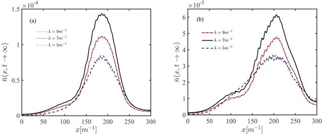
Figure 6. The position distribution for various spatial scales in electric field ( |
Previous studies also have shown that, based on the relationship between the effective action and e−e+ pair production, for a purely time-dependent electric field, the faster the field changes (corresponding to a large frequency ω), the higher the pair production rate [53, 54]. In contrast, for a purely space-dependent electric field, the faster the field changes (corresponding to a small spatial scale λ), the lower the pair production rate[53]. Now it is noted that our electric field model equation(38 ) is composed of the space and time dependence, and we find that when ωm = 0.07 or ωm = 0.1, the variation of particle number with spatial scales is non-monotonic, as shown in figure 5(b). Since there is a delicate interaction between photon energy and field focusing [36, 38, 43] there is nonlinear variation in the pair production process. This is particularly interesting if our goal is to optimize the particle number within a given range of laser parameters. It can achieve a small total energy input by the laser but the number of created particles is large.
In order to study the effect of modulated frequency and amplitude on the reduced particle number more comprehensively, we present the contour plot, as shown in figure 7. Due to limited computational resources, we select an intermediate spatial scale λ = 100 for research, meanwhile, two significant features are revealed for the reduced particle number. One is that the same particle number can be achieved through different sets of modulation parameters. The other is that the reduced particle number is very sensitive to the modulation parameters, and the particle number from region I to region IV shows an obvious nonlinear variation, i.e., it goes from small to large and then from small to large. The reasons are as follows.

Figure 7. Contour plots of the reduced particle number versus the modulated frequency and amplitude at spatial scale λ = 100. Other field parameters are E0 = 0.3Ecr, ω = 0.5, τ = 100. Note that the blank area separated by the purple solid line is beyond the modulation range of α = bωm/ω < 1. |
From figure 7, one can see that the four regions (I, II, III, IV) are divided by three typical curves, where these curves represent b = 0.06ω/ωm, b = 0.18ω/ωm and b = 0.36ω/ωm, respectively. It is noticed that there is an obvious hyperbolic relationship between modulated amplitude b and modulated frequency ωm. The maximum effective frequency ${\omega }_{{\mathrm{eff}}_{\max }}\,=\omega +b{\omega }_{m}=0.53$ corresponds to the curve b = 0.06ω/ωm, which is related to the 4-photon absorption process. The ${\omega }_{{\mathrm{eff}}_{\max }}=0.59$ corresponds to the curve b = 0.18ω/ωm, which also corresponds to 4-photon absorption. However, the ${\omega }_{{\mathrm{eff}}_{\max }}=0.68$ corresponds to the curve b = 0.36ω/ωm, which is related to the 3-photon absorption process. Therefore, the pair production processes in regions I, II, and III correspond to 4-photon absorption, while it is related to 3-photon absorption in regions IV. It is well known that the number of created particles by 3-photon absorption is much greater than that by 4-photon absorption, thus the reduced particle number is significantly enhanced in regions IV. However, for regions I, II, and III, there should not be much difference in the corresponding number of created particles, since the pair production processes all belong to 4-photon absorption, but the particle number in regions II is larger with respect to the regions I and III. This result is very interesting, though it is counterintuitive, but can be understood by the frequency spectrum structure in figure 8.
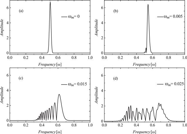
Figure 8. The frequency spectrum structure for different points A, B, C and D marked in figure 7. The corresponding modulation parameters are (a) ωm = 0, (b) ωm = 0.005, (c) ωm = 0.015 and (d) ωm = 0.025 with b = 9. Other field parameters are E0 = 0.3Ecr, ω = 0.5, τ = 100. |
To facilitate understanding of this counterintuitive result, we select the four typical points A, B, C, and D of regions I, II, III, and IV in figure 7, respectively, and give the frequency spectrum structures corresponding to these points, as shown in figure 8. It can be seen from figure 8(a), there is only one primary frequency ω = 0.5 on the frequency spectrum, while in figure 8(b), in addition to the primary frequency, two secondary frequencies appear in the spectral structure and the amplitude of the spectrum is almost the same as the case of figure 8(a), but the primary frequency is increased to ω = 0.545. Therefore, the particle number corresponding to point B is larger than that of point A, as shown in table 3. Meanwhile, from figure 8(c), it is found that there are more frequency components on the spectral structure, and the dominant frequency is increased to ω = 0.635, but the amplitude is reduced by almost half compared to the case of figure 8(b). Since in figures 8(b) and (c), the corresponding dominant frequencies are ω = 0.545 and ω = 0.635, respectively, the pair production process is related to 4-photon absorption. But the amplitude is significantly reduced in figure 8(c), which leads to a rapid decrease in the electric field strength. Therefore, the particle number corresponding to point B is significantly larger than that of point C, as shown in table 3. While in figure 8(d), we observe that there are many frequency components on the frequency spectrum, and the dominant frequency is increased to near the ω = 0.7, which means the pair production process is related to 3-photon absorption. Therefore, the particle number corresponding to point D is larger than that of A, B, and C, as shown in table 3.
Table 3. The reduced particle number for the points marked in figure 7 with different modulation regions. |
| Modulation region | Modulation parameters (ωm, b) | Reduced particle number |
|---|---|---|
| I | A(0, 9) | 6.30 × 10⁻⁴ |
| II | B(0.005, 9) | 3.42 × 10⁻² |
| III | C(0.015, 9) | 1.99 × 10⁻³ |
| IV | D(0.025, 9) | 4.54 × 10⁻² |
To study whether there are optimal modulation parameters for e−e+ pair production in a spatial inhomogeneous field with sinusoidal phase modulation, we further explore the variation of the reduced particle number in the following two cases at spatial scale λ = 100, as shown in figure 9(a). One case is that the electric field does not have any modulation, only the central frequency ω. The other case is that the electric field has both central frequency and modulation, where the central frequency is ω = 0.5, and the modulation is that the modulated frequency is fixed ωm = 0.01, but the modulated amplitude b changes. It is found that the trends of the results in the above two cases are almost identical. In the second case, we perform the Fourier transform of the time-dependent electric field and regard the frequency with the largest amplitude on the frequency spectrum as the original center frequency of the electric field without modulation, which makes the trends almost identical. Moreover, in the first case, it is found that the reduced particle number is extremely sensitive to the central frequency of the external field and presents an obvious nonlinear variation. In particular, when the central frequency is ω = 0.69, the particle number reaches the maximum value, i.e., $\bar{N}=0.1331$, and it is significantly enhanced by more than two orders of magnitude compared to the case without modulation, i.e., ω = 0.5. In the second case, we can also observe the sensitivity of the reduced particle number to the modulated amplitude and find that when modulated frequency ωm = 0.01 and modulated amplitude b = 20.7, the reduced particle number reaches the maximum value, i,e., $\bar{N}=0.1367$, which is almost the same as the maximum value in the first case.

Figure 9. (a) Reduced particle number as a function of the central frequency of the external field (black line) when b = 0 and the modulated amplitude (red line) when ωm = 0.01 is fixed at spatial scale λ = 100, respectively. Other field parameters are E0 = 0.3Ecr, ω = 0.5, τ = 100. (b) The ratio of $\bar{N}(b=0)/\bar{N}(\omega =0.5,b=0)$, $\bar{N}({\omega }_{m}=0.01)/\bar{N}(\omega =0.5,b=0)$ as a function of the central frequency (black line) and the modulated amplitude (red line), respectively. |
Figure 9(b) shows the change in the ratio of the reduced particle number in the above two cases and the particle number under the electric field without modulation. In the first case, one can see that when the central frequency of the external field is ω = 0.69, the ratio reaches the maximum value, i.e., $\bar{N}(b=0)/\bar{N}(\omega =0.5,b=0)\approx 211$, while in the second case, when modulated frequency ωm = 0.01 and modulated amplitude b = 20.7, the maximum value of the ratio is $\bar{N}({\omega }_{m}=0.01)/\bar{N}(\omega =0.5,b=0)\approx 217$. It indicates that in the two cases, the reduced particle numbers are significantly enhanced about 200 times compared to the case without modulation, i.e., ω = 0.5. Therefore, we can obtain that ω = 0.69 is the optimal value of the central frequency of the external field to get the largest reduced particle number, meanwhile, ωm = 0.01 and b = 20.7 are the optimal values of the modulated frequency and the modulated amplitude to get the largest reduced particle number.
4. Conclusion and outlook
In summary, with the DHW formalism, we have investigated the sinusoidal phase modulation effects on the momentum spectrum and the reduced particle number in inhomogeneous fields. The effect of the spatial scale of the external field on the pair production is further examined. Meanwhile, some typical interference patterns of momentum spectra are quantitatively analyzed by bridging momentum peaks and the corresponding frequency spectra. Moreover, we compared some typical numerical results obtained by the DHW formalism with those obtained by the trajectory-based semiclassical analysis method and the LDA method. It is found that they are in good agreement.
For the momentum spectrum, a significant interference effect occurs with the increase of either modulated amplitude or frequency. Moreover, the larger amplitude modulation leads to an asymmetry of the momentum spectrum, while the frequency modulation keeps a good symmetry of the momentum spectrum.
For the reduced particle number, it is significantly enhanced by the variation of modulation parameters for different spatial scales. At small spatial scales, compared with the case without modulation, the particle number is enhanced by more than one order of magnitude with modulated amplitude, while it is increased about 5 times with modulated frequency. At large spatial scales, the particle number is increased by more than one order of magnitude with modulation parameters. When modulation parameters are fixed, the reduced particle number increases rapidly with the increase of spatial scale at small spatial scales, while it tends to be a constant at large spatial scales.
Importantly, it is found that the particle number at small spatial scales is larger than that in the case of large spatial scales when modulation parameters are fixed (ωm = 0.07 and 0.1). It indicates that the total energy input by the laser is small, but the number of created particles is large. Therefore, our electric field model provides a possibility to achieve high efficiency e−e+ pair production. Moreover, it is found that for an obtained particle number, it can be achieved by different sets of modulation parameters when spatial scales are fixed. This is important since it can provide more freedom in parameter selection for pair production. Therefore, by combining the above two effects of the spatial scale in inhomogeneity of the fields and the different ways of modulation, we can effectively achieve the optimal pair production with the more flexible parameter selection.
Our study indicates that the sinusoidal phase modulation would play a crucial role in e−e+ pair production under spatially inhomogeneous electric fields, meanwhile, it also provides a possibility of broader parameter ranges for realizing the optimal pair production. While we have only considered e−e+ pair production in a single field, it is believed that the presented scheme about the phase modulation can be extended to the case of multiple fields, in which the dynamically assisted effect is included.