


1. Introduction
Heavy flavor production in high energy collision provides the crucial test of Quantum Chromodynamics, while the accuracy of the test nevertheless relies on the nonperturbative process of hadronization. The partons in the early stage after hard collisions can be measured as jets reconstructed by the final hadrons. Hence it is an interesting measurement to study the hadronization through the jet structure, for example, the hadron distributions inside jets. Such a measurement has been widely studied in various scattering processes. In heavy ion collision, this measurement puts a crucial test on various jet quenching models [1]. In hadronic scattering, this measurement helps to investigate the hadronization mechanisms. Recently, the ATLAS collaboration has reported the D*± meson production in jets from pp collision [2]. The Monte Carlo predictions in the traditional framework of fragmentation fail to describe the data for the D*± mesons carrying a small fraction of the jet momentum. Studies for the modified fragmentation functions including the high order corrections have been proposed to eliminate the discrepancy [3, 4]. They suggested enhancing the gluon fragmentation function by a factor of 2, then the calculation leads to a better agreement with the data. On the other hand, it has long been recognized that hadrons with modest momenta where the multiplicity is large receive contributions from the (re)combination mechanism. In this paper, we investigate the contribution of the combination of the charm quark with the light one nearby in phase space to produce the D* meson. The underlying events can provide the sources for the light quark to be combined.
Quark combination mechanisms and practical models have been widely studied for a very long time in various scattering processes. Among all the studies, the most relevant ones for this work are those from the viewpoint of perturbative Quantum Chromodynamics (pQCD) [5, 6]. Some years ago, we proposed the pQCD factorized formulation for a heavy quark produced from the hard scattering combined with a light one from the background environment to produce the heavy meson [7]. The obtained cross section of the inclusive scattering process A + B → MQ + X (where MQ denotes the produced heavy meson) is the convolution of the hard sub-cross section of the heavy quark production $A+B\to Q\bar{Q}+X$, the combination matrix element and the parameter (matrix element) corresponding to the parton distributions in the background. The combination matrix element and the parton distribution of the background are expectation values of field operators on certain states, so they are model-independent and could be calculated by lattice QCD. The combination matrix element describes the possibility of a heavy quark and a light one of specified momenta to form a heavy hadron. Within the same factorization scheme, it can appear in other more ‘simple and clean' processes, so it can be extracted from the experiments. The process-relevant factor is the spectrum of the heavy quark, which can be calculated by pQCD. Now, full NLO corrections are available [8, 9]. We suspected that this mechanism could be globally studied in various scattering processes, to quantify the universal combination matrix elements. Such a study, and vice versa, could play a role as a scaling probe on the background parton distribution, e.g., that of the quark gluon plasma in the relativistic heavy ion collisions, especially after the universal combination matrix elements are fixed [7]. Now the available data for charm meson distributions in a jet from pp scattering [2] provide a good opportunity to study the combination mechanism as well as to probe the light quark distributions from the underlying events.
The outline of this paper is as follows: In section 2 we introduce the factorization framework for the case perturbatively-produced charm quark combing with the light one from the underlying events and derive the cross section formula. In section 3 we calculate the D*± distribution in jet R(pT, z). The combination matrix element and the light quark distribution are not yet available from experimentation currently. We study the sensitivity of the R(pT, z) to them. With some physical conjectures, we calculate the D*± production in jet via combination in pp collisions at the LHC. It is summed with the fragmentation contribution, and the total result is comparable with the experimental data [2]. In section 4 , we discuss some properties of the combination mechanism studied in this paper.
2. Cross section for combination of heavy quark with light one
In this section, we take the hadronic collision $A\,+B\to {\bar{D}}^{* }+X$ as an example (see figure 1). Here ${\bar{D}}^{* }$ refers to any anti-charm meson. The formula is the same when applied to the charm quark case. However, in experiments, one studies prompt D* rather than prompt D because the former does not need to consider the decay contribution. We only consider the contribution of $\bar{c}+q$ to ${\bar{D}}^{* }$, other possible combination processes such as $\bar{c}+g$ to ${\bar{D}}^{* }$ are assumed negligible. The X includes the associated produced c quark and the other particles from the incident particles A, B interaction. We obtain the invariant inclusive differential production cross section $2E\tfrac{{\rm{d}}{\sigma }_{C}^{{AB}}}{{{\rm{d}}}^{3}{\boldsymbol{K}}}$ of ${\bar{D}}^{* }$. The subscribe C of σ denotes the combination process. (E, K) is the 4-momentum of ${\bar{D}}^{* }$. The production of charm mesons can be treated in the same way as the anti-charm mesons. To describe the light quark to be combined, we should find ways to represent the ‘external particle source'. We introduce an external vector field Vμ which, together with light quark field operators, appears in the matrix element corresponding to the light quark distribution. The external field is proportional to nμ = (n+, n−, n⊥) = (0, 1, 0⊥), which is consistent with the collinear factorization framework. Here we employ the light-cone variables, with ${n}^{+}=\tfrac{1}{\sqrt{2}}({n}^{0}+{n}_{z})$ and ${n}^{-}=\tfrac{1}{\sqrt{2}}({n}^{0}-{n}_{z})$.

Figure 1. ${\bar{D}}^{* }$ production at the proton-proton collider. Here the charm quark can be produced via various partonic hard processes, for details see section |
From the above discussions, the interaction Hamiltonian for quark and gluon fields is extended as [10]:
$\begin{eqnarray}{H}_{I}=\bar{{\rm{\Psi }}}(\rlap{/}{A}+\rlap{/}{V}){\rm{\Psi }}.\end{eqnarray}$
Here A is the normal gluon field and V is the external field. The $\Psi$ is for the fermion (quark) field. The strong coupling constant gs is absorbed into the gauge fields. In this paper, wherever we write the gauge field obviously, we always adopt this convention. If we assume that the distribution functions of the intrinsic heavy flavours in the initial state AB are vanishing, the lowest order contribution for the combination process comes from $O({g}_{s}^{3})$ in the perturbative expansion of the S-matrix: $\begin{eqnarray}\begin{array}{rcl}{S}^{(3)} & = & \displaystyle \frac{{\left(-{\rm{i}}\right)}^{3}}{3!}\displaystyle \frac{1}{3}\displaystyle \int {{\rm{d}}}^{4}{x}_{1}{{\rm{d}}}^{4}{x}_{2}{{\rm{d}}}^{4}{x}_{3}{\bf{T}}\bar{{\rm{\Psi }}}({x}_{1})\rlap{/}{A}({x}_{1}){\rm{\Psi }}({x}_{1})\\ & & \times \bar{{\rm{\Psi }}}({x}_{2})\rlap{/}{A}({x}_{2}){\rm{\Psi }}({x}_{2})\bar{{\rm{\Psi }}}({x}_{3})\rlap{/}{V}({x}_{3}){\rm{\Psi }}({x}_{3}),\end{array}\end{eqnarray}$
where summation on colour and flavour indices, as well as the indices in spinor space, are indicated. T indicates time-ordered products.Now we take the annihilation partonic process $q\bar{q}\to c\bar{c}$ as an example of the partonic processes to illustrate the derivation, while the total result can be obtained by summing all kinds of partonic processes. Let the corresponding terms of the Wick expansion act on the initial state $\left|{AB}\right\rangle $ and final state $\left|{\bar{D}}^{* }X\right\rangle $, employing the space-time translation invariance, we can isolate the δ function corresponding to the total energy-momentum conservation and get the T-matrix element. The cross section then is
$\begin{eqnarray}\begin{array}{rcl}\sigma & = & \displaystyle \frac{{\left(4\pi {\alpha }_{s}\right)}^{2}}{4F}\displaystyle \sum _{{\bar{D}}^{* }X}\displaystyle \int {{\rm{d}}}^{4}{x}_{1}{{\rm{d}}}^{4}{x}_{2}{{\rm{d}}}^{4}{x}_{3}{{\rm{d}}}^{4}{x}_{4}{{\rm{d}}}^{4}{x}_{5}\\ & & \times \displaystyle \int \displaystyle \frac{{{\rm{d}}}^{4}q}{{\left(2\pi \right)}^{4}}\displaystyle \frac{{{\rm{d}}}^{4}q^{\prime} }{{\left(2\pi \right)}^{4}}\displaystyle \frac{1}{{q}^{2}q{{\prime} }^{2}}{{\rm{e}}}^{-{\rm{i}}q({x}_{1}-{x}_{2})}{{\rm{e}}}^{{\rm{i}}q^{\prime} ({x}_{4}-{x}_{5})}\\ & & \times \left\langle {AB}| \bar{\psi }({x}_{4}){T}^{{c}_{4}}{\gamma }^{{\mu }_{4}}\psi ({x}_{4})\bar{\psi }({x}_{3})\rlap{/}{V}\right.\\ & & \left.\times ({x}_{3})\psi ({x}_{3})\bar{{\rm{\Psi }}}({x}_{5}){T}^{{c}_{4}}{\gamma }_{{\mu }_{4}}{\rm{\Psi }}({x}_{5})| {\bar{D}}^{* }X\right\rangle \\ & & \times \left\langle {\bar{D}}^{* }X| \bar{{\rm{\Psi }}}({x}_{2}){T}^{{c}_{1}}{\gamma }_{{\mu }_{1}}{\rm{\Psi }}({x}_{2})\bar{\psi }(0)\rlap{/}{V}\right.\\ & & \left.\times (0)\psi (0)\bar{\psi }({x}_{1}){T}^{{c}_{1}}{\gamma }^{{\mu }_{1}}\psi ({x}_{1})| {AB}\right\rangle .\end{array}\end{eqnarray}$
In the above equation, Tc is one half of the Gell-Mann Matrix, 4F represents the incident flux factor and discrete quantum number average. Summation on repeated indices is indicated. The capital $\Psi$ is for the heavy quark field and the lower case ψ for light quark fields.In the following the cross section is simplified in the framework of collinear factorization:
$\begin{eqnarray}\sigma =\displaystyle \frac{{\left(4\pi {\alpha }_{s}\right)}^{2}C}{4F}\int \displaystyle \frac{{{\rm{d}}}^{4}q}{{\left(2\pi \right)}^{4}}{W}^{\mu \nu }\displaystyle \frac{1}{{q}^{4}}{D}_{\mu \nu },\end{eqnarray}$
with $\begin{eqnarray}\begin{array}{l}{W}^{\mu \nu }=\displaystyle \int {{\rm{d}}}^{4}{x}_{4}{{\rm{e}}}^{-{\rm{i}}{{qx}}_{4}}\left\langle A| {\bar{\psi }}^{{\alpha }_{4}}({x}_{4}){\psi }^{{\beta }_{1}}(0)| A\right\rangle \\ \quad \times \left\langle B| {\psi }^{{\beta }_{4}}({x}_{4}){\bar{\psi }}^{{\alpha }_{1}}(0)| B\right\rangle \\ \quad \times {\gamma }_{{\alpha }_{4}{\beta }_{4}}^{\mu }{\gamma }_{{\alpha }_{1}{\beta }_{1}}^{\nu }+(A\leftrightarrow B).\end{array}\end{eqnarray}$
This is the same Wμν for the Drell-Yan process, which gives the distribution of initial partons. We have employed the translation invariance and integrated on x1, which gives $q=q^{\prime} $.On the other hand,4 ), C is the colour factor of the partonic diagram except for the external leg combined into ${\bar{D}}^{* }$. The colour part will be clarified following.
$\begin{eqnarray}\begin{array}{rcl}{D}_{\mu \nu } & = & \displaystyle \int \displaystyle \frac{{{\rm{d}}}^{3}K}{{\left(2\pi \right)}^{3}2E}\displaystyle \frac{{{\rm{d}}}^{3}k^{\prime} }{{\left(2\pi \right)}^{3}2E^{\prime} }\displaystyle \int {{\rm{d}}}^{4}{x}_{2}{{\rm{d}}}^{4}{x}_{3}{{\rm{d}}}^{4}{x}_{5}{{\rm{e}}}^{-{\rm{i}}{k}_{\bar{c}}{x}_{2}}{{\rm{e}}}^{{\rm{i}}{k}_{\bar{c}}{x}_{5}}\\ & & \times {\left({\gamma }_{\mu }(\rlap{/}{k}^{\prime} +m){\gamma }_{\nu }\right)}_{{\alpha }_{5}{\beta }_{2}}\left\langle 0| {\left(\bar{\psi }({x}_{3})\rlap{/}{V}({x}_{3})\right)}_{{\beta }_{3}}^{{j}_{3}}| {X}_{h}\right\rangle \\ & & \times \displaystyle \sum _{{X}_{h}}\left\langle {X}_{h}| {\left(\rlap{/}{V}(0)\psi (0)\right)}_{{\alpha }_{0}}^{{j}_{0}}| 0 \right\rangle \times \left\langle 0| {\psi }_{{\beta }_{3}}^{{j}_{3}}({x}_{3}){\bar{{\rm{\Psi }}}}_{{\alpha }_{5}}^{j}({x}_{5})| {\bar{D}}^{* }\right\rangle \\ & & \times \,\left\langle {\bar{D}}^{* }| {{\rm{\Psi }}}_{{\beta }_{2}}^{j}({x}_{2}){\bar{\psi }}_{{\alpha }_{0}}^{{j}_{0}}(0)| 0\right\rangle .\end{array}\end{eqnarray}$
To get the above expression, we have written the total final state produced in the AB collision as $\left|{\bar{D}}^{* }X\right\rangle =\left|{\bar{D}}^{* }\tilde{X}{{cX}}_{h}\right\rangle $, where the $\tilde{X}$ represents all the particles except the $c\bar{c}$ produced by the hard interaction and Xh for the assembly of particles produced by all the interactions except the above hard one. We have the corresponding field acting on the c quark final state with momentum $k^{\prime} $, ${k}_{\bar{c}}=q-k^{\prime} $. The summation on $\tilde{X}$ has been eliminated by the completeness condition. In equation (The Wμν can be conventionally written as
$\begin{eqnarray}\begin{array}{l}\displaystyle \int \displaystyle \frac{{{\rm{d}}}^{4}q}{{\left(2\pi \right)}^{4}}{W}^{\mu \nu }=\displaystyle \int {\rm{d}}{r}_{1}{\rm{d}}{r}_{2}\displaystyle \int \displaystyle \frac{{\rm{d}}{\lambda }_{1}}{2\pi }\displaystyle \frac{{\rm{d}}{\lambda }_{2}}{2\pi }{{\rm{e}}}^{-{\rm{i}}{r}_{1}{\lambda }_{1}}{{\rm{e}}}^{-{\rm{i}}{r}_{2}{\lambda }_{2}}\\ \quad \times \left\langle A\right|\bar{\psi }(y)\displaystyle \frac{{\gamma }^{+}}{2{P}_{1}^{+}}\psi (0)\left|A\right\rangle \\ \quad \times \left\langle B\right|{\rm{tr}}\left(\displaystyle \frac{{\gamma }^{-}}{2{P}_{2}^{-}}\psi (y)\bar{\psi }(0)\right)\left|B\right\rangle \\ \quad \times {\rm{tr}}\left(\displaystyle \frac{{\rlap{/}{P}}_{1}}{2}{\gamma }^{\mu }\displaystyle \frac{{\rlap{/}{P}}_{2}}{2}{\gamma }^{\nu }\right),\end{array}\end{eqnarray}$
which is the intended factorized form. Some of the above variables are: ${\lambda }_{1}={P}_{1}^{+}{y}_{-},{\lambda }_{2}={P}_{2}^{-}{y}_{+}$, y = (y+, y−, 0⊥), Q2 ≡ q2 = r1r2s, s is the center of mass frame (c.m.s) energy for the AB system whose partons collide and produce the heavy quark pair.The factorization for Dμν is more complicated. It can be written as:
$\begin{eqnarray}\begin{array}{l}\displaystyle \int \displaystyle \frac{{{\rm{d}}}^{3}K}{{\left(2\pi \right)}^{3}2E}{\rm{d}}\xi {K}^{+}{\rm{d}}{\xi }_{l}{K}^{+}(2\pi )\delta (k{{\prime} }^{2}-{m}^{2})\\ \quad \times {\left(2\pi \right)}^{4}{\delta }^{4}({k}_{l}+{k}_{\bar{c}}-K)\\ \quad \times {\rm{tr}}{\left({\gamma }_{\mu }(\rlap{/}{k}^{\prime} +m){\gamma }_{\nu }\left.\displaystyle \frac{\rlap{/}{K}}{2}\right)\right|}_{k^{\prime} =q-\xi {K}^{+}}\\ \quad \times \displaystyle \int {{\rm{d}}}^{4}{x}_{3}{{\rm{e}}}^{-{\rm{i}}{k}_{l}{x}_{3}}{| }_{{k}_{l}^{+}={\xi }_{l}{K}^{+}}\left\langle 0| {\left({V}_{n}({x}_{3})\bar{\psi }({x}_{3})\right)}_{{j}_{0}}| {X}_{h}\right\rangle \\ \quad \times \displaystyle \sum _{{X}_{h}}\left\langle {X}_{h}\right|\displaystyle \frac{{\gamma }^{+}}{2{K}^{+}}{\left(\psi (0){V}_{n}(0)\right)}_{{j}_{0}}\left|0\right\rangle \\ \quad \times \displaystyle \frac{1}{9}\displaystyle \int \displaystyle \frac{{{\rm{d}}}^{4}{k}_{\bar{c}}}{{\left(2\pi \right)}^{4}}\displaystyle \frac{{{\rm{d}}}^{4}{k}_{l}}{{\left(2\pi \right)}^{4}}\delta \left(\xi -\displaystyle \frac{{k}_{\bar{c}}^{+}}{{K}^{+}}\right)\delta \left({\xi }_{l}-\displaystyle \frac{{k}_{l}^{+}}{{K}^{+}}\right)\\ \quad \times \displaystyle \int {{\rm{d}}}^{4}{x}_{2}{{\rm{d}}}^{4}{x}_{5}{{\rm{e}}}^{-{\rm{i}}{k}_{\bar{c}}{x}_{2}}{{\rm{e}}}^{{\rm{i}}{k}_{l}{x}_{5}}\\ \quad \times \left\langle 0\right|{\rm{tr}}(\displaystyle \frac{{\gamma }^{+}}{2{K}^{+}}{\psi }^{{j}_{0}}({x}_{5}){\bar{{\rm{\Psi }}}}^{j}(0))\left|{\bar{D}}^{* }\right\rangle \\ \quad \times \left\langle {\bar{D}}^{* }\right|{\rm{tr}}\left(\displaystyle \frac{{\gamma }^{+}}{2{K}^{+}}{{\rm{\Psi }}}^{j}({x}_{2}){\bar{\psi }}^{{j}_{0}}(0)\right)\left|0\right\rangle .\end{array}\end{eqnarray}$
In the above equation, the colour indices in the partonic final states and the distribution functions are summed. So the colour indices in the combination matrix elements should be averaged $\left(\tfrac{1}{9}\right)$, which is similar to the case in the fragmentation function. We do not separate the colour-singlet or the colour-octet contribution in the matrix elements but sum them together. The reason is that the partonic cross section is the same for the colour indices j belonging to $\underline{1}$ or $\underline{8}$ states (since the other parton comes from an un-correlated source), and that for the parton distribution, it should be the same whether j0 belongs to $\underline{1}$ or $\underline{8}$ states. We have taken the external field proportional to nμ, which selects only the ‘+' component since $\rlap{/}{n}{\rlap{/}{K}}^{-}\rlap{/}{n}=\rlap{/}{n}{\rlap{/}{{\boldsymbol{K}}}}_{\perp }\rlap{/}{n}=0$. In the part corresponding to the partonic sub-process, for the sake of factorization, we have done the collinear expansion for the momentum of the $\bar{c}$ along the ‘+' component of the momentum of ${\bar{D}}^{* }$. Here one notices that the coordinate system is different from that for initial states Wμν. The z − axis direction is along the momentum of the anti-charm meson.In equation (8 ), we write the combination matrix element (Row 4, 5) formally to be analogous to that in other processes (see following discussions). ξ and ξl seem not restricted to be ξ + ξl = 1. However, the δ functions in the first row set the restriction. At the same time, the integral in the combination matrix elements ∫d4kl acts on the matrix element corresponding to the quark distribution represented by the external field (Row 3) as well as the δ function in the first row. These show that we have not finished the factorization. To get the factorized form, we notice
$\begin{eqnarray}\begin{array}{l}\displaystyle \int \displaystyle \frac{{{\rm{d}}}^{3}K}{2E}{\delta }^{4}({k}_{l}+{k}_{\bar{c}}-K)\\ \quad =\displaystyle \int \displaystyle \frac{{\rm{d}}{K}^{-}{{\rm{d}}}^{2}{K}_{\perp }}{2{K}^{-}}{\delta }^{+}({k}_{l}^{+}+{k}_{\bar{c}}^{+}-{K}^{+}){\delta }^{-}{\delta }_{\perp }^{2}\\ \quad =\displaystyle \int \displaystyle \frac{{{\rm{d}}}^{3}K}{2E}2E{\delta }^{3}({{\boldsymbol{k}}}_{\bar{c}}+{{\boldsymbol{k}}}_{l}-{\boldsymbol{K}})\\ \quad \times \displaystyle \frac{1}{2{K}^{-}}{\delta }^{+}({k}_{l}^{+}+{k}_{\bar{c}}^{+}-{K}^{+}).\end{array}\end{eqnarray}$
Let the 3-dimension δ function absorbed into the combination matrix element, we get the ‘restricted' matrix element or the dimensionless combination function: $\begin{eqnarray}\begin{array}{l}\tilde{F}(\xi ,{\xi }_{l})=\displaystyle \frac{1}{9}\displaystyle \int \displaystyle \frac{{{\rm{d}}}^{4}{k}_{\bar{c}}}{{\left(2\pi \right)}^{4}}\delta \left(\xi -\displaystyle \frac{{k}_{\bar{c}}^{+}}{{K}^{+}}\right)\\ \quad \times \displaystyle \frac{{{\rm{d}}}^{4}{k}_{l}}{{\left(2\pi \right)}^{4}}\delta \left({\xi }_{l}-\displaystyle \frac{{k}_{l}^{+}}{{K}^{+}}\right)\\ \quad \times \displaystyle \int {{\rm{d}}}^{4}{x}_{2}{{\rm{d}}}^{4}{x}_{5}{{\rm{e}}}^{-{\rm{i}}{k}_{\bar{c}}{x}_{2}}{{\rm{e}}}^{{\rm{i}}{k}_{l}{x}_{5}}\\ \quad \times \left\langle 0\left|{\rm{tr}}\left(\displaystyle \frac{{\gamma }^{+}}{2{K}^{+}}{\psi }^{{j}_{0}}({x}_{5}){\bar{{\rm{\Psi }}}}^{j}(0)\right)\right|{\bar{D}}^{* }\right\rangle \\ \quad \times \left\langle {\bar{D}}^{* }\right|{\rm{tr}}\left(\displaystyle \frac{{\gamma }^{+}}{2{K}^{+}}{{\rm{\Psi }}}^{j}({x}_{2}){\bar{\psi }}^{{j}_{0}}(0)\right)\left|0\right\rangle \\ \quad \times 2E{\delta }^{3}\left({{\boldsymbol{k}}}_{\bar{c}}+{{\boldsymbol{k}}}_{l}-{\boldsymbol{K}}\right).\end{array}\end{eqnarray}$
The integral of ξl in the first row of equation (8 ) has given ξ + ξl = 1. $\int {\rm{d}}\xi \delta (k{{\prime} }^{2}-{m}^{2})$ gives the important result: $\xi =\tfrac{{Q}^{2}}{2K\cdot q}$,4(4This relation is exact for Q and K to be infinite while z is fixed. It is a good approximation when the anti-quark to be combined into the heavy meson is on a mass shell in the partonic processes. In this case, the four-momentum of the anti-quark is $(\xi {K}^{+},\tfrac{{m}^{2}}{2\xi {K}^{+}},{0}_{\perp })$. In the heavy meson rest frame, it is easy to get $\xi =\tfrac{\sqrt{{m}^{2}+{\left({mv}\right)}^{2}}+{mv}}{M}\simeq \tfrac{m}{M}$. Go back to the initial parton c.m.s, using this approximation for the on-shell condition ${\left(q-k\right)}^{2}\,=\,{m}^{2}$, we can get the relation. So, it is not just an approximation by taking M = mc = 0 in K · q.) which is analogous to the Bjorken scaling variable. This means that for certain partonic c.m.s energy Q, the heavy meson with momentum K just comes from the heavy quark with the momentum fraction ξ combined with the light quark with the momentum kl = (1 − ξ)K, and hence only probes this light quark by the combination mechanism. Such a conclusion does not depend on the special forms of the derivation in this paper. In fact, the relation $\xi =\tfrac{{Q}^{2}}{2K\cdot q}$ is set by the on-shell condition of the heavy quark associatively produced with the one to be combined into the final state heavy hadron. Just like the DIS process, this is a physical condition that should be respected by any special forms of derivation.
The cross section now can be written as
$\begin{eqnarray}\begin{array}{l}2E\displaystyle \frac{{\rm{d}}{\sigma }_{C}}{{{\rm{d}}}^{3}K}=\displaystyle \frac{1}{4F}\displaystyle \sum _{{ab}}\displaystyle \int {\rm{d}}{r}_{1}{\rm{d}}{r}_{2}2{f}_{A}^{a}({r}_{1})2{f}_{B}^{b}({r}_{2})\\ \quad \times | {\tilde{{ \mathcal M }}}_{{ab}}{| }^{2}\displaystyle \frac{1}{\xi }\displaystyle \frac{{\left(2\pi \right)}^{2}}{{\left(2M\right)}^{2}}2P({\xi }_{l})\tilde{F}(\xi ,{\xi }_{l}){| }_{\xi +{\xi }_{l}=1}.\end{array}\end{eqnarray}$
Here ${f}_{A}^{a}({r}_{1})$ and ${f}_{B}^{b}({r}_{2})$ are parton distributions with momentum factions r1, r2. a and b run over all kinds of partons including $q\bar{q}$ and gg cases at lowest order. M is the mass of the heavy meson. $| \tilde{{ \mathcal M }}{| }^{2}$ refers to the invariant amplitude square including all the coupling constant and colour factors for the partonic process ${ab}\to \bar{c}+x$ (where the momenta of external legs are modified and x is to be considered as one particle). For example, for $q\bar{q}\to \bar{c}+x$, to the lowest order, $| \tilde{{ \mathcal M }}{| }^{2}$ is $\begin{eqnarray}{\left(4\pi {\alpha }_{s}\right)}^{2}C^{\prime} {\rm{tr}}\left(\displaystyle \frac{{\rlap{/}{P}}_{1}}{2}{\gamma }^{\mu }\displaystyle \frac{{\rlap{/}{P}}_{2}}{2}{\gamma }^{\nu }\right)\displaystyle \frac{1}{{q}^{4}}{\rm{tr}}\left({\gamma }_{\mu }(\rlap{/}{k}^{\prime} +m){\gamma }_{\nu }\displaystyle \frac{\rlap{/}{K}}{2}\right).\end{eqnarray}$
$C^{\prime} $ is the colour factor. Though the quark mass term is vanishing, we keep it to show the origin of the formula. The gluon–gluon fusion process can be obtained in a similar way.P(ξl) can be understood as the distribution function of the parton (probed by the heavy quark). P(ξl) is also dimensionless:
$\begin{eqnarray}\begin{array}{l}\displaystyle \frac{1}{2}\displaystyle \int {{\rm{d}}}^{4}{x}_{3}{{\rm{e}}}^{-{\rm{i}}{k}_{l}{x}_{3}}{| }_{{k}_{l}^{+}={\xi }_{l}{K}^{+}}\displaystyle \sum _{{X}_{h}}\left\langle {X}_{h}| {\rm{tr}}(\psi (0){V}_{n}(0)| 0\right\rangle \\ \quad \times \left\langle 0\right|{V}_{n}({x}_{3})\bar{\psi }({x}_{3})\displaystyle \frac{{\gamma }^{+}}{2{K}^{+}})\left|{X}_{h}\right\rangle .\end{array}\end{eqnarray}$
This can be understood as the expectation value on the state representing an assembly of particles produced in the AB collision denoted by $\left|{X}_{h}\right\rangle $, e.g., those from the underlying events.We get the cross section of the production of ${\bar{D}}^{* }$ in the combination process:
$\begin{eqnarray}\begin{array}{l}2E\displaystyle \frac{{\rm{d}}{\sigma }_{C}}{{{\rm{d}}}^{3}K}=\displaystyle \sum _{{ab}}\displaystyle \int {\rm{d}}{r}_{1}{\rm{d}}{r}_{2}{f}_{1}^{a}({r}_{1}){f}_{2}^{b}({r}_{2})\\ \quad \times \displaystyle \frac{{\rm{d}}{\hat{\sigma }}_{{ab}}}{{\rm{d}}{ \mathcal I }}\displaystyle \frac{1}{{\xi }^{2}}\displaystyle \frac{{\left(2\pi \right)}^{2}}{{\left(2M\right)}^{2}}P({\xi }_{l})\tilde{F}(\xi ,{\xi }_{l}){| }_{\xi +{\xi }_{l}=1}.\end{array}\end{eqnarray}$
In the above equation, ${\rm{d}}{ \mathcal I }$ is the dimensionless invariant phase space for the ‘2-body' partonic final state $\bar{c}+x$ where x is treated as one particle. This formula is also correct for higher order partonic cross sections.As shown in the above equation, the cross section of the ${\bar{D}}^{* }$ is dependent on both the combination matrix element and the distribution of the light quark, which are not calculable by pQCD. We should find ways to extract from more ‘simple' experiments or conjecture some models. The light quark distribution P(ξl) is easier to be modeled, inspired by the available data and theory for certain cases. There is a special property that P(ξl) is dependent on the specific ‘background', i.e., vacuum, comoving partons in a jet, underlying events, quark–gluon plasma, or even curved space-time, etc. So, its normalization is not definite, nor can some sum rules exist as those of the parton distribution for nucleons. This can be easily recognized by noticing that the matrix element includes the ‘classical' external field, which is ‘macroscopic', rather than statistical. Such a case generally can not be described by a pure state. The classical external field can take any value. The corresponding physics is that the light quark to be combined with the heavy one comes from a source that is dependent on the evolution in details specified by the concrete collision process.
On the other hand, the combination function $\tilde{F}(\xi ,{\xi }_{l})$ is not intuitive. So the model it is difficult to construct the model. Furthermore, the normalization is also not definite. From the definition above, we can only mention that its normalization is smaller than 1 once the vacuum and particle states are normalized to be 1. It is different from the naive parton distribution function because there the process has been fixed to the case that the hard projectile must hit on one parton (e.g. the virtual photon hitting the parton in the DIS process). But here we conjecture this combination process to be added to the fragmentation process as a high twist correction (see below equation (20 )). However, if the cross section of a more simple process can be factorized and includes this parameter, it can be extracted from data. The following is an example. Let's see the factorization and the complexity.
It has been pointed out that, in hadronic interaction, the asymmetry of a D meson in the forward direction can be explained by the combination of the initial parton with the charm quark produced in the hard interaction. Such a leading particle effect has been studied in [11–14], both in the approximation mc → ∞ . In such an approximation, the light quark has vanishing momentum, hence, qualitatively, the momentum of the D meson is approximately that of the charm quark, so that not possible to probe the momentum of the light quark, but leaving a non-relativistic combination matrix. On the other hand, in [15], the authors also tried to give the combination matrix elements in the framework of collinear factorization, which is the same framework used in this paper. The combination matrix elements there depend on three variables z1, z2, z3, which seem not to correspond to the momentum fraction of the valence partons. However, starting from equation (4) in [14], by taking into account the space-time transition invariance, we get the combination matrix elements with two variables corresponding to the momentum fraction of the charm and the light quarks, which is like those in the above section:
$\begin{eqnarray}\begin{array}{l}\displaystyle \int \displaystyle \frac{{{\rm{d}}}^{4}{k}_{c}}{{\left(2\pi \right)}^{4}}\displaystyle \frac{{{\rm{d}}}^{4}{k}_{l}}{{\left(2\pi \right)}^{4}}\delta \left(\xi -\displaystyle \frac{{k}_{c}^{+}}{{K}^{+}}\right)\delta \left({\xi }_{l}-\displaystyle \frac{{k}_{l}^{+}}{{K}^{+}}\right)\\ \quad \times \displaystyle \int {{\rm{d}}}^{4}{x}_{1}{{\rm{d}}}^{4}{x}_{2}{{\rm{e}}}^{{\rm{i}}{k}_{c}{x}_{1}}{{\rm{e}}}^{-{\rm{i}}{k}_{l}{x}_{2}}\\ \quad \times \left\langle 0\right|{\bar{q}}_{k}(0)\displaystyle \frac{{\gamma }^{+}}{2{K}^{+}}{Q}_{l}({x}_{1}))\left|{H}_{Q}\right\rangle \\ \quad \times \left\langle {H}_{Q}\right|{\bar{Q}}_{i}(0)\displaystyle \frac{{\gamma }^{+}}{2{K}^{+}}{q}_{j}({x}_{2}))\left|0\right\rangle ,\end{array}\end{eqnarray}$
and $\begin{eqnarray}\begin{array}{l}\displaystyle \int \displaystyle \frac{{{\rm{d}}}^{4}{k}_{c}}{{\left(2\pi \right)}^{4}}\displaystyle \frac{{{\rm{d}}}^{4}{k}_{l}}{{\left(2\pi \right)}^{4}}\delta \left(\xi -\displaystyle \frac{{k}_{c}^{+}}{{K}^{+}}\right)\delta \left({\xi }_{l}-\displaystyle \frac{{k}_{l}^{+}}{{K}^{+}}\right)\\ \quad \times \displaystyle \int {{\rm{d}}}^{4}{x}_{1}{{\rm{d}}}^{4}{x}_{2}{{\rm{e}}}^{{\rm{i}}{k}_{c}{x}_{1}}{{\rm{e}}}^{-{\rm{i}}{k}_{l}{x}_{2}}\\ \quad \times \left\langle 0\right|{\bar{q}}_{k}(0)\displaystyle \frac{{\gamma }^{5}{\gamma }^{+}}{2{K}^{+}}{Q}_{l}({x}_{1}))\left|{H}_{Q}\right\rangle \\ \quad \times \left\langle {H}_{Q}\right|{\bar{Q}}_{i}(0)\displaystyle \frac{{\gamma }^{5}{\gamma }^{+}}{2{K}^{+}}{q}_{j}({x}_{2}))\left|0\right\rangle .\end{array}\end{eqnarray}$
These two parts of the combination matrix element, i.e., the double-vector part and the double-pseudo-vector part, should be separated since the partonic cross sections corresponding to these two parts could be different. In the case that the quark and the anti-quark are from different sources respectively, these two parts can be put together and only the vector part needs consideration.The complexity lies in that, equations (15 ), (16 ) are different from that in equation (10 ) by $2E{\delta }^{3}({{\boldsymbol{k}}}_{\bar{c}}+{{\boldsymbol{k}}}_{l}-{\boldsymbol{K}})$, without the restriction ξ + ξl = 1. The reason is that in the process in [14], the light quark and the heavy quark can undergo hard interactions and in principle are not restricted to the on mass shell. We can also understand this in a different way. Equations (15 ) and (16 ) look like the combined distribution of two valence quarks in the heavy meson. In fact, rewriting the $\left\langle 0\right|{\left(\cdot \cdot \cdot \right)}_{1}\left|{H}_{Q}\right\rangle \left\langle {H}_{Q}\right|{\left(\cdot \cdot \cdot \right)}_{2}\left|0\right\rangle $ to the form $\left\langle {H}_{Q}\right|{\left(\cdot \cdot \cdot \right)}_{2}\left|0\right\rangle \left\langle 0\right|{\left(\cdot \cdot \cdot \right)}_{1}\left|{H}_{Q}\right\rangle $, integrating the δ functions and the exponential functions, taking $\left|0\right\rangle \left\langle 0\right|=1$ in the vacuum saturation approximation, we will get the form of the product of two parton distribution functions, each similar to that defined by Collins and Soper [15]. Then in a parton model at high energy, we can not require the sum of two parton momentum fractions to equal one. Hence to get the inputs needed, we should find ways to relate the ‘restricted' one above with this ‘unrestricted'.
If the unrestricted matrix elements have been extracted from experiments, to get the restricted combination function, we start by denoting the Combination Matrix Element in equations (15 , 16 ) as CME:
$\begin{eqnarray}\begin{array}{rcl}{CME} & = & \displaystyle \int \displaystyle \frac{{{\rm{d}}}^{3}K^{\prime} }{2E^{\prime} }2E^{\prime} {\delta }^{3}({{\boldsymbol{k}}}_{c}^{{\prime} }+{{\boldsymbol{k}}}_{l}^{{\prime} }-{\boldsymbol{K}}^{\prime} )\\ & & \times \displaystyle \frac{{{\rm{d}}}^{3}{k}_{c}^{{\prime} }}{2{E}_{c}^{{\prime} }}2{E}_{c}^{{\prime} }{\delta }^{3}({{\boldsymbol{k}}}_{c}^{{\prime} }-{{\boldsymbol{k}}}_{c})\\ & & \times \displaystyle \frac{{{\rm{d}}}^{3}{k}_{l}^{{\prime} }}{2{E}_{l}^{{\prime} }}2{E}_{l}^{{\prime} }{\delta }^{3}({{\boldsymbol{k}}}_{l}^{{\prime} }-{{\boldsymbol{k}}}_{l}){CME}\\ & = & \displaystyle \int \displaystyle \frac{{{\rm{d}}}^{3}K^{\prime} }{2E^{\prime} }\tilde{F}(\xi ,{\xi }_{l};\xi +{\xi }_{l}).\end{array}\end{eqnarray}$
In principle, we should solve the integral equation and use the value of $\tilde{F}$ on ξ + ξl = 1 (${\boldsymbol{K}}^{\prime} ={\boldsymbol{K}}$) as our inputs. On the other hand, if the real world is more simple as most models assume, $\tilde{F}(\xi ,{\xi }_{l};\xi +{\xi }_{l})$ peaks around ξ + ξl = 1, i.e., two valence quarks on mass shell with kc + kl ≃ K, we can approximately fit CME as, $\begin{eqnarray}\begin{array}{l}{CME}=\displaystyle \int \displaystyle \frac{{{\rm{d}}}^{3}K^{\prime} }{2E^{\prime} }2E^{\prime} {\prod }_{i}\displaystyle \frac{{\epsilon }_{i}}{\pi ({\epsilon }_{i}^{2}+{\left({\boldsymbol{K}}-{\boldsymbol{K}}^{\prime} \right)}_{i}^{2})}{M}^{2}f(\xi ,{\xi }_{l})\\ \quad \mathop{=}\limits_{({\epsilon }_{i}\to 0)}\displaystyle \int \displaystyle \frac{{{\rm{d}}}^{3}K^{\prime} }{2E^{\prime} }2E^{\prime} {\delta }^{3}({\boldsymbol{K}}-{\boldsymbol{K}}^{\prime} ){M}^{2}f(\xi ,{\xi }_{l}).\end{array}\end{eqnarray}$
So in the extreme/ideal condition, we can just have $\tilde{F}{\left(\xi ,{\xi }_{l}\right)}_{\xi +{\xi }_{l}=1}\propto \tfrac{{CME}}{{M}^{2}}$. That is because the distribution of $\tilde{F}$ is a narrow peak, we use the average value of it in a reasonably small integral region of $\tfrac{{{\rm{d}}}^{3}K^{\prime} }{2E^{\prime} }$.Equations (15 ) and (16 ) will be applied in other processes and discussed elsewhere so that we can have more experiments to extract the combination matrix elements. In principle, when we accumulate enough data, especially from more than one process, the integral equation (17 ) can be solved. We just mention that we have discussed the combination process preliminarily in e+e− annihilation, where a light quark ‘fragments' into a heavy meson by combination [16]. In the next section, we will show how to explain data by reasonable physical input.
3. D* in a jet from proton proton scattering
To begin with, we first study the phenomenology difference between the conventional fragmentation production and that of the combination production which can be calculated by equation (14 ). The fragmentation can be calculated by generators such as PYTHIA [17]. For consistency, we also use the same matrix element calculation as those in PYTHIA on the partonic 2 to 2 cross sections in equation (14 ). We take the combination matrix element $\tilde{F}(\xi ,{\xi }_{l})$ as a constant, i.e., the free combination without restrictions, to demonstrate the largest combination effect. The c.m.s energies are taken to be 7 and 14 TeV. To do the calculations we also have to set the distribution of the parton which is to be combined with the charm quark. We tried several forms of P(ξl), e.g., Gaussian ${{\rm{e}}}^{{-{\xi }_{l}}^{2}/a}$, exponential ${{\rm{e}}}^{-{\xi }_{l}/b}$ and polynomial $1/{\left(1+{\xi }_{l}\right)}^{n}$. The parameters can be found in figure 2.

Figure 2. Comparison of the combination effect to the fragmentation. We show the spectrum of the D* meson rescaled by the spectrum of the charm quark in pp collision at the LHC. K is the four-momentum of the corresponding particle. The combination matrix element $\tilde{F}(\xi ,{\xi }_{l})=1$, P(ξl) as Gaussian ${{\rm{e}}}^{{-{\xi }_{l}}^{2}/a}$, exponential ${{\rm{e}}}^{-{\xi }_{l}/b}$ and polynomial $1/{\left(1+{\xi }_{l}\right)}^{n}$. The hot pink curve is for the fragmentation. |
From figure 2, we see that the difference between the combination from the fragmentation is significant. However, the above result is not a realistic one. The key point is that when considering the combination effect, the real gluon radiations in the perturbative part have to be taken into account, i.e., the partonic cross section in equation (14 ) must be modified by the summation to all order real gluon radiation corrections. This is a similar case as considering the fragmentation contributions. In the corresponding physical process, it is the development of the jet. So we investigate the prompt D* meson in a charm jet. In this case, the perturbative evolution in the jet development should be included, which can be described by the parton shower in PYTHIA.
According to the experimental measurement [2], a function R(pT, z) is defined as
$\begin{eqnarray}R({p}_{T},z)\equiv \displaystyle \frac{{N}_{{D}^{* \pm }}({p}_{T},z)}{{N}_{{jet}}({p}_{T})},\end{eqnarray}$
for a certain region set by the pT and rapidity of the jet, with $z=| {\vec{p}}_{h}\cdot {\vec{p}}_{{jet}}| /{\vec{p}}_{{jet}}^{2}$. For the experimental observed D*, the cross section can be written as $\begin{eqnarray}{\rm{d}}\sigma ={\rm{d}}{\sigma }^{F}+{\rm{d}}{\sigma }^{C}+...,\end{eqnarray}$
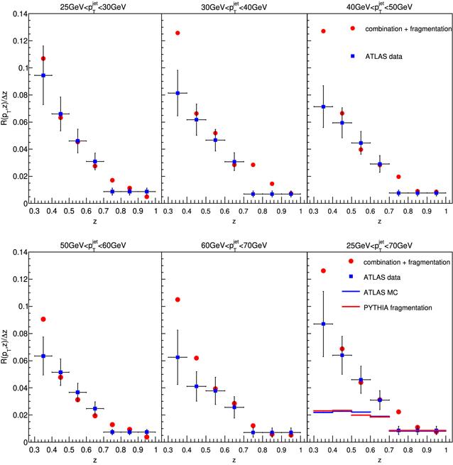
this means that the total cross section includes the fragmentation contribution dσF, the combination contribution dσC, and other high twist contributions which we assume are negligible in this study. As mentioned above, the fragmentation function is calculated by PYTHIA. For dσC, since we can not calculate the combination function $\tilde{F}(\xi ,{\xi }_{l})$, we have to give some physical inputs for it. R(pT, z) is only measured for the region of z > 0.3 by ATLAS [2]. So we first have an extreme try—only considering the charm quark which can not contribute to the data via fragmentation. Say, we only consider the contribution from the zc = pc/pjet < 0.3 after the parton shower. The reason is that the fragmentation always gives a D*± meson with momentum smaller than that of the charm quark. That is, z < zc in the fragmentation process. This conjecture is reasonable since generally a quark and an antiquark with large momentum differences are hard to be combined into a hadron.The distribution of light partons is set to be $P({\xi }_{l})=4{{\rm{e}}}^{-0.1{\xi }_{l}^{2}}$ and the non-zero value of the combinational function is taken to be $\tilde{F}(\xi ,{\xi }_{l})={\xi }^{2}$ with zc < 0.3. The conjecture for the combination function is based on the combination not being sensitive to the concrete value of ξl. The R(pT, z) distribution of the D*± mesons produced from the summation of the fragmentation and combination contributions according to equation (20 ) are shown in figure 3. The data [2] are also plotted. In the full pTjet region with $25\lt {p}_{T}^{{\rm{jet}}}\lt 70\,\mathrm{GeV}$, our results agree with the experimental data. The more detailed comparison in the region of $25\lt {p}_{T}^{{\rm{jet}}}\lt 30\,\mathrm{GeV}$, $30\lt {p}_{T}^{{\rm{jet}}}\lt 40\,\mathrm{GeV}$, $40\lt {p}_{T}^{{\rm{jet}}}\,\lt 50\,\mathrm{GeV}$, $50\lt {p}_{T}^{{\rm{jet}}}\lt 60\,\mathrm{GeV}$ and $60\lt {p}_{T}^{{\rm{jet}}}\lt 70\,\mathrm{GeV}$, is also consistent with the data.

Figure 3. R(pT, z) distribution from the summation of both the combination and fragmentation contributions as equation ( |
In the above calculation, we consider the contribution from the combination mechanism taking effect in the region of small momentum 0 < zc < 0.3. However, from the experimental viewpoint, it is the variable z but not zc that can be measured from the final hadrons D*±. To mimic the real process, we simply model the combination based on the above equations in the following way: we propose a distribution function κ(z) to assign the probability of the combination mechanism. Since the fragmentation mechanism has been tested and applied in various processes, and the theoretical framework is very mature and embedded into the generator, we can get κ(z) by fitting the data. The result is shown in figure 4. Here we extract the probability distribution function κ(z) = λe−λz/(1 − e−λ) with $P({\xi }_{l})={{\rm{e}}}^{-{\xi }_{l}^{2}}$, λ = 4.6. By this way, we can describe the data well.
Figure 4. R(pT, z) distribution from both the combination and fragmentation contributions (red disc) compared to the data (blue square) from the ATLAS [2]. Here the combination probability function is taken as κ(z) = λe−λz/(1 − e−λ) with $P({\xi }_{l})={{\rm{e}}}^{-{\xi }_{l}^{2}}$, λ = 4.6. Since κ(z) has taken the effects of combination probability, $\tilde{F}(\xi ,{\xi }_{l})$ is set to one to avoid the double counting of the combination effects. |
4. Discussion and application
Hadron production at the high energy collision provides plenty of phenomena for the study of QCD. In this paper, we have derived the factorization formula for the D* production in the combination process. As an application, we have summed the combination and fragmentation contributions to compare with the experimental data. With the proper combination function $\tilde{F}(\xi ,{\xi }_{l})$ and the light parton distribution function P(ξl), the calculations are in agreement with the data.
The above investigations demonstrate the importance of the combination mechanism. The experiments which measure the hadron distribution in a jet show the hadronization process is more complex than a simple fragmentation picture, especially the small z distribution. Such a phenomenon is also observed in heavy ion scattering as measuring the jet quenching [18–20]. These two cases share some similarities such as that underlying events are important. If we consider the hadronization process as an effective coupling of the quark degree of freedom with the hadronic one, then the simplest operator relevant is the fragmentation, including two field operators, one of which is the quark field and the other is the hadron. The next one to be considered is the operators including two quark fields and one hadron field. This is the combination contribution. When the combination is taken into account, the density of the partons will make sense, as shown by our formulations above. From this consideration, one can suspect the larger the partonic density, the more the combination contributes. So further measurements in higher energies, as well as multiplicity-triggered events, can give richer phenomenology.
The combination matrix elements are not yet available from data or some non-perturbative calculations, this is why we make a trial in the above section and fit the data by a simple model. It is obvious that with more and more measurements on the processes including combination contribution, one can understand more. On the other hand, the quark (re)combination models have a long history. They can date back to more than three decades ago. From then on, different kinds of quark (re)combination models are presented in application to hadron production in various high energy processes (see, e.g., [21] and references therein). These models work on the quark–gluon degree of freedom as well as the hadronic one.