


Introduction
The effects of a gravitational field produced by topological defects and curved space-time on quantum mechanical systems have been of growing interest among researchers. Topological defects such as cosmic strings [1], global monopole [2] and domain walls [3] have been produced in the early universe during phase transition through a spontaneous symmetry-breaking mechanism. The curved space-times with topological defects have been studied in quantum systems, such as in a cosmic string space-time background [4], in a Gödel and Gödel-type space-times background [5, 6], in a point-like global monopole space-time [2], in a magnetic cosmic string [7] and a magnetic chiral cosmic string space-times background [8] in five dimensions. Many authors have investigated the relativistic quantum dynamics of spin-zero scalar particles (via the Klein–Gordon equation) with external potentials of various kinds (linear, Coulomb- and Cornell-type) in these space-times backgrounds (see, Ref. [9] for details discussion).
Harmonic interactions play an important role in different areas of physics. The harmonic oscillator appears as a model in condensed matter systems, quantum statistical mechanics, quantum field theory and quantum physics. In relativistic quantum mechanics, a well-known version of the harmonic oscillator was first proposed in [10] for spin-1/2 particles called the Dirac oscillator. This relativistic oscillator model was examined by replacing the momentum vector with $\vec{p}\to \left(\vec{p}-{\mathtt{i}}\,m\,\omega \,\vec{r}\right)$ in the wave equation. The Dirac oscillator has been studied in a commutative [10] and non-commutative [11] field theory. Inspired by this Dirac oscillator, a similar oscillator model for spin-zero bosons has been proposed in [12, 13] called the Klein–Gordon oscillator. Later on, several authors have investigated this spin-zero oscillator model in various space-times backgrounds, for instance, with a magnetic field in cosmic string space-time [14], with a coulomb-type scalar [15] and vector potentials [16], with a magnetic field and Cornell-type scalar potential in the Som-Raychaudhuri space-time [17], in the five-dimensional cosmic string space-time, magnetic cosmic string space-time, and magnetic cosmic string space-time with torsion [18], with a linear and Coulomb-type potentials [19], with a Coulomb-type scalar potential in cosmic string space-time [20], in (1 + 2)-dimensional Gürses space-time [21] and with a Coulomb-type potential [22], with a magnetic in the space-time with spacelike dislocation [23], with a magnetic field in cosmic string with spacelike dislocation [24], in cosmic string space-time with a Cornell-type potential [25], in rotating cosmic string space-time with a Cornell-type scalar potential [26], with a magnetic field in the space-time with a spacelike dislocation subject to a linear confining potential [27], with a magnetic field in a non-commutative space [28, 29], with rotating effects in a space-time with magnetic screw dislocation [30], in a topologically non-trivial space-time [31], with a magnetic field in five-dimensional Minkowski space-time with a Cornell-type scalar potential [32], with a magnetic field in five-dimensional cosmic string space-time with a Cornell-type scalar potential [33], in a global monopole space-time [34], in a global monopole spacetime with rainbow gravity [35], under the effects of Lorentz symmetry violation [36–39].
In [31], authors studied a spin-zero relativistic quantum oscillator model under non-inertial effects defined by the rotating frame of reference in a topologically non-trivial space-time without any external fields. They solved the Klein–Gordon oscillator analytically and obtained the eigenvalue solution. They noted that in their analysis, no external magnetic and quantum flux fields were considered. Inspired by this work, we study the same relativistic quantum oscillator system under uniform magnetic and quantum flux fields without any rotational effects in this topologically non-trivial space-time. We solve the Klein–Gordon oscillator analytically and discuss the effects of the non-trivial topology and the external uniform magnetic and quantum flux fields on the energy profile and wave function. We see that the eigenvalue solution is modified by the external magnetic and quantum flux fields in addition to the non-trivial topology of the geometry. Furthermore, the eigenvalue solution depends on the magnetic flux, and this dependence of the eigenvalue on the geometric quantum phase shows an analogue of the Aharonov–Bohm effect [40, 41] for the bound state.
We summarise this paper as follows: in section 2, we will describe a topologically non-trivial space-time geometry, and then determine the solution of the Klein–Gordon oscillator equation in the presence of a uniform magnetic field; and finally conclusions in section 3.
KG-Oscillator under magnetic and quantum flux fields in a topologically non-trivial geometry
In this section, we investigate the relativistic quantum oscillator described by the Klein–Gordon oscillator (KGO) equation [12, 13] in the presence of a uniform magnetic field in a topologically non-trivial space-time geometry. As stated in the introduction, several authors have studied the spin-zero relativistic quantum oscillator model in various space-time backgrounds in quantum systems.
Therefore, the relativistic quantum dynamics of the scalar field is described by the following wave equation (in the system of units where c = 1 = ℏ = G) [9, 17, 20, 23,24, 26, 27, 30, 32–35, 42–47]
$\begin{eqnarray}\left[-\displaystyle \frac{1}{\sqrt{-g}}\,{D}_{\mu }\left\{\sqrt{-g}\,{g}^{\mu \nu }\,{D}_{\nu }\right\}+{M}^{2}\right]\,{\rm{\Psi }}=0,\end{eqnarray}$
where g is the determinant of the metric tensor gμν, $\Psi$ is the wave function, and M is the rest mass of the scalar field. Here, we followed [46] in introducing an electromagnetic four-vector potential Aμ through a minimal substitution ${\partial }_{\mu }\,\to {D}_{\mu }\equiv \left({\partial }_{\mu }-{\mathtt{i}}\,e\,{A}_{\mu }\right)$ in the wave equation, where e is the electric charge. This procedure has been explored in recent studies in quantum mechanical systems by several authors [9, 17, 20, 23, 24, 26, 27, 30, 32–35, 42–45, 47].The space-time produced by a topologically non-trivial geometry is defined by the configuration S1 × R3, where R3 represents the uncompactified space-time directions and S1 is a compactified dimension to a circle of finite radius R (see figure 1). Therefore, the space-time under consideration in the polar coordinates (x0 = t, x1 = r, x2 = φ, x3 = θ) is represented by the following line element [31, 47]
$\begin{eqnarray}{{\mathtt{d}}{s}}^{2}=-{{\mathtt{d}}{t}}^{2}+{{\mathtt{d}}{r}}^{2}+{{r}}^{2}\,{\mathtt{d}}{{\phi }}^{2}+{R}^{2}\,{\mathtt{d}}{{\theta }}^{2},\end{eqnarray}$
where the ranges of the different coordinates are − ∞ < t < +∞ , 0 ≤ r < ∞, φ ∈ [0, 2 π] and 0 ≤ θ < 2 π. For the above space-time geometry, the covariant and the contravariant form of the metric tensor are given by $\begin{eqnarray}{g}_{\mu \nu }=\left(\begin{array}{cccc}-1 & 0 & 0 & 0\\ 0 & 1 & 0 & 0\\ 0 & 0 & {r}^{2} & 0\\ 0 & 0 & 0 & {R}^{2}\end{array}\right),{g}^{\mu \nu }=\left(\begin{array}{cccc}-1 & 0 & 0 & 0\\ 0 & 1 & 0 & 0\\ 0 & 0 & \displaystyle \frac{1}{{r}^{2}} & 0\\ 0 & 0 & 0 & \displaystyle \frac{1}{{R}^{2}}\end{array}\right),\end{eqnarray}$
while the determinant of the above metric tensor gμν is given by $\det \,g=-{r}^{2}\,{R}^{2}$.Now, we insert an oscillator with the scalar field by replacing the radial momentum vector [14–39, 44] as follows:
$\begin{eqnarray}{\partial }_{\mu }\to ({\partial }_{\mu }+M\,\omega \,{X}_{\mu }),\end{eqnarray}$
where ω is the oscillation frequency, and ${X}_{\mu }\,=(0,r,0,0)=r\,{\delta }_{\mu }^{r}$ is a four-vector with r being the distance from the particle to the axis of symmetry. As stated in the introduction, several authors have studied the relativistic quantum oscillator in various space-time backgrounds without and/or with an external magnetic field as well as scalar and vector potential of different kinds.In this way, the Klein–Gordon oscillator from equation (1 ) becomes
$\begin{eqnarray}\begin{array}{l}\left[\displaystyle \frac{-1}{\sqrt{-g}}({D}_{\mu }+M\omega {X}_{\mu })\left\{\sqrt{-g}{g}^{\mu \nu }({D}_{\nu }-M\omega {X}_{\nu })\right\}+{M}^{2}\right]{\rm{\Psi }}\\ \,\,=\,0.\end{array}\end{eqnarray}$
In this work, we have chosen the three-vector potential $\vec{A}$ of the electromagnetic field [9, 17, 23, 24, 27, 30, 42–45, 47] given by
$\begin{eqnarray}{A}_{r}=0={A}_{\theta },\quad {A}_{\phi }=\left(-\displaystyle \frac{1}{2}\,{B}_{0}\,{r}^{2}+\displaystyle \frac{{{\rm{\Phi }}}_{B}}{2\,\pi }\right),\end{eqnarray}$
where ΦB = Φ Φ0 is the magnetic flux which is a constant, Φ is the amount of magnetic flux, and Φ0 = 2 π e−1 is the quantum of magnetic flux. Note that the non-zero component Aφ of the electromagnetic potential can be written as Aφ = Aφ,1 + Aφ,2, where the first part, ${A}_{\phi ,1}=-\tfrac{1}{2}\,{B}_{0}\,{r}^{2},$ only contributes a uniform magnetic field $\vec{B}=\vec{{\rm{\nabla }}}\times \vec{A}\,=(0,0,-{B}_{0})$ and that the second part ${A}_{\phi ,2}=\tfrac{{{\rm{\Phi }}}_{B}}{2\,\pi }$ [23, 24,26, 27, 30, 33, 44, 45] is constant. We will show later on that the energy profiles of the oscillator fields depend on the geometric quantum phase ΦB which gives us the gravitational analogue of the Aharonov–Bohm (AB) effect [40, 41]. This AB effect is a quantum mechanical phenomenon that has been investigated in different branches of physics including quantum systems [9, 18, 23, 24, 26, 30, 32, 33, 43–45, 47].Therefore, the Klein–Gordon oscillator equation (5 ) in the space-time background (2 ) and using equation (6 ) becomes
$\begin{eqnarray}\begin{array}{l}\left[-\displaystyle \frac{{{\mathtt{d}}}^{2}}{{\mathtt{d}}{t}^{2}}+\displaystyle \frac{1}{r}\left(\displaystyle \frac{{\mathtt{d}}}{{\mathtt{d}}r}+M\omega r\right)\left(r\displaystyle \frac{{\mathtt{d}}}{{\mathtt{d}}r}-M\omega {r}^{2}\right)\right.\\ \left.+\,\displaystyle \frac{1}{{r}^{2}}{\left(\displaystyle \frac{{\mathtt{d}}}{{\mathtt{d}}\phi }-{\mathtt{i}}{\rm{\Phi }}+{\mathtt{i}}\,M{\omega }_{c}{r}^{2}\right)}^{2}+\displaystyle \frac{1}{{R}^{2}}\displaystyle \frac{{{\mathtt{d}}}^{2}}{{\mathtt{d}}{\theta }^{2}}\right]{\rm{\Psi }}={M}^{2}{\rm{\Psi }}.\end{array}\end{eqnarray}$
That may be rewritten as $\begin{eqnarray}\begin{array}{l}\left[-\displaystyle \frac{{{\mathtt{d}}}^{2}}{{\mathtt{d}}{t}^{2}}+\displaystyle \frac{{{\mathtt{d}}}^{2}}{{\mathtt{d}}{r}^{2}}+\displaystyle \frac{1}{r}\,\displaystyle \frac{{\mathtt{d}}}{{\mathtt{d}}r}-{M}^{2}\,{\omega }^{2}\,{r}^{2}-2\,M\,\omega \right.\\ \left.+\,\displaystyle \frac{1}{{r}^{2}}{\left(\displaystyle \frac{{\mathtt{d}}}{{\mathtt{d}}\phi }-{\mathtt{i}}\,{\rm{\Phi }}+{\mathtt{i}}M{\omega }_{c}{r}^{2}\right)}^{2}+\displaystyle \frac{1}{{R}^{2}}\displaystyle \frac{{{\mathtt{d}}}^{2}}{{\mathtt{d}}{\theta }^{2}}\right]{\rm{\Psi }}={M}^{2}{\rm{\Psi }}.\end{array}\end{eqnarray}$
Here, we have written ${\omega }_{c}=\tfrac{e\,{B}_{0}}{2\,M}$ called the cyclotron frequency.We chose the following ansatz for the total wave function $\Psi$(t, r, φ, θ) in terms of a radial wave function ψ(r) given by
$\begin{eqnarray}{\rm{\Psi }}(t,r,\phi ,\theta )={{\mathtt{e}}}^{{\mathtt{i}}(-E\,t+l\,\phi +q\,\theta )}\,\psi (r),\end{eqnarray}$
where E is the energy of the scalar field , l = 0, ±1, ±2, …. are the eigenvalues of the angular momentum operator $-{\mathtt{i}}\,{\hat{\partial }}_{\phi }$ and q = 0, ±1, ±2, …. are the eigenvalues of the angular momentum operator $-{\mathtt{i}}\,{\hat{\partial }}_{\theta }$. One can easily show that the total wave function satisfies the following condition $\begin{eqnarray}{\rm{\Psi }}(t,r,\phi ,\theta )={\rm{\Psi }}(t,r,\phi +2\,\pi ,\theta +2\,\pi \,R),\end{eqnarray}$
for given values of l, q.Substituting the wave function (9 ) into equation (8 ), we have11 ) can be rewritten as13 ) is a second order linear homogeneous differential equation which can easily be solved using the well-known Nikiforov-Uvarov method [48, 49].
$\begin{eqnarray}\psi ^{\prime\prime} (r)+\displaystyle \frac{1}{r}\,\psi ^{\prime} (r)+\left({\rm{\Delta }}-{M}^{2}\,{{\rm{\Omega }}}^{2}\,{r}^{2}-\displaystyle \frac{l{{\prime} }^{2}}{{r}^{2}}\right)\psi (r)=0,\end{eqnarray}$
where $l^{\prime} =(l-{\rm{\Phi }})$ and $\begin{eqnarray}\begin{array}{l}{\rm{\Delta }}={E}^{2}-{M}^{2}-2\,M\left(\omega +{\omega }_{c}\,l^{\prime} \right)-\displaystyle \frac{{q}^{2}}{{R}^{2}},\\ {\rm{\Omega }}=\sqrt{{\omega }^{2}+{\omega }_{c}^{2}}.\end{array}\end{eqnarray}$
Let us perform a change of variables via x = M Ω r2. Then, equation ( $\begin{eqnarray}\psi ^{\prime\prime} (x)+\displaystyle \frac{1}{x}\,\psi ^{\prime} (x)+\displaystyle \frac{1}{{x}^{2}}\left(-{\xi }_{1}\,{x}^{2}+{\xi }_{2}\,x-{\xi }_{3}\right)\psi (x)=0,\end{eqnarray}$
where we have defined $\begin{eqnarray}{\xi }_{1}=\displaystyle \frac{1}{4},\quad {\xi }_{2}=\displaystyle \frac{{\rm{\Delta }}}{4\,M\,{\rm{\Omega }}},\quad {\xi }_{3}=\displaystyle \frac{l{{\prime} }^{2}}{4}.\end{eqnarray}$
Equation (The Nikiforov-Uvarov (NU) method is helpful in order to solve the second-order differential equations of physical interest. Several authors have successfully applied this NU method in finding the exact solutions of the wave equations both in the non-relativistic and relativistic limits (e. g., Refs. [21, 22, 35, 47, 50, 51]).
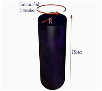
Figure 1. Representation of topologically non-trivial space-time S1 × R3 [31]. |
Thus, by comparing equation (13 ) with equation (A.1) in the appendix in [21, 22], we have
$\begin{eqnarray}\begin{array}{l}{\alpha }_{1}=1,\,\,{\alpha }_{2}=0,\,\,{\alpha }_{3}=0,\,\,{\alpha }_{4}=0,\,\,{\alpha }_{5}=0,\,\,{\alpha }_{6}={\xi }_{1},\\ {\alpha }_{7}=-{\xi }_{2},\,\,{\alpha }_{8}={\xi }_{3},\,\,{\alpha }_{9}={\xi }_{1},\,\,{\alpha }_{10}=1+2\,\sqrt{{\xi }_{3}},\\ {\alpha }_{11}=2\,\sqrt{{\xi }_{1}},\,\,{\alpha }_{12}=\sqrt{{\xi }_{3}},\,\,{\alpha }_{13}=-\sqrt{{\xi }_{1}}.\end{array}\end{eqnarray}$
Using ξ1,…,ξ3 from equation (14 ) and equation (15 ) into equation (A.3) in the appendix in [21, 22], one can obtain the following expression of the energy eigenvalues given by
$\begin{eqnarray}\begin{array}{l}(2\,n+1)\sqrt{{\xi }_{1}}-{\xi }_{2}+2\,\sqrt{{\xi }_{1}\,{\xi }_{3}}=0\\ \Rightarrow \,\,\,\displaystyle \frac{{\rm{\Delta }}}{2\,M\,{\rm{\Omega }}}=(2\,n+1+| l^{\prime} | )\\ \Rightarrow \,\,\,{E}_{n,l,q}=\pm \,\sqrt{{M}^{2}+\sum +{\left(\displaystyle \frac{q}{R}\right)}^{2}},\end{array}\end{eqnarray}$
where n = 0, 1, 2,…. and we have set the parameter ∑ as $\begin{eqnarray}\sum \,=\,2\,M\left\{\omega +{\omega }_{c}\,l^{\prime} +\sqrt{{\omega }^{2}+{\omega }_{c}^{2}}\left(2\,n+1+| l^{\prime} | \right)\right\}.\end{eqnarray}$
We have plotted a few graphs of the energy levels with different parameters, such as the external magnetic field B0 (figures 2–3), the oscillator frequency ω (figures 4–5), and radius R of the compact circle S1 (figures 6–7) for different values of other parameters.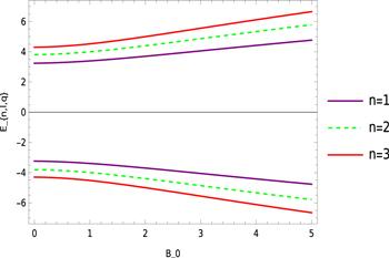
Figure 2. l = 1 = M = q = R = ω = e, Φ = 3/4. |

Figure 3. l = 1 = q = R = M = e, Φ = 1/2. |
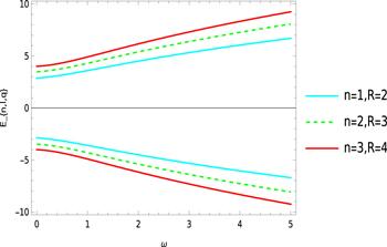
Figure 4. l = 1 = q = M = e, Φ = 3/4, B0 = 2. |
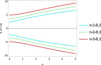
Figure 5. l = 1 = q = R = M = e, Φ = 4/5. |
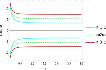
Figure 6. l = 1 = q = M = B0 = e, Φ = 1/2. |
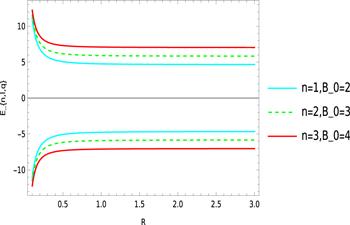
Figure 7. l = 1 = q = M = e, ω = 2, Φ = 1/2. |
The normalized radial wave functions of the quantum system are given by (see appendix for calculation)
$\begin{eqnarray}{\psi }_{n,l}(x)={\left(2\,M\,{\rm{\Omega }}\right)}^{\tfrac{1}{2}}\,\sqrt{\displaystyle \frac{n!}{\left(n+| l^{\prime} | \right)!}}\,{x}^{\tfrac{| l^{\prime} | }{2}}\,{{\mathtt{e}}}^{-\tfrac{x}{2}}\,{{\rm{L}}}_{n}^{(| l^{\prime} | )}(x),\end{eqnarray}$
which depends on the quantum numbers $\left\{n,l,q\right\}$ as well as the magnetic flux which decreases the results. Here ${{\rm{L}}}_{n}^{(\tau )}(\xi )$ is the generalized Laguerre polynomials which is orthogonal over the range (0, ∞ ] w. r. t. weighting function ${{\mathtt{e}}}^{-\xi }\,{{\rm{L}}}_{n}^{(\tau )}(\xi )$ given by $\begin{eqnarray}{\int }_{0}^{\infty }{\xi }^{\tau }\,{{\mathtt{e}}}^{-\xi }\,{{\rm{L}}}_{n}^{(\tau )}(\xi ){{\rm{L}}}_{m}^{(\tau )}(\xi ){\rm{d}}\xi =\left(\displaystyle \frac{(n+\tau )!}{n!}\right){\delta }_{n\,m}.\end{eqnarray}$
We have plotted a few graphs of the normalized wave function ψn,l(x) for different values of the magnetic fields B0, the quantum flux Φ, the oscillator frequency ω, and the quantum numbers {n, l} (figures 8–11).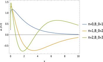
Figure 8. l = 1 = M = ω = e, Φ = 3/4. |
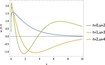
Figure 9. l = 1 = M = B0 = e, Φ = 3/4. |

Figure 10. l = 1 = M = e, ω = 2 = B0. |

Figure 11. n = 1 = M = e = Φ, ω = 2 = B0. |
In terms of r, this normalized radial wave function (18 ) becomes12 ) and ${D}_{n,l}=\sqrt{\tfrac{2(n!)}{(n+| l^{\prime} | )!}}$. Equation (16 ) is the relativistic energy profile and equation (18 ) is the normalized wave function of charged quantum oscillator fields in the presence of a uniform magnetic field in a topologically non-trivial space-time geometry. We can see that the energy profile is modified by the non-trivial topology defined by the radius R of the compact circle, and the external magnetic field B0. Furthermore, we also see that the energy eigenvalues depend on the geometric quantum phase ΦB and is a periodic function of it with a periodicity Φ0, and, we have that, En,l,q(ΦB ± Φ0 τ) =En,l∓τ,q(ΦB), where τ = 0, 1, 2, …. This dependence of the eigenvalues on the geometric quantum phase gives rise to the gravitational analogue of the Aharonov–Bohm effect [40, 41]. We have plotted graphs showing the effects of non-trivial topology and the external uniform magnetic field with quantum flux on the energy eigenvalues En,l,q of the oscillator fields (figure 2).
$\begin{eqnarray}{\psi }_{n,l}(r)={\left(M{\rm{\Omega }}\right)}^{\tfrac{1+| l^{\prime} | }{2}}\,{D}_{n,l}\,{r}^{| l^{\prime} | }\,{{\mathtt{e}}}^{-\tfrac{1}{2}M{\rm{\Omega }}{r}^{2}}{{\rm{L}}}_{n}^{(| l^{\prime} | )}(M{\rm{\Omega }}{r}^{2}),\end{eqnarray}$
where Ω is given in equation (In [31], authors obtained the relativistic energy eigenvalues of quantum oscillator fields in a topologically non-trivial space-time background given by (replacing m → M, n → q, N → n in equation (28) in [31])16 ) reduces to16 ) reduces to21 ) obtained in [31] provided zero magnetic flux field ΦB → 0 here. Thus, we can see that the presented energy eigenvalues equation (16 ) of a relativistic quantum oscillator field becomes further modified by the presence of a uniform magnetic field with magnetic flux in comparison to the previous result obtained in [31]. That's our main motivation in this work, where we can see the effects of the external uniform magnetic and quantum flux fields in addition to the non-trivial topology of the geometry defined by the radius R on the relativistic quantum oscillator fields.
$\begin{eqnarray}{E}_{n,l,q}=\pm \,\sqrt{{M}^{2}+{\left(\displaystyle \frac{q}{R}\right)}^{2}+4\,M\,\omega \left(n+1+\displaystyle \frac{| l| }{2}\right)}.\end{eqnarray}$
For zero magnetic flux ΦB → 0, the relativistic energy eigenvalue of the oscillator fields equation ( $\begin{eqnarray}\begin{array}{l}{E}_{n,l,q}^{2}={M}^{2}+{\left(\displaystyle \frac{q}{R}\right)}^{2}\\ \,+\,2\,M\left\{\omega +{\omega }_{c}\,l+\sqrt{{\omega }^{2}+{\omega }_{c}^{2}}\left(2\,n+1+| l| \right)\right\}.\end{array}\end{eqnarray}$
On the other hand, in absence of external magnetic field B0 → 0, i. e., ωc → 0, the relativistic energy eigenvalue of the oscillator fields equation ( $\begin{eqnarray}{E}_{n,l,q}=\pm \,\sqrt{{M}^{2}+{\left(\displaystyle \frac{q}{R}\right)}^{2}+4\,M\,\omega \left(n+1+\displaystyle \frac{| l-{\rm{\Phi }}| }{2}\right)}\end{eqnarray}$
which is similar to the result (Persistent currents, and magnetization & magnetic susceptibility at zero temperature
In this section, we are interested in analyzing the persistent currents, the magnetization and magnetic susceptibility at zero temperature.
Persistent currents
It is well-known in condensed matter physics [52–54] that the dependence of the energy eigenvalue on the geometric quantum phase gives rise to persistent currents. The expression for the total persistent currents at zero temperature T = 0 is given by [55–57]
$\begin{eqnarray}I=\displaystyle \sum _{n,l,q}\,{I}_{n,l,q}\quad {\rm{and}}\quad {I}_{n,l,q}=-\displaystyle \frac{{\mathtt{d}}{E}_{n,l,q}}{{\mathtt{d}}{{\rm{\Phi }}}_{B}}\end{eqnarray}$
is called the Byers-Yang relation [52].Using the expression equation (16 ), we have the Byers-Yang relation given by
$\begin{eqnarray}\begin{array}{rcl}{I}_{n,l,q} & = & \pm \,\displaystyle \frac{\left(e\,{B}_{0}+\sqrt{4\,{M}^{2}\,{\omega }^{2}+{e}^{2}\,{B}_{0}^{2}}\right)}{2\,{{\rm{\Phi }}}_{0}}\\ & & \times \,\displaystyle \frac{1}{\sqrt{{M}^{2}+\sum +{\left(\tfrac{q}{R}\right)}^{2}}}.\end{array}\end{eqnarray}$
One can see from (25 ) that the persistent currents are influenced by the non-trivial topology of the geometry defined by the radius R of the circle S1, the oscillator frequency ω, and the external magnetic field B0 which modified the result.
Magnetization at zero temperature
For the present system, we have the magnetization expression
$\begin{eqnarray}{M}_{n,l,q}({B}_{0},{{\rm{\Phi }}}_{B})=\mp \,\displaystyle \frac{e\left[l^{\prime} +\tfrac{Y\,{\omega }_{c}}{\sqrt{{\omega }^{2}+{\omega }_{c}^{2}}}\right]}{2\,\sqrt{{M}^{2}+\sum +{\left(\tfrac{q}{R}\right)}^{2}}},\end{eqnarray}$
where $Y=(2\,n+1+| l^{\prime} | )$.One can see from (27 ) that the magnetization of the quantum system is influenced by the non-trivial topology of the geometry defined by the radius R of the circle S1, the oscillator frequency ω, and the quantum flux field with a magnetic field. Also, its value changes with a change in the quantum numbers {n, l, q}.
Magnetic susceptibility at zero temperature
For the present system, it is given by
$\begin{eqnarray}\begin{array}{l}{\chi }_{n,l,q}=\pm \,\displaystyle \frac{\tfrac{{e}^{2}}{4}{\left[l^{\prime} +\tfrac{Y\,{\omega }_{c}}{\sqrt{{\omega }^{2}+{\omega }_{c}^{2}}}\right]}^{2}}{{\left[{M}^{2}+\sum +{\left(\tfrac{q}{R}\right)}^{2}\right]}^{\tfrac{3}{2}}}\\ \,\,\mp \displaystyle \frac{Y\,{e}^{2}\,{\omega }^{2}}{4\,M{\left({\omega }^{2}+{\omega }_{c}^{2}\right)}^{3/2}\,\sqrt{{M}^{2}+\sum +{\left(\tfrac{q}{R}\right)}^{2}}}.\end{array}\end{eqnarray}$
One can see from (29 ) that the magnetic susceptibility of the quantum system is influenced by the non-trivial topology of the geometry defined by the radius R of the circle S1, the oscillator frequency ω, and the quantum flux field ΦB in addition to the magnetic field. Also, its value changes with a change in the quantum numbers {n, l, q}.
Conclusions
In this analysis, the relativistic quantum motions of the spin-zero oscillator field (via the Klein–Gordon oscillator equation) in the presence of a uniform magnetic field and quantum flux in a topologically non-trivial space-time are studied. The external magnetic field is introduced through a minimal substitution ${\partial }_{\mu }\to {D}_{\mu }\equiv \left({\partial }_{\mu }-{\mathtt{i}}\,e\,{A}_{\mu }\right)$ in the wave equation. Afterwards, we examined the Klein–Gordon oscillator by replacing the radial momentum vector ${p}_{\mu }\to \left({p}_{\mu }+M\,\omega \,r\,{\delta }_{\mu }^{r}\right)$ in the wave equation, where ω is the oscillation frequency. The above radial momentum transformation can also be written as $\tfrac{1}{r}\,\tfrac{\partial }{\partial \,r}\left(r\,\tfrac{\partial }{\partial \,r}\right)\,\to \tfrac{1}{r}\left(\tfrac{\partial }{\partial \,r}+M\,\omega \,r\right)\left(r\,\tfrac{\partial }{\partial \,r}-M\,\omega \,{r}^{2}\right)$ in the cylindrical systems. By choosing a suitable ansatz for the total wave function $\Psi$(t, r, φ, θ), we have derived the radial wave equation of the Klein–Gordon oscillator. We see that this radial wave equation is a homogeneous second-order differential equation which can be solved by the well-known Nikiforov-Uvarov (NU) method. We have used this NU method and obtained the energy eigenvalues given by equation (16 ) and the normalized wave function by equation (18 ) of the relativistic quantum oscillator fields. We have seen that the energy profile of the oscillator fields is modified by the non-trivial topology of the space-time geometry defined by the radius R of the compactified dimension S1 and the external uniform magnetic with quantum flux fields. We have shown that the presented energy eigenvalue gets modified in comparison to the result obtained in [31] due to the presence of uniform magnetic and quantum flux fields in the quantum system.
Furthermore, we have observed that the presented energy eigenvalue depends on the geometric quantum phases ΦB and is a periodic function of it. Thus, we have that, En,l,q(ΦB ± Φ0 τ) = En,l∓τ,q(ΦB), where τ = 0, 1, 2, … This dependence of the energy eigenvalue on the geometric quantum phase gives us the gravitational analogue of the Aharonov–Bohm effect [40, 41]. In addition, we have studied the magnetic properties of the quantum system at Zero temperature, such as persistent currents given by equation (25 ) that arise due to the dependence of the eigenvalue on the geometric quantum phase, the magnetization given by equation (27 ) and the magnetic susceptibility by equation (29 ) in a state defined by the quantum numbers {n, l, q}. We have seen that the non-trivial topology of the geometry is defined by the radius R of the circle S1, the oscillator frequency ω and the external magnetic B0, and quantum flux ΦB fields influence the magnetic parameters. It is worth mentioning that at finite temperature T ≠ 0, one can calculate the partition function $Z(\beta )={\sum }_{n=0}\,{{\mathtt{e}}}^{-\beta \,{E}_{n,l,q}}$ using the compact energy expression equation (16 ), where $\beta =\tfrac{1}{\kappa \,T}$ and κ is the Boltzmann constant. Then using this partition function, the thermodynamic properties of the quantum system, such as the vibrational free energy, mean energy, specific heat capacity, and entropy can be obtained. In addition, one can study the magnetic properties, such as the magnetization, magnetic susceptibility, and persistent currents at finite temperature T ≠ 0 using this partition function as done in [56, 57] which we will do in future work.
This paper aimed to investigate the quantum motions of scalar particles interacting harmonically with a non-trivial topological space-time background with configuration R3 × S1 via the Klein–Gordon oscillator, where the circle S1 is a compactified dimension. We determine how the non-trivial topology of the geometry and the external magnetic and quantum flux fields modify the energy levels and the wave functions of the oscillator fields. We have seen that there is a perturbation in the energy levels and this harmonic interaction would be used for the simulation of various physical systems, such as the vibrational spectrum of a diatomic molecule [58], the binding of heavy quarks [59, 60], the quark–antiquark interaction [61], and the quantum dynamics in Hall droplets of finite size [62] and with harmonic confinement of electrons [63]. From the observational point of view, it is clear that for an observable perturbation in the energy levels, we need a large number of particles in the states, otherwise, the magnitude of the effect on the original spectrum may not enough to be observed.
Thus, we have shown some results for quantum systems where the relativistic effects are taken. With these, it is possible to have an idea about the general aspects of the behaviour of spin-zero scalar fields in a topologically non-trivial space-time where a uniform magnetic field and the magnetic quantum flux exist. Furthermore, in this analysis the gravitational analogue of the Aharonov–Bohm effect [40, 41] is observed because there is a shift in the angular quantum number $l\to l^{\prime} =\left(l-\tfrac{e\,{{\rm{\Phi }}}_{B}}{2\,\pi }\right)$. This is a fundamental subject in physics and the connections between these theories are not yet well understood.
Acknowledgments
We sincerely acknowledged the anonymous kind referee(s) for valuable remarks and helpful suggestions.
Data availability
All data are included in this manuscript.
Conflict of interest
There is no conflict of interest regarding the publication of this manuscript.
Appendix A. Calculation of the normalization constant Nn,l
The normalized radial functions using equation (15 ) into the equation (A.2) in the appendix in [21, 22] are given by
$\begin{eqnarray}{\psi }_{n,l}(x)={N}_{n,l}\,{x}^{\tfrac{| l^{\prime} | }{2}}\,{{\mathtt{e}}}^{-x}\,{{\rm{L}}}_{n}^{(| l^{\prime} | )}(x),\end{eqnarray}$
where Nn,l is the normalization which will determine now.Since equation (13 ) is achieved from equation (11 ) by substituting x = M Ω r2. Thus, we substitute now x = M Ω r2 into the equation (A1 ), and we have the following form of the radial wave function
$\begin{eqnarray}{\psi }_{n,l}(r)={N}_{n,l}{\left(M\,{\rm{\Omega }}\,{r}^{2}\right)}^{\tfrac{| l^{\prime} | }{2}}\,{{\mathtt{e}}}^{-\tfrac{1}{2}\,M\,{\rm{\Omega }}\,{r}^{2}}\,{{\rm{L}}}_{n}^{(| l^{\prime} | )}(M\,{\rm{\Omega }}\,{r}^{2}).\end{eqnarray}$
The normalized total wave function of the quantum system can be expressed as10 ) and ${\int }_{0}^{2\,\pi \,R}{\left(\tfrac{{{\mathtt{e}}}^{{\mathtt{i}}\,q\,\theta }}{R\,\sqrt{2\,\pi }}\right)}^{\dagger }\left(\tfrac{{{\mathtt{e}}}^{{\mathtt{i}}\,q\,\theta }}{R\,\sqrt{2\,\pi }}\right)R\,d\theta =1$.
$\begin{eqnarray}{{\rm{\Psi }}}_{n,l,q}(t,r,\phi ,\theta )={{\mathtt{e}}}^{-{\mathtt{i}}\,{E}_{n,l,q}\,t}\left(\displaystyle \frac{{{\mathtt{e}}}^{{\mathtt{i}}\,l\,\phi }}{\sqrt{2\,\pi }}\right)\left(\displaystyle \frac{{{\mathtt{e}}}^{{\mathtt{i}}\,q\,\theta }}{R\,\sqrt{2\,\pi }}\right){\psi }_{n,l}(r),\end{eqnarray}$
because the wave function $\Psi$(t, r, φ, θ) satisfies the condition (In literature, the normalization condition is given by
$\begin{eqnarray}{\int }_{V}{{\rm{\Psi }}}_{n,l,q}^{\dagger }\,{{\rm{\Psi }}}_{m,l,q}\,d\tau ={\delta }_{n\,m},\end{eqnarray}$
where dτ = dr(r dφ)(R dθ) is the volume element for the present system of coordinates.Thereby, substituting (A3 ) and (A2 ) into the equation (A4 ), we haveA2 ), one will get the result (20 ).
$\begin{eqnarray}\begin{array}{ll} & R\,| {N}_{n,l}{| }^{2}\left[\displaystyle \frac{1}{2\,\pi }\right]\left[\displaystyle \frac{1}{2\,\pi \,{R}^{2}}\right]\\ & \times \,{\int }_{V}{\left(M\,{\rm{\Omega }}\,{r}^{2}\right)}^{| l^{\prime} | }\,{{\mathtt{e}}}^{-M\,{\rm{\Omega }}\,{r}^{2}}{\left[{L}_{n}^{(| l^{\prime} | )}(M\,{\rm{\Omega }}\,{r}^{2})\right]}^{2}\\ & \times \,r\,{\rm{d}}{r}\,{\rm{d}}\phi \,{\rm{d}}\theta =1\\ \Rightarrow & | {N}_{n,l}{| }^{2}\,\displaystyle \frac{1}{2\,M\,{\rm{\Omega }}}\\ & \times \,{\int }_{0}^{\infty }{\rm{d}}(M\,{\rm{\Omega }}\,{r}^{2}){\left(M{\rm{\Omega }}\,{r}^{2}\right)}^{| l^{\prime} | }{{\mathtt{e}}}^{-M\,{\rm{\Omega }}\,{r}^{2}}\\ & \times {\left[{L}_{n}^{(| l^{\prime} | )}(M{\rm{\Omega }}\,{r}^{2})\right]}^{2}=1\\ \Rightarrow & | {N}_{n,l}{| }^{2}\,{\int }_{0}^{\infty }{dx}\,{x}^{| l^{\prime} | }\,{{\mathtt{e}}}^{-x}{\left[{L}_{n}^{(| l^{\prime} | )}(x)\right]}^{2}=2\,M\,{\rm{\Omega }}\\ \Rightarrow & | {N}_{n,l}{| }^{2}\,\displaystyle \frac{(n+| l^{\prime} | )!}{n!}=2\,M\,{\rm{\Omega }}\quad ({\rm{using\; equation}}(19))\\ \Rightarrow & {N}_{n,l}={\left(M\,{\rm{\Omega }}\right)}^{\tfrac{1}{2}}\,\sqrt{\displaystyle \frac{2(n!)}{(n+| l^{\prime} | )!}}.\end{array}\end{eqnarray}$
Therefore, by substituting Nn,l into the equation (