


1. Introduction
Nuclear matter space distribution can be approximately described by nuclear shape, which is one of the most important and fundamental physical quantities in nuclear-structure research. Indeed, it is well known that the nuclear shape plays an important role in understanding various nuclear phenomena. Moreover, it is to some extent crucial for understanding the nucleon−nucleon interaction responsible for microscopic nuclear structure. Both the ground state and dynamical properties of nuclei are shape-dependent. In heavy-ion reaction dynamics, the nuclear shape is also revealed to play important roles [1–3]. In practice, the nuclear shape is usually expressed by a set of deformation parameters (e.g. the collective coordinates αλμ in the expansion of spherical harmonics). The measurements of nuclear shape (namely, such a set of deformation parameters) are of importance for understanding nuclear properties and even checking nuclear structure models. Experimentally, some nuclear deformations are usually determined by scattering measurements (e.g. electron [4], proton [5], neutron [6], deuteron [7], 3He [8], and α scattering [9]), Coulomb excitation [10], heavy ions [11], muonic X-rays [12] and so on. Theoretical estimates usually come from equilibrium deformation predictions given by macroscopic−microscopic Strutinsky-type calculations with phenomenological one-body nuclear potential [e.g. the frequently used Nilsson or Woods−Saxon (WS) potentials] or by microscopic self-consistent Hartree–Fock calculations with effective two-body nucleon−nucleon interactions (e.g. the Skyrme or Gogny nuclear forces). The ground-state shapes have been systematically studied by different methods, cf [13–17].
The lower-order and reflection-symmetric shape degrees of freedom (e.g. α2μ and α4μ) are expected to be of importance since the other ones only affect a relatively small percentage of all nuclei [18]. Needless to say, the axial quadrupole deformation β2 is the most important and is generally sufficient to explain most nuclear phenomena. It has also been pointed out that some unexpected characteristics, such as wobbling, signature splitting (or inversion), and chiral doublets, may be caused by γ deformation [19–21]. An empirical formula of energy staggering in a γ band was suggested by Zamfir and Casten [22] to indicate the triaxiality in nuclei. In addition, the importance of the hexadecapole deformation β4 becomes non-negligible in e.g. the rare-earth and actinide regions [23].
Relative to the quadrupole deformation β2, the hexadecapole deformation is difficult to determine experimentally with good precision, primarily because of its small magnitude [1, 24]. Furthermore, all the results are model dependent and quite different with big uncertainties [25]. However, with the development of techniques and tactical skills, the bottleneck is being or will be broken. For instance, the hexadecapole nuclear deformations have been accurately measured by scattering of α particles at energies well above the Coulomb barrier for rare-earth nuclei [26]. A systematic variation of β4 from positive in the light rare earths to negative in the heavy ones has been revealed [26] through excitation of the ground rotational band by 50 MeV α particles. The evidence for hexadecapole collectivity in closed-shell nuclei was presented by examining the observed characteristics of the lowest 4+ excited state [27]. In the lanthanide nuclei, it is found that the β4 deformation drops from large positive values around +0.1 to large negative values around −0.1 as the mass number A increases from 152 to 180 [25]. The β4 measurements are indeed attracting much interest in research on nuclear shape. Recently, Gupta et al [1] determined the hexadecapole β4 deformation of the light-mass nucleus 24Mg using quasi-elastic scattering measurements.
Very recently, across the whole nuclear chart, we performed a systematic β4 calculation [28], in which several β4 deformation islands were found, agreeing with the results in [16] but including the results under rotation. In this study, we mainly focus on the effects of the axial and nonaxial but reflection-symmetric hexadecapole deformation degrees of freedom (e.g. α40, α42 and α44) on nuclear structure in the A = 230 nuclear region, where the large hexadecapole deformation island was identified both theoretically and experimentally [16, 28]. Prior to the present study, we have investigated axial quadrupole and octupole deformations, triaxial deformation, and the corresponding stiffness in some nuclei [29–35] using potential-energy-surface and total-Routhian-surface calculations, which to a large extent help us to convince ourselves of the validity and correctness of our work.
The paper is organized as follows. In the next section, we summarize the principle of the calculations, with a brief description of the PES method. The results of the calculation and discussion are presented in the section that then follows. The final section gives a brief summary and outlook.
2. Theoretical method
In this section, we recall the unified procedure and give the necessary references on our adopted theoretical method, which are helpful to clarify some details for the general reader (e.g. the various variants of the pairing-energy contribution in the macroscopic−microscopic nuclear-structure models [16, 36]). In this project, we perform the present investigation using the potential-energy-surface method, which is widely used and powerful for studying nuclear structure properties. The usual expression for the total energy reads [cf [37] and references therein]
$\begin{eqnarray}\begin{array}{l}{E}^{\omega }(Z,N,\hat{\beta })={E}_{\mathrm{LD}}(Z,N,\hat{\beta })\\ \quad +\delta {E}_{\mathrm{shell}}(Z,N,\hat{\beta })+\delta {E}_{\mathrm{pair}}(Z,N,\hat{\beta }).\end{array}\end{eqnarray}$
The terms ${E}_{\mathrm{LD}}(Z,N,\hat{\beta })$, $\delta {E}_{\mathrm{shell}}(Z,N,\hat{\beta })$ and $\delta {E}_{\mathrm{pair}}(Z,N,\hat{\beta })$ represent the macroscopic liquid-drop energy, the quantum shell correction and the pairing-energy contribution, respectively.In the literature, the adopted phenomenological liquid-drop (LD) models generally include the standard LD model [38], finite-range droplet model [16], Lublin−Strasbourg drop model [39], and so on. These macroscopic models with slight differences can describe the smoothly varying energy, in which the dominating terms are mainly associated with the volume energy, the surface energy, and the Coulomb energy. In this work, the macroscopic energy is obtained from the standard LD model with the parameters used by Myers and Swiatecki [38, 40]. As mentioned in section V in [40], it needs to be stressed that the potential energy relative to the energy of a spherical liquid drop is adopted in the potential-energy-surface calculations (at this moment, one cannot compare with the binding energy of the nucleus between experiment and theory).
The microscopic energies are calculated based on the single-particle levels which are obtained by solving numerically the Schrödinger equation with a phenomenological one-body mean field or self-consistent one. Here, we adopt the realistic WS Hamiltonian [41], as seen below:4 ) due to the different radius parameter. With the WS potential model, one can calculate the WS Hamiltonian matrix by e.g. numerical integral with the aid of a set of orthogonal complete bases. The model parameters (taken from [42, 45]) of the Hamiltonian are usually obtained by the inverse problem theory or χ2-fitting procedure (e.g. fitting the experimental single-particle levels) and can often be adopted for the present mass region (e.g. cf [17]). In this work, we use the eigenfunctions of the axially deformed harmonic oscillator potential in the cylindrical coordinate system as the basis function, as seen below:
$\begin{eqnarray}\begin{array}{rcl}{H}_{\mathrm{WS}} & = & T+{V}_{\mathrm{cent}}(\vec{r};\hat{\beta })+{V}_{\mathrm{so}}(\vec{r},\vec{p},\vec{s};\hat{\beta })\\ & & +{V}_{\mathrm{Coul}}(\vec{r},\hat{\beta }),\end{array}\end{eqnarray}$
where the Coulomb potential ${V}_{\mathrm{Coul}}(\vec{r},\hat{\beta })$, defined as a classical electrostatic potential of a uniformly charged drop, is added for protons. The central part of the WS potential reads $\begin{eqnarray}{V}_{\mathrm{cent}}(\vec{r},\hat{\beta })=\displaystyle \frac{{V}_{0}[1\pm \kappa (N-Z)/(N+Z)]}{1+\exp [{\mathrm{dist}}_{{\rm{\Sigma }}}(\vec{r},\hat{\beta })/a]},\end{eqnarray}$
where the plus and minus signs hold for protons and neutrons, respectively, and the parameter a denotes the diffuseness of the nuclear surface. The term ${\mathrm{dist}}_{{\rm{\Sigma }}}(\vec{r},\hat{\beta })$ represents the distance of a point $\vec{r}$ from the nuclear surface Σ parametrized in terms of the multipole expansion of spherical harmonics Yλμ(θ, φ) (which are convenient to describe the geometrical properties), that is, $\begin{eqnarray}{\rm{\Sigma }}:R(\theta ,\phi )={r}_{0}{A}^{1/3}c(\hat{\beta })\left[1+\displaystyle \sum _{\lambda }\displaystyle \sum _{\mu =-\lambda }^{+\lambda }{\alpha }_{\lambda \mu }{Y}_{\lambda \mu }(\theta ,\phi )\right],\end{eqnarray}$
where the function $c(\hat{\beta })$ ensures the conservation of the nuclear volume and $\hat{\beta }$ denotes the set of all the deformation parameters. In the present work, the shape parametrization considers quadrupole and hexadecapole degrees of freedom, including nonaxial deformations [that is, $\hat{\beta }$ ≡(α20, α2±2, α40, α4±2, α4±4)]. The distance of any point on the nuclear surface from the origin of the coordinate system is denoted by R(θ, φ). Generally speaking, the nucleus prefers to possess x − y, y − z, and x − z plane symmetries. In this case, only the even λ and even μ components are retained. After requesting the hexadecapole degrees of freedom to be functions of the scalars in the quadrupole tensor α2μ, one can reduce the number of independent coefficients to three, namely, β2, γ, and β4, which obey the relationships [42] $\begin{eqnarray}\left\{\begin{array}{l}{\alpha }_{20}={\beta }_{2}\cos \gamma \\ {\alpha }_{22}={\alpha }_{2-2}=-\displaystyle \frac{1}{\sqrt{2}}{\beta }_{2}\sin \gamma \\ {\alpha }_{40}=\displaystyle \frac{1}{6}{\beta }_{4}(5{\cos }^{2}\gamma +1)\\ {\alpha }_{42}={\alpha }_{4-2}=-\displaystyle \frac{1}{12}\sqrt{30}{\beta }_{4}\sin 2\gamma \\ {\alpha }_{44}={\alpha }_{4-4}=\displaystyle \frac{1}{12}\sqrt{70}{\beta }_{4}{\sin }^{2}\gamma .\end{array}\right.\end{eqnarray}$
The (β2, γ, β4) parametrization has all the symmetry properties of Bohr's (β2, γ) parametrization [43, 44]. The spin−orbit potential, which can strongly affect the level order, is defined by $\begin{eqnarray}\begin{array}{l}{V}_{\mathrm{so}}(\vec{r},\vec{p},\vec{s};\hat{\beta })=-\lambda {\left[\displaystyle \frac{{\hslash }}{2{mc}}\right]}^{2}\\ \quad \times \left\{{\rm{\nabla }}\displaystyle \frac{{V}_{0}[1\pm \kappa (N-Z)/(N+Z)]}{1+\exp [{\mathrm{dist}}_{{{\rm{\Sigma }}}_{{so}}}(\vec{r},\hat{\beta })/{a}_{{so}}]}\right\}\times \vec{p}\cdot \vec{s},\end{array}\end{eqnarray}$
where λ denotes the strength parameter of the effective spin−orbit force acting on the individual nucleons. The new surface Σso is different from the one in equation ( $\begin{eqnarray}| {n}_{\rho }{n}_{z}{\rm{\Lambda }}{\rm{\Sigma }}\rangle ={\psi }_{{n}_{\rho }}^{{\rm{\Lambda }}}(\rho ){\psi }_{{n}_{z}}(z){\psi }_{{\rm{\Lambda }}}(\varphi )\chi ({\rm{\Sigma }}).\end{eqnarray}$
For more details, one can see e.g. [46]. During the calculation, the eigenfunctions with the principal quantum numbers N ≤ 12 and 14 are chosen as the basis set for protons and neutrons, respectively. It is found that, via such a basis cutoff, the results are sufficiently stable with respect to a possible enlargement of the basis space, indicating the completeness to some extent. In addition, the time reversal (resulting in the Kramers degeneracy) and spatial symmetries (e.g. the existence of three symmetry planes mentioned above) are used for simplifying the calculations of the Hamiltonian matrix.The shell correction $\delta {E}_{\mathrm{shell}}(Z,N,\hat{\beta })$, as seen in equation (1 ), which is usually the most important correction to the LD energy, can be calculated by the Strutinsky method,
$\begin{eqnarray}\delta {E}_{\mathrm{shell}}(Z,N,\hat{\beta })=\sum {e}_{i}-\int e\tilde{g}(e){\rm{d}}e,\end{eqnarray}$
where ei denotes the calculated single-particle levels and $\tilde{g}(e)$ is the so-called smooth level density. Obviously, the smooth level distribution function is the most important quantity, which was earlier defined as $\begin{eqnarray}\tilde{g}(e,\gamma )\equiv \displaystyle \frac{1}{\gamma \sqrt{\pi }}\displaystyle \sum _{i}\exp \left[-\displaystyle \frac{{\left(e-{e}_{i}\right)}^{2}}{{\gamma }^{2}}\right],\end{eqnarray}$
where γ denotes the smoothing parameter without much physical significance. To eliminate any possibly strong γ-parameter dependence for the calculated result, the mathematical form of the smooth level density $\tilde{g}(e)$ is optimized by introducing a phenomenological curvature-correction polynomial Pp(x) [40, 47–49], $\begin{eqnarray}\begin{array}{l}\tilde{g}(e,\gamma ,p)=\displaystyle \frac{1}{\gamma \sqrt{\pi }}\displaystyle \sum _{i=1}{P}_{p}\left(\displaystyle \frac{e-{e}_{i}}{\gamma }\right)\\ \quad \times \exp \left[-\displaystyle \frac{{\left(e-{e}_{i}\right)}^{2}}{{\gamma }^{2}}\right].\end{array}\end{eqnarray}$
The corrective polynomial Pp(x) can be expanded in terms of the Hermite or Laguerre polynomials. The corresponding coefficients of the expansion can be obtained using the orthogonality properties of these polynomials and the Strutinsky condition [50]. So far, some other methods have also been developed for calculating microscopic shell correction, e.g. the semiclassical Wigner−Kirkwood expansion method [42, 51] and the Green function method [52]. In this work, we adopt the widely used Strutinsky method despite its known problems that appear for mean-field potentials of finite depth as well as for nuclei close to the proton or neutron drip lines. The smooth level density is calculated with a sixth-order Hermite polynomial and a smoothing parameter γ = 1.20ℏω0, where ℏω0 = 41/A1/3 MeV [40].Another important single-particle correction, besides the shell correction, is the pairing-energy contribution. As is well known, because of the short-range interaction of nucleon pairs in time-reversed orbitals, the total potential energy relative to the energy without pairing in a nucleus is always reduced. There exist various variants of the pairing-energy contribution in microscopic-energy calculations, as was recently pointed out in [53]. Typically, several kinds of phenomenological pairing energy expressions (namely, pairing correlation and pairing correction energies employing or not employing the particle number projection technique) are widely adopted in applications of the macroscopic−microscopic approach [53]. In the present work, the contribution $\delta {E}_{\mathrm{pair}}(Z,N,\hat{\beta })$ in equation (1 ) is the pairing correlation energy. The pairing is treated by the Lipkin−Nogami (LN) method [54], which helps avoid not only the spurious pairing phase transition but also the particle number fluctuation encountered in the simpler BCS calculation. In the LN technique [54, 55], it aims to minimize the expectation value of the following model Hamiltonian:
$\begin{eqnarray}\hat{{ \mathcal H }}={\hat{H}}_{\mathrm{WS}}+{\hat{H}}_{\mathrm{pair}}-{\lambda }_{1}\hat{N}-{\lambda }_{2}{\hat{N}}^{2}.\end{eqnarray}$
Here, ${\hat{H}}_{\mathrm{pair}}$ indicates the pairing interaction Hamiltonian [56, 57]. The pairing strength is determined by the average gap method [57]. The pairing window, including dozens of single-particle levels, and the respective states (e.g. half of the particle number Z or N) just below and above the Fermi energy, is adopted empirically for both protons and neutrons. The pairing gap Δ, Fermi energy λ [namely, λ1 + 2λ2(Ntotal + 1)], particle number fluctuation constant λ2, occupation amplitudes vk, and shifted single-particle energies ϵk can be determined from the following 2(N2 − N1) + 5 coupled nonlinear equations [54, 57]: $\begin{eqnarray}\left\{\begin{array}{l}{N}_{\mathrm{total}}=2{\sum }_{k={N}_{1}}^{{N}_{2}}{v}_{k}^{2}+2({N}_{1}-1),\\ {\rm{\Delta }}=G{\sum }_{k={N}_{1}}^{{N}_{2}}{u}_{k}{v}_{k},\\ {v}_{k}^{2}=\displaystyle \frac{1}{2}\left[1-\displaystyle \frac{{\varepsilon }_{k}-\lambda }{\sqrt{{\left({\varepsilon }_{k}-\lambda \right)}^{2}+{{\rm{\Delta }}}^{2}}}\right],\\ {\varepsilon }_{k}={e}_{k}+(4\lambda -G){v}_{k}^{2},\\ {\lambda }_{2}=\displaystyle \frac{G}{4}\left[\displaystyle \frac{\left({\sum }_{k={N}_{1}}^{{N}_{2}}{u}_{k}^{3}{v}_{k}\right)\left({\sum }_{k={N}_{1}}^{{N}_{2}}{u}_{k}{v}_{k}^{3}\right)-{\sum }_{k={N}_{1}}^{{N}_{2}}{u}_{k}^{4}{v}_{k}^{4}}{{\left({\sum }_{k={N}_{1}}^{{N}_{2}}{u}_{k}^{2}{v}_{k}^{2}\right)}^{2}-{\sum }_{k={N}_{1}}^{{N}_{2}}{u}_{k}^{4}{v}_{k}^{4}}\right],\end{array}\right.\end{eqnarray}$
where ${u}_{k}^{2}=1-{v}_{k}^{2}$ and k = N1, N1 + 1, ⋯ ,N2. The LN pairing energy for the system of even–even nuclei at the ‘paired solution' (pairing gap Δ ≠ 0) is given by [16, 54] $\begin{eqnarray}\begin{array}{rcl}{E}_{\mathrm{LN}} & = & \displaystyle \sum _{k}2{{v}_{k}}^{2}{e}_{k}-\displaystyle \frac{{{\rm{\Delta }}}^{2}}{G}-G\displaystyle \sum _{k}{{v}_{k}}^{4}\\ & & -4{\lambda }_{2}\displaystyle \sum _{k}{{u}_{k}}^{2}{{v}_{k}}^{2},\end{array}\end{eqnarray}$
where ${{v}_{k}}^{2}$, ek, Δ and λ2 represent the occupation probabilities, single-particle energies, pairing gap and number-fluctuation constant, respectively. Correspondingly, the partner expression at the ‘no-pairing solution' (Δ = 0) reads $\begin{eqnarray}{E}_{\mathrm{LN}}({\rm{\Delta }}=0)=\displaystyle \sum _{k}2{e}_{k}-G\displaystyle \frac{N}{2}.\end{eqnarray}$
The pairing correlation is defined as the difference between paired solution ${E}_{\mathrm{LN}}$ and no-pairing solution ${E}_{\mathrm{LN}}$(Δ = 0).As mentioned in [58], after performing the several standard steps, the total energy can be obtained at each sampling deformation grid. Further, the smooth potential-energy surface/map is able to be given with the help of the interpolation techniques, e.g. a cubic spline function, and then the equilibrium deformations and other physical quantities at such a shape can be determined. Note that different parametrizations generate similar equilibrium deformations in the stiff nuclei. In the soft nuclei, the so-called equilibrium deformations, which may sensitively depend on the model parameters, are meaningless and the dynamic deformations should, in principle, be taken into account.
3. Results and discussion
The calculation of the potential-energy surface is very helpful for understanding the structure properties from different deformation degrees of freedom in nuclei. We perform realistic total energy calculations using the deformed WS mean-field Hamiltonian in the deformation spaces (β2, γ, α4μ=0,2,4) and (β2, γ, β4). As examples, in figure 1, the results of potential energy surfaces projected on the (X, Y) and (β2, γ) planes are illustrated for ${}_{92}^{230}$U138. Similarly projected maps are widely used in the literature. In figure 1(a), the usual Cartesian quadrupole coordinates ($X={\beta }_{2}\sin (\gamma +30^\circ )$, $Y={\beta }_{2}\cos (\gamma +30^\circ )$) are used. In figure 1(b), the β2 and γ deformation variables are directly presented as the horizontal and vertical coordinates in a Cartesian coordinate system, instead of the (β2, γ) plane in the polar coordinate system. For the static energy surfaces, the γ domain [−60°, 60°] is adopted to guide the eyes, though, in principle, half is enough. These two maps are equivalent but the latter can display the triaxial effect better, especially at the weak β2 deformation. In figure 1, the minima with E = −1.8278 MeV are located at β2 = 0.38 and γ = ±30°. It should be pointed out that, in these two testing figures, the hexadecapole deformation degree of freedom is set to zero and, for display purposes, the energies at each map are respectively normalized to their minima. Obviously, such a simple calculation is not in agreement with the fact (e.g. experimental β2 = 0.26 [59]). Generally, an extended deformation subspace, including the hexadecapole deformation, is necessary.
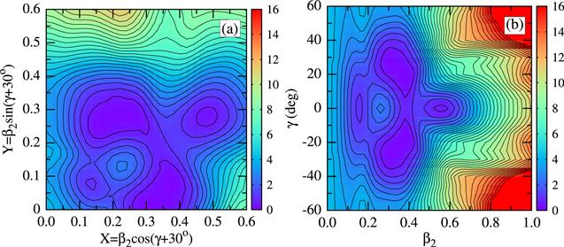
Figure 1. Projections of calculated total energy on the (X, Y) (a) and (β2, γ) (b) planes for ${}_{92}^{230}$U138. The energy interval between neighboring contour lines is 0.5 MeV. See the text for more details. |
Figure 2 illustrates the potential energies projected on the (β2, γ) planes with the consideration of different hexadecapole deformation degrees of freedom. For instance, in figures 2(a)–(d), the energy minimization is respectively performed over α40, α42, α44 and β4 at each deformation grid (β2, γ). One can see that the α40 deformation may result in a large decrease in energy. Calculations show the occurrence of non-zero triaxial minima after considering α42 and α44 deformations, as seen in figures 2(b) and (c). Not only the positions but also the shapes of the potential-energy surface near the minima are different, indicating the different effects on nuclear structure. To synthetically consider the different hexadecapole deformation degrees of freedom, we show the map of minimized energy over β4, according to the relationship e.g. in equation (5 ). However, the present results show that the different local minima may coexist depending on the selected deformation space. In fact, the full space expanded by the spherical harmonics, as seen in equation (4 ), is infinite in principle. The complexity of the nuclear shape is similar (or even equivalent) to the nuclear interaction. Reasonable selection of the deformation subspace in different mass regions and/or different spin and excitation conditions is worth exploring depending on experiences.
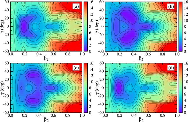
Figure 2. Similar to figure 1(b) but the energy minimization was respectively performed over the hexadecapole deformation degrees of freedom α40, α42, α44 and β4 in (a), (b), (c) and (d); and the energy minimum (in MeV) and equilibrium deformations (${E}_{\min };$ β2, γ, α4μ=0,2,4 or β4) are respectively (−5.2731; 0.20, 0°, −0.03), (−2.3548; 0.26, 30°, 0.01), (−2.9026; 0.32, 30°, 0.06) and (−5.2421; 0.20, 0°, −0.03). The energy interval between two contour lines is 1 MeV. |
In order to understand how dependent the calculated total energies are on these hexadecapole deformations α4μ=0,2,4 , figure 3 illustrates the corresponding 2D maps for ${}_{92}^{230}$U138 projected on the (β2, α4μ=0,2,4) and (β2, β4) planes (we focus on the even-μ components presently). To separately investigate the effects of different hexadecapole deformation parameters on the energy surfaces, in the left four subfigures of figure 3, we perform the calculations in 2D deformation spaces displayed by the horizontal and vertical coordinates, ignoring other degrees of freedom. It needs to be stressed that the hexadecapole deformation β4 involves the fixed relationships of {α4μ=0,2,4} and γ, as mentioned above. For instance, three deformation parameters {α4μ=0,2,4} can be determined in terms of a pair of given β2 and γ values. It can be seen from the left panel of figure 3 that the α40 (equivalently β4 at γ = 0°) deformation plays an important role in changing the energy minima, similar to the case in figure 2. The deformation spaces including the non-axial deformation parameters α42 and α44 can generate three energy minima but the energies are higher than that in the (β2, α40) plane. In the right part, at each deformation point of the corresponding map, the minimization is performed over triaxial deformation γ. Indeed, one can find that non-zero {α4μ=0,2,4} values appear at the minimum position, indicating that the three {α4μ=0,2,4} deformations play a role during the calculations; see e.g. figures 3(e)–(g). For simplicity of calculation and simultaneously including the effects of three such hexadecapole deformation parameters, the total energy projection on the (β2, β4) plane is illustrated in figure 3(h), minimized over γ. In the following investigation, the hexadecapole deformation β4 parameter is selected, which can give the collective coordinates {α4μ=0,2,4} by combining the γ parameter. Similar to the γ deformation, the β4 deformation has an obvious influence on the energy minimum for this nucleus, resulting in a strong energy reduction at the first minimum.
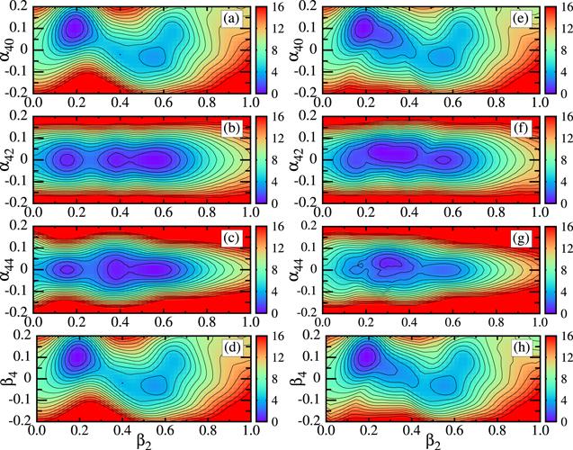
Figure 3. Similar to figure 2 but projections on the (β2,α40), (β2,α42), (β2,α44) and (β2,β4) planes for ${}_{92}^{230}$U138. In the (a), (b), (c) and (d) subplots, the triaxial deformation γ was set to zero during the calculations and the energy minimum (in MeV) and equilibrium deformations (${E}_{\min };$ β2, α4μ=0,2,4 or β4) are respectively (−5.2041; 0.20, 0.10), (−1.5279; 0.56, 0.00), (−1.5279; 0.56, 0.00) and (−5.2041; 0.20, 0.10). In the right four subfigures (e), (f), (g) and (h), the minimization was performed over γ at each mesh grid and, similarly, the values (${E}_{\min };$ β2, γ, α4μ=0,2,4 or β4) are respectively (−5.2041; 0.20, 0°, 0.10), (−2.3059; 0.26, 34°, 0.04), (−3.5264; 0.28, 32°, 0.02) and (−5.2041; 0.20, 0°, 0.10). |
In figure 4, we provide further evolution information on the total energy and its different components in functions of the quadrupole deformation β2 for ${}_{92}^{230}$U138, primarily aiming to show the impact of triaxial γ and hexadecapole β4 deformations on these energies. In the left panel, subfigures (a)–(d) represent the total energy, together with the macroscopic LD energy Eld, shell correction δEshell and pairing correlation δEpair, in functions of β2 at three selected γ values. For simplicity, other deformation degrees of freedom are ignored. One can see that the macroscopic LD energies slightly increase with increasing triaxial deformation γ at relatively large β2 deformation (e.g. after β2 = 0.6). For β2 < 0.4, the changed γ deformations have almost nothing to do with the LD energies. The shell corrections exhibit a large staggering both with changing β2 and γ, leading to similar trends in the corresponding total energies. The differences in total energies at the three γ values are mainly from shell corrections; see e.g. figure 4(c). Both the LD energy and pairing correlation have small effects with changing β2 and γ. Similarly, in the right part, e.g. from figure 4(e) to figure 4(h), the results are illustrated at three selected β4 deformation values. The β4 deformation mainly affects the microscopic shell effect. For the macroscopic energies, it seems that a critical point β2 ≃ 0.55 exists. Before (after) this point, the LD energies increase (decrease) with increasing β4. In addition, it can be noticed (cf table 1) that the inclusion of the β4 deformation is critical to reproducing the experimental β2 value and/or other theoretical results.
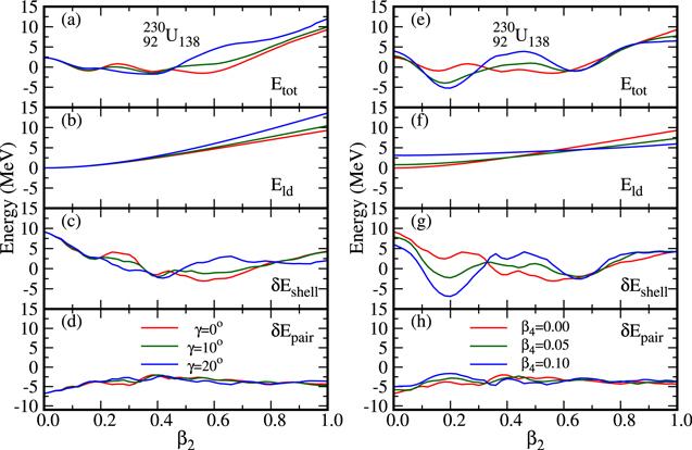
Figure 4. Left: Calculated total-energy Etot (a) curves against the quadrupole deformation β2 at three cases γ = 0°,10° and 20°, together with its macroscopic component Eld (b), microscopic shell correction δEshell (c) and pairing-energy contribution δEpair (d), for the nucleus ${}_{92}^{230}$U138. Other deformation parameters are ignored. Right: Similar to the left but with the corresponding three energy curves respectively plotted at β4 = 0.00, 0.05 and 0.10. |
Table 1. Calculated results (PES) for ground-state equilibrium deformation parameters β2 and β4 for even–even 226−230Th,228−232U and 230−234Pu, together with the FY+FRDM(FF) [62], HFBCS [63], and ETFSI [64] calculations and partial experimental (Exp.) β2 values [59] for comparison. |
| Nuclei | β2 | β4 | |||||||
|---|---|---|---|---|---|---|---|---|---|
| PESa | FF | HFBCS | ETFSI | Exp.b | PES | FF | HFBCS | ETFSI | |
| ${}_{90}^{226}$Th136 | 0.160 | 0.173 | 0.20 | 0.17 | 0.230 | 0.096 | 0.111 | 0.04 | 0.08 |
| ${}_{90}^{228}$Th138 | 0.174 | 0.182 | 0.21 | 0.19 | 0.230 | 0.098 | 0.112 | 0.04 | 0.08 |
| ${}_{90}^{230}$Th140 | 0.185 | 0.198 | 0.21 | 0.19 | 0.246 | 0.099 | 0.115 | 0.04 | 0.08 |
| ${}_{92}^{228}$U136 | 0.177 | 0.191 | 0.21 | 0.19 | — | 0.103 | 0.114 | 0.04 | 0.09 |
| ${}_{92}^{230}$U138 | 0.191 | 0.199 | 0.21 | 0.19 | 0.260 | 0.105 | 0.115 | 0.04 | 0.09 |
| ${}_{92}^{232}$U140 | 0.200 | 0.207 | 0.22 | 0.21 | 0.264 | 0.102 | 0.117 | 0.03 | 0.08 |
| ${}_{94}^{230}$Pu136 | 0.189 | 0.198 | 0.25 | 0.19 | — | 0.098 | 0.115 | 0.03 | 0.09 |
| ${}_{94}^{232}$Pu138 | 0.200 | 0.208 | 0.25 | 0.21 | — | 0.098 | 0.117 | 0.03 | 0.08 |
| ${}_{94}^{234}$Pu140 | 0.208 | 0.216 | 0.25 | 0.22 | — | 0.094 | 0.109 | 0.03 | 0.07 |
The calculated ground-state ∣γ∣ values of these nuclei are less than 2◦. | |
The uncertainties for deduced β2 values are no more than 0.011; see [59] for details. |
In the pairing-energy calculation, both the pairing model and the pairing strength are critical and controversial. A detailed discussion of these aspects is beyond the scope of the present work (we refer the interested readers to e.g. [57]). Here, in figure 5, we illustrate the impacts of the adjustments to the pairing strength on pairing contributions and total energies. As mentioned in [60], for the selected pairing model, the pairing strength G (≡FG0) can be adjusted by comparing the theoretical pairing gap with experimental data. It seems from figure 5 that the pairing strength continuously affects the pairing correlation, translating the energy curves. The negative δEpair originates from short-range attractions of paired nucleons (as expected, the larger the factor F is, the stronger the attraction).
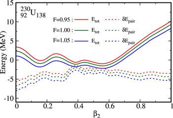
Figure 5. Total energy and pairing correlation curves against the quadrupole deformation β2 at the pairing-strength factor F = 0.95, 1.00 and 1.05 for ${}_{92}^{230}$U138. |
In functions of β2 and β4, figure 6 illustrates the calculated proton and neutron single-particle levels (near the Fermi levels) which correspond to the eigenstates of the one-body WS Hamiltonian. Usually, a set of conserved quantum numbers (associated with a complete set of commuting observables) are used for labeling the corresponding single-particle levels and wave functions. In the spherical case, for instance, the quantum numbers n, l and j, corresponding to the principal quantum number, the orbital angular momentum, and the total angular momentum, respectively, are adopted. Similar to atomic spectroscopy, the notations s, p, d, f, g, h ⋯ are used for l = 0, 1, 2, 3, 4, 5 ⋯, respectively. Due to the strong spin–orbit coupling, the single particle level with l splits into two levels with j = l ± 1/2, which has 2j + 1 degenerate states. From figure 6, one can see that the spherical shell gaps, e.g. Z = 82 and N = 126, are reproduced at β2 = 0.0. Once the deformed shape occurs, the 2j + 1 degeneracy is broken and the level labeled by nlj splits into j + 1/2 components. Each component (level) is typically double degenerate, due to Kramers degeneracy. The asymptotic Nilsson quantum numbers Ωπ[NnzΛ] are often used for describing the deformed single-particle level. Here, note that N is the total oscillator shell quantum number; nz stands for the number of oscillator quanta in the z direction (the direction of the symmetry axis); Λ is the projection of angular momentum along the symmetry axis; Σ is the projection of intrinsic spin along the symmetry axis; Ω is the projection of total angular momentum j (including orbital l and spin s) on the symmetry axis; and Ω = Λ + Σ. It should be pointed out that the virtual crossing removal [61] of single-particle levels with the same symmetries in these plots is not performed but this does not affect the identification of the single-particle levels. From this figure, it can be found that the β4 deformation plays a critical role during the shell evolution. For example, the shell gap does not appear at β2 ≈ 0.20 near the Fermi surface for either protons or neutrons. However, the energy gaps clearly appear at e.g. β4 ≈ 0.10, in good agreement with the following calculations (e.g. cf table 1).

Figure 6. Calculated neutron (top) and proton (bottom) single-particle energies as functions of the quadrupole deformation β2 (left) and hexadecapole deformation β4 for ${}_{92}^{230}$U138, focusing on the domain near the Fermi surface. The levels with positive and negative parities are respectively denoted by red solid and blue dotted lines. Spherical single-particle orbitals (i.e., at β2 = 0.0) in the window of interest are labeled by the quantum numbers nlj. |
Table 1 illustrates the calculated quadrupole deformation β2 and hexadecapole deformation β4 for nine even–even nuclei on the selected β4 deformation island, together with the available experimental data [59] and/or other accepted theories for comparison. As seen in this table, other theoretical calculations include the results given by the fold-Yukawa (FY) single-particle potential and the finite-range droplet model (FRDM) [62], the Hartree–Fock-BCS (HFBCS) [63] and the extended Thomas−Fermi plus Strutinsky integral (ETFSI) methods [64]. One can find that all the theoretical results underestimate the data. These theoretical values are somewhat model-dependent but in basic agreement with each other. Relatively, the HFBCS calculation gives the largest β2 but the smallest β4 values. Our calculated β2 deformations are slightly smaller than the FF and ETFSI calculations. As discussed by Dudek et al [65], the underestimated quadrupole deformation β2 should be slightly modified by the empirical relationship 1.10β2-$0.03{\left({\beta }_{2}\right)}^{3}$ in the WS-type mean-field calculations. Nevertheless, the β4 values lie between the FF and ETFSI calculations. It should be noted that the dynamical effects (e.g. the vibrating coupling) may to some extent be responsible for the underestimations of β2 values (the data extracted from BE(2) automatically include the vibrating effect, e.g. see [58] and references therein), especially in the soft nuclei.
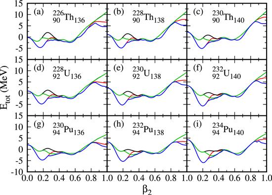
To exhibit the depth and softness properties of the minimum near the equilibrium shape, we show four types of total energy curves in functions of β2 for nine selected nuclei 226,228,230Th, 228,230,232U and 230,232,234Pu in figure 7. Note that the blue, red, green, and black lines respectively correspond to those curves whose energies are minimized over γ and β4; β4; γ; and none. One can notice that the nuclear shapes are very soft and several coexisting shapes may be produced if just considering the triaxial deformation degree of freedom. The inclusion of the triaxial γ deformation leads to the disappearance of the barrier between β2 ∼ 0.2 and 0.3, even producing an energy pocket (e.g. see the green lines in 232U and 232,234Pu). In addition, it seems that the hexadecapole deformation β4 plays a critical role in reproducing the comparable values with data and/or previous theories. The minima e.g. between β2 = 0.1 and 0.2 are reduced by 4−5 MeV and, simultaneously, the equilibrium β2 deformations of the minima increase owing to the β4 effects. In the large deformed region (e.g. β > 0.8), both the β4 and β4-induced γ deformations (without β4, the γ deformation does not work, e.g. see the overlapped green and black lines) decrease the outer barriers. In previous studies [33, 66], it was pointed out that the triaxial γ and octupole deformation β3 could reduce the outer barriers. To explore a more reasonable deformation subspace, especially near the outer barrier, it may be necessary to simultaneously consider, at least, the triaxial, octupole, and hexadecapole correlations.
Figure 7. Four types of deformation energy curves as the function of quadrupole axial deformation β2 for nine nuclei 226,228,230Th, 228,230,232U and 230,232,234Pu. The lines with different colors denote whether or not the total energy at each β2 was minimized and, if so, with respect to what deformation parameter(s). For instance, at each β2 point of the green line, the minimization was performed over γ (blue, over γ and β4; red, over β4; and black, over none). Note that the black and blue curves always occupy the highest and lowest positions, respectively, though they may be not displayed fully due to the strong overlap with other ones. |
4. Summary
In summary, we have investigated the effects of the axial and nonaxial quadrupole and hexadecapole deformations on potential energy surfaces of nuclei on the β4 island (around 230U) within macroscopic−microscopic frameworks. The calculations are performed in multidimensional (β2, γ, β4) and (β2, γ, α4μ) deformation spaces. It is found that the hexadecapole deformations strongly modify the nuclear potential landscapes in these nuclei. Near the equilibrium energy pocket, the hexadecapole deformation β4 can decrease the minimum by 4–5 MeV. In the large deformed region, the β4 deformation has an important influence on the outer barrier and, even during the evolution process from the first minimum to the strongly elongated β2 region, still plays a certain role. The hexadecapole deformations are critical degrees of freedom in research on the nuclear equilibrium shape and fission process. Both experimentally and theoretically, it is to an extent meaningful to further study the hexadecapole deformations in nuclei.