


1. Introduction
Modern cosmology has plunged into a data-driven era. According to various accumulated observational evidence [1–9], the Universe is under an accelerated expansion which gives rise to the concept of dark energy (DE). It has been observed that the Universe contains 70% dark energy components and the remaining 30% includes baryons and cold dark matter. In the context of general relativity, a very simple candidate for this DE is the cosmological constant Λ, known as the Λ-cold-dark-matter (ΛCDM) model which is verified by recent highly precise Planck cosmic microwave background measurements [10]. However, it mainly suffers from two problems, the cosmological constant problem and the cosmic coincidence problem [11]. As we know very little about the realistic nature of DE, many cosmologists have proposed either modified theories or dynamical DE models to resolve these problems.
The holographic dark energy (HDE) is a dynamical DE model and the holographic principle (HP) is the foundation of this model [12, 13]. Being a proposal of quantum gravity, the HP states that the entropy of any system is not related to its volume but to its surface area. According to the principle, the maximum entropy limit set by the system should not be greater than the entropy of a black hole of the same size. This gives a connection between the short distance (ultra-violet) cut-off and long distance (infra-red) cut-off. Mathematically, in accordance with the HP, for a system with size L and an ultra-violet (UV) cut-off Λ, the vacuum energy density ρh should relate to the boundary surface of a system in a way ${\rho }_{h}\leqslant {{M}_{P}}^{2}{L}^{-2}$. The energy density of HDE at the saturation of the system is given as ${\rho }_{h}=3{b}^{2}{{M}_{P}}^{2}{L}^{-2}$ where b is a numerical constant and MP denotes the reduced Planck constant. The HDE energy density depends on the choice of infra-red(IR) cut-off which represents the large length scale of the Universe. Hsu [14] considered the Hubble horizon as an IR cut-off and found that the HDE model could not drive the observable late-time expansion of the Universe. In a paper, Li [15] found that assuming the event horizon as an IR cut-off could drive the accelerated expansion of the Universe but it faced the causality problem. Some other HDE models with different IR cut-offs have been proposed in the literature, e.g., agegraphic dark energy [16, 17], Ricci scale dark energy [18]. Granda and Oliveros [19] came up with a new IR cut-off which is a combination of the Hubble parameter and its time derivative to solve the causality problem. This cut-off has been studied by many authors [20–33] to explain the present-day evolution of the Universe.
The imperfect fluids including shear and bulk viscosity play a key role in the dynamics of the Universe. The viscous term arises when the fluid expands (or contracts) rapidly and ceases to be in thermodynamic equilibrium. It is a measure of pressure required to restore the thermodynamic equilibrium. Eckart [34] proposed the general theory for the relativistic imperfect fluid by considering the first-order deviation from equilibrium. Later on, this theory was modified by Landau and Lifshitz [35]. This theory suffers some problems in its formulation, e.g., equilibrium states are unstable and non-causal [36]. In fact, the neglected second-order terms are responsible for this problem. In order to remove such a problem, a second-order theory in a relativistic framework was developed by Israel and Stewart [37], which was stable and causal. However, the Eckart theory can be recovered from Israel-Stewart (IS) theory when the relaxation time becomes zero. Therefore, in the limit of vanishing relaxation time, the Eckart theory is a good approximation to IS theory. Due to the simple form of Eckart's theory and considering that the relaxation time goes to zero in the late-time evolution of the Universe, it has been studied by many authors to observe the effect of bulk viscous fluid in the late-time evolution of the Universe.
In the case of a homogenous and isotropic Universe, assuming the cosmological principle, the dissipative process within a thermodynamical approach can be modeled as a bulk viscosity. The bulk viscous pressure is characterized by the bulk viscous coefficient ξ. There is various parametrization of ξ available in the literature. The simplest parametrization of the bulk viscous coefficient is considered to be constant, i.e., ξ = ξ0. The other parametrization has been considered as ξ = ξ1H, where ξ1 is a constant and H is the Hubble parameter, and a linear combination form ξ = ξ0 + ξ1H. In recent years, many authors [38–61] have discussed viscous cosmology to show the late-time evolution of the Universe by assuming these parameterized forms of the bulk viscous coefficient. Some authors [62–66] have studied the viscous cosmological model with bulk viscous coefficient depending on both expansion and acceleration rates, i.e., $\xi ={\xi }_{0}\,+{\xi }_{1}H+{\xi }_{2}\ddot{a}/\dot{a}$, where ξ2 is a constant, a denotes the scale factor, and the dot represents the differentiation with respect to cosmic time.
It has already been discovered that a non-viscous HDE model with a Granda–Oliveros IR cut-off does not show the observable evolution of the Universe [60]. In this paper, we examine the viscous effect in a dynamical HDE model with the new IR cut-off suggested by Granda and Oliveros [19] to achieve the present day evolution of the Universe. In this dynamical HDE model, we consider that our Universe is filled with dark matter consisting of bulk viscosity and HDE. We study the evolution of the Universe by considering a more generalized form of bulk viscous coefficient as proposed in the papers [62, 63]. We constrain the model to get the best-fit values of model parameters by using different observational data such as Type Ia supernova (Pantheon), Hubble data, strong lensing data, and the local Hubble value of SH0ES. We distinguish the viscous model from the standard ΛCDM model by studying the statefinder parameters and cosmographic parameters.
This paper is divided into the following sections: section 2 presents the basic equations of the HDE model with bulk viscosity and the solutions for the Hubble parameter, along with some other main cosmological parameters. In section 3 , we estimate the best-fit values of parameters using the latest observational data. We use the best-fit values to discuss the evolution of the different cosmological parameters in section 4 . A discussion on statefinder parameters and cosmographic parameters is presented in section 5 . The conclusion is in the last section 6 .
2. Bulk viscous HDE model
For presenting the bulk viscous HDE, we start from an isotropic and homogeneous flat Friedmann–Lemaitre–Robertson–Walker (FLRW) metric which is defined by the line element
$\begin{eqnarray}{{\rm{d}}{s}}^{2}=-{{\rm{d}}{t}}^{2}+{a}^{2}(t)\left[{{\rm{d}}{r}}^{2}+{r}^{2}{\rm{d}}{{\rm{\Omega }}}^{2}\right],\end{eqnarray}$
where ${\rm{d}}{{\rm{\Omega }}}^{2}={\rm{d}}{\theta }^{2}+{\sin }^{2}\theta {\rm{d}}{\phi }^{2}$ and a(t) is the scale factor of the Universe. Throughout we use units 8πG = c = 1.It has been observed that the HDE model with Granda–Oliveros as the IR cut-off does not show the phase transition [60]. However, the observations indicate a transition phase from deceleration to acceleration during the evolution of the Universe. The recent works on bulk viscosity [62–66] show that this dissipative fluid plays an important role in describing the late-time evolution. Therefore, it will be worthy to discuss the HDE model with bulk viscosity by using the Granda–Oliveros IR cut-off to explain phase transition.
In a homogeneous and isotropic Universe, the only dissipative process allowed is the bulk viscosity. It is well known that bulk viscosity plays an important role in the Universe dynamics at the background level because it satisfies the cosmological principle. The viscous process fundamentally changes the equation of motion of relativistic fluids through the addition of new terms of hydrodynamics in energy-momentum tensor.
Hence, in dissipative cosmology with bulk viscosity, Einstein's field equations modify to ${R}_{\mu \nu }-\tfrac{1}{2}{g}_{\mu \nu }R={T}_{\mu \nu }^{\mathrm{eff}}$, where ${T}_{\mu \nu }^{\mathrm{eff}}$ is the effective energy-momentum tensor of the cosmic fluids including the bulk viscosity. This tensor is considered as ${T}_{\mu \nu }^{\mathrm{eff}}=(\rho +P){u}_{\mu }{u}_{\nu }+{{Pg}}_{\mu \nu }$, where ρ = ρm +ρh is the total energy density of matter and HDE, and P is the effective fluid pressure which may be defined as P = pm + Π + ph. Here pm, Π and ph represent the dark matter pressure, bulk viscous pressure and HDE pressure, respectively.
The first approach to studying the relativistic bulk viscosity process in thermodynamics systems is based on the Eckart theory [32]. It is known that this theory is unstable and non-causal against perturbations around the thermodynamical equilibrium state [36], i.e., it describes that all the equilibrium states are unstable and the signals can propagate through the fluids faster than the speed of light, i.e., with superluminal velocities. These problems could be traced back to their restriction to first-order deviations from equilibrium. In order to solve these problems, Israel and Stewart [37] proposed a second-order full causal theory in a relativistic framework. Despite instability and non-causality, Eckart's theory is still suitable for cosmological investigations while dealing with the accelerating Universe with bulk viscous fluids. This is due to the fact that this theory is a good approximation to the IS theory in the limit when the relaxation time vanishes in the late time. Another reason is that Eckart's theory is less complicated than the IS theory, so by taking advantage of the equivalence of both theories at this limit, it has been widely used by many authors to characterize the bulk viscous fluid in describing the late-time acceleration when the relaxation time goes to zero.
In Eckart formalism [34], the viscous pressure Π is considered as ${\rm{\Pi }}=-\xi {u}_{;a}^{a}=-3\xi H$, where ξ is the bulk viscous coefficient, ua is the four-velocity vector and H is the Hubble parameter. The bulk viscous coefficient ξ is conventionally chosen to be a positive quantity on thermodynamical grounds.
Let us consider the FLRW Universe (1 ) dominated by pressureless dark matter with the viscous term and the energy of the HDE. The non-vanishing equations of Einstein's field equations are
$\begin{eqnarray}3{H}^{2}={\rho }_{m}+{\rho }_{h}\end{eqnarray}$
and $\begin{eqnarray}(\dot{{\rho }_{m}}+\dot{{\rho }_{h}})+3({\rho }_{m}+{\rho }_{h}+{p}_{h}-3\xi H)H=0,\end{eqnarray}$
where an overdot denotes the derivative with respect to cosmic time t and $H=\dot{a}/a$ is the Hubble parameter.Assuming that there is no interaction between the dark matter with bulk viscosity and HDE, the conservation equation (3 ), therefore, conserves separately, which is given by
$\begin{eqnarray}{\dot{\rho }}_{m}+3H({\rho }_{m}-3H\xi )=0\end{eqnarray}$
and $\begin{eqnarray}{\dot{\rho }}_{h}+3H(1+{\omega }_{h}){\rho }_{h}=0,\end{eqnarray}$
where ph = ωhρh is the equation of state for HDE. Here, ωh is the equation of state (EoS) parameter for HDE.In the HDE model, as discussed in section 1 , the UV cut-off is related to the vacuum energy, and the IR cut-off is related to the large scale of the Universe, for example, the Hubble horizon, future event horizon or particle horizon. Taking L as the size of the current Universe, for instance, using the Hubble scale, the resulting energy density is comparable to the present-day DE. Hsu [14] studied the HDE model with the Hubble horizon as the IR cut-off and found that the evolution of DE is the same as that of the dark matter (dust matter). Therefore, it cannot drive the Universe to accelerated expansion. The same appears if one chooses the particle horizon of the Universe as the length scale L. However, Li [15] studied the HDE model with the event horizon as the IR cut-off and found that the holographic DE not only gives the observation value of DE in the Universe but also can drive the Universe to an accelerated expansion phase. In that case, however, an obvious drawback concerning causality appears in this proposal. An event horizon is a global concept of spacetime and the existence of the event horizon of the Universe depends on the future evolution of the Universe. Therefore, the event horizon exists only for a Universe with forever accelerated expansion. Granda–Oliveros [19] proposed a new IR cut-off for HDE, which is a combination of the Hubble parameter and its time derivative. This model depends on local quantities and avoids the problem of causality which appears using the event horizon area as the IR cut-off.
The new IR cut-off for HDE as proposed by Granda and Oliveros [19] is given by
$\begin{eqnarray}{\rho }_{h}=3(\alpha {H}^{2}+\beta \dot{H}),\end{eqnarray}$
where α and β are the dimensionless parameters to be computed by the current observational data.Granda and Oliveros [19] argued that since the underlying origin of the holographic DE is still unknown, the inclusion of the time derivative of the Hubble parameter may be expected as this term appears in the curvature scalar, and has the correct dimension. This kind of density may appear as the simplest case of more general $f(H,\dot{H})$ holographic density in the FLRW background. Comparing (6 ) with the HDE density ${\rho }_{h}=3{b}^{2}{M}_{P}^{2}{L}^{-2}$ shows that the corresponding IR cut-off for model (6 ) is2 ), (4 ) and (5 ) give the evolution equation for the Hubble function as
$\begin{eqnarray}L={H}^{-1}{\left(1+\displaystyle \frac{\beta }{\alpha }\displaystyle \frac{\dot{H}}{{H}^{2}}\right)}^{-1/2}\end{eqnarray}$
which depends on local quantities and avoids the causality problem. Using the above-mentioned energy density for HDE, equations ( $\begin{eqnarray}\dot{H}+\displaystyle \frac{3(1+\alpha {\omega }_{h})}{(2+3\beta {\omega }_{h})}{H}^{2}=\displaystyle \frac{3\xi H}{2+3\beta {\omega }_{h}}.\end{eqnarray}$
Using $x=\mathrm{ln}a$, the above equation can be transformed into $\begin{eqnarray}h^{\prime} +\displaystyle \frac{3(1+\alpha {\omega }_{h})}{(2+3\beta {\omega }_{h})}h=\displaystyle \frac{3\xi }{(2+3\beta {\omega }_{h}){H}_{0}},\end{eqnarray}$
where h = H/H0 is the dimensionless Hubble parameter and $h^{\prime} ={dh}/{dx}$ i.e. the prime indicates the derivative with respect to $\mathrm{ln}a$. The above evolution equation can analytically be solved provided to assume a specific form of bulk viscous coefficient ξ.In an expanding Universe, the bulk viscous coefficient may depend on both the velocity and acceleration. The most logical form can be a linear combination of three terms: the first term is a constant ζ0, the second term is proportional to the Hubble parameter, which characterizes the dependence of the bulk viscosity on velocity, and the third is proportional to $\ddot{a}/\dot{a}$, characterizing the effect of acceleration on the bulk viscosity. Thus, we consider the parameterized bulk viscous coefficient as a combination of three terms which is given by [63]11 ) reduces to12 ) into (9 ), we finally get the evolution equation as15 ) gives the solution of scale factor which has power-law form in early times and an exponential expansion in the late-time evolution of the Universe. Therefore, we obtain a solution that shows a phase transition from deceleration epoch to acceleration epoch during the evolution. The transition from decelerated to accelerated phase can be further explained by defining the deceleration parameter q as $q=-\tfrac{a\ddot{a}}{{\dot{a}}^{2}}=-1-\tfrac{a}{h}\tfrac{{\rm{d}}{h}}{{\rm{d}}{a}}$. Thus, from equation (14 ), we get16 ), the present value of q(z) corresponds to z = 0 is
$\begin{eqnarray}\xi ={\xi }_{0}+{\xi }_{1}\displaystyle \frac{\dot{a}}{a}+{\xi }_{2}\displaystyle \frac{\mathop{ä}}{\dot{a}}.\end{eqnarray}$
In terms of the Hubble parameter, this can be written as $\begin{eqnarray}\xi ={\xi }_{0}+{\xi }_{1}H+{\xi }_{2}\left(\displaystyle \frac{\dot{H}}{H}+H\right),\end{eqnarray}$
where ξ0, ξ1 and ξ2 are constants. Defining the dimensionless bulk viscous parameters ζ0 = ξ0/H0, ζ1 = ξ1 + ξ2, ζ2 = ξ2 and ζ = ξ/H0, equation ( $\begin{eqnarray}\zeta ={\zeta }_{0}+{\zeta }_{1}h+{\zeta }_{2}h^{\prime} .\end{eqnarray}$
Using ( $\begin{eqnarray}h^{\prime} +\displaystyle \frac{3(1+\alpha {\omega }_{h}-{\zeta }_{1})}{(2+3\beta {\omega }_{h}-3{\zeta }_{2})}h=\displaystyle \frac{3{\zeta }_{0}}{2+3\beta {\omega }_{h}-3{\zeta }_{2}}.\end{eqnarray}$
Integrating the above equation to get the solution of the dimensionless Hubble parameter as $\begin{eqnarray}\begin{array}{l}h=\displaystyle \frac{{\zeta }_{0}}{1+\alpha {\omega }_{h}-{\zeta }_{1}}+\left(1-\displaystyle \frac{{\zeta }_{0}}{1+\alpha {\omega }_{h}-{\zeta }_{1}}\right)\\ \quad \times \,{a}^{-\tfrac{3(1+\alpha {\omega }_{h}-{\zeta }_{1})}{(2+3\beta {\omega }_{h}-3{\zeta }_{2})}},\end{array}\end{eqnarray}$
which can further be simplified by considering a normalized relationship between the scale factor and redshift, a = (1 + z)−1 to get the solution for the Hubble parameter as $\begin{eqnarray}\begin{array}{l}H={H}_{0}\left[\displaystyle \frac{{\zeta }_{0}}{1+\alpha {\omega }_{h}-{\zeta }_{1}}+\left(1-\displaystyle \frac{{\zeta }_{0}}{1+\alpha {\omega }_{h}-{\zeta }_{1}}\right)\right.\\ \quad \left.\times {(1+z)}^{\tfrac{3(1+\alpha {\omega }_{h}-{\zeta }_{1})}{(2+3\beta {\omega }_{h}-3{\zeta }_{2})}}\right].\end{array}\end{eqnarray}$
It should be noted that for ζ0, ζ1 and ζ2 equal to zero, the Hubble parameter gives $H={H}_{0}{(1+z)}^{3(1+\alpha {\omega }_{h})/(2+3\beta {\omega }_{h})}$, which corresponds to the power-law solution of the HDE Universe. Further, α = 0 and β = 0 reduce the model to the matter-dominated Universe H = H0(1 + z)3/2, whose solution gives the power-law expansion of the Universe. However, equation ( $\begin{eqnarray}\begin{array}{l}q=-1+\displaystyle \frac{3(1+\alpha {\omega }_{h}-{\zeta }_{1})}{2+3\beta {\omega }_{h}-3{\zeta }_{2}}\\ \quad \times \displaystyle \frac{\left(1-\tfrac{{\zeta }_{0}}{1+\alpha {\omega }_{h}-{\zeta }_{1}}\right){\left(1+z\right)}^{\tfrac{3(1+\alpha {\omega }_{h}-{\zeta }_{1})}{2+3\beta {\omega }_{h}-3{\zeta }_{2}}}}{\left[\tfrac{{\zeta }_{0}}{1+\alpha {\omega }_{h}-{\zeta }_{1}}+\left(1-\tfrac{{\zeta }_{0}}{1+\alpha {\omega }_{h}-{\zeta }_{1}}\right)\,{\left(1+z\right)}^{\tfrac{3(1+\alpha {\omega }_{h}-{\zeta }_{1})}{(2+3\beta {\omega }_{h}-3{\zeta }_{2})}}\right]}\end{array}\end{eqnarray}$
which depends on cosmic time and hence shows the phase transition. We observe that q(z) approaches to −1 in the late time (negative redshift). The transition redshift ${z}_{\mathrm{tr}}$ can be obtained by substituting q = 0 in the above equation, which is obtained as $\begin{eqnarray}\begin{array}{l}{z}_{\mathrm{tr}}=-1\\ +\,{\left[1+\displaystyle \frac{(1+\alpha {\omega }_{h}-{\zeta }_{1})(1+3(\alpha -\beta ){\omega }_{h}-3({\zeta }_{0}+{\zeta }_{1}-{\zeta }_{2}))}{{\zeta }_{0}(2+3\beta {\omega }_{h}-3{\zeta }_{2})}\right]}^{-\tfrac{2+3\beta {\omega }_{h}-3{\zeta }_{2}}{3(1+\alpha {\omega }_{h}-{\zeta }_{1})}}.\end{array}\end{eqnarray}$
From ( $\begin{eqnarray}{q}_{0}=-1+\displaystyle \frac{3(1+\alpha {\omega }_{h}-{\zeta }_{1}-{\zeta }_{0})}{2+3\beta {\omega }_{h}-3{\zeta }_{2}}.\end{eqnarray}$
Let us derive one more parameter to discuss the evolution of the Universe. This parameter is known as the effective equation of state (EoS) parameter, which is defined as ${w}_{\mathrm{eff}}=-1-\tfrac{2a}{3h}\tfrac{{\rm{d}}{h}}{{\rm{d}}{a}}$. For this viscous HDE model we get $\begin{eqnarray}{w}_{\mathrm{eff}}=-1+\displaystyle \frac{2(1+\alpha {\omega }_{h}-{\zeta }_{1}-{\zeta }_{0})}{2+3\beta {\omega }_{h}-3{\zeta }_{2}}\displaystyle \frac{{\left(1+z\right)}^{\tfrac{3(1+\alpha {\omega }_{h}-{\zeta }_{1})}{2+3\beta {\omega }_{h}-3{\zeta }_{2}}}}{h}.\end{eqnarray}$
The present value of weff at z = 0 for our model is $\begin{eqnarray}{\omega }_{\mathrm{eff}}(z=0)=-1+\displaystyle \frac{2(1+\alpha {\omega }_{h}-{\zeta }_{1}-{\zeta }_{0})}{2+3\beta {\omega }_{h}-3{\zeta }_{2}}.\end{eqnarray}$
3. Data samples and methodology
In this section, following the derivation of H(z) obtained in (15 ), we constrain the space parameters (H0, ζ0, ζ1, ζ2, α, β, ωh) of viscous HDE model using the two different combinations of the following mentioned recent data sets.
3.1. Strong lensing system
In this paper, we use new data from the Strong Lensing System (SLS) to constrain the model parameters. Due to the presence of gravity, light rays that pass near matter are bent in accordance with the general theory of relativity, and this bending of light is strong enough to produce multiple images of the source. This phenomenon is known as strong gravitational lensing [67]. For elliptical galaxies acting as lenses, image separation depends on the mass of the lens and also on the angular diameter distance between the lens and the source, and also between the observer and the lens.
The chi-square function for 204 SLS in the redshift 0.063 < zl < 0.950 for the lens and 0.196 < zs < 3.595 for the source is given by [68]
$\begin{eqnarray}{\chi }_{\mathrm{SLS}}^{2}=\displaystyle \sum _{i=1}^{204}\displaystyle \frac{{[{D}^{\mathrm{th}}({z}_{{\rm{l}}},{z}_{{\rm{s}}},{\rm{\Theta }})-{D}^{\mathrm{obs}}({\theta }_{{\rm{e}}},{\sigma }^{2})]}^{2}}{{\left(\delta {D}^{\mathrm{obs}}\right)}^{2}},\end{eqnarray}$
where Θ is the free space parameter and Dobs = c2θe/4πσ2. The uncertainty of each Dobs measurement is calculated by $\begin{eqnarray}\delta {D}^{\mathrm{obs}}={D}^{\mathrm{obs}}\sqrt{{\left(\displaystyle \frac{\delta {\theta }_{{\rm{e}}}}{{\theta }_{{\rm{e}}}}\right)}^{2}+4{\left(\displaystyle \frac{\delta \sigma }{\sigma }\right)}^{2}},\end{eqnarray}$
where δθe and δσ are the error reported for the Einstein radius and velocity dispersion respectively.In the above equations, θe is the Einstein radius of the lens which is defined by a Singular Isothermal Sphere (SIS) as
$\begin{eqnarray}{\theta }_{{\rm{e}}}=4\pi \displaystyle \frac{{\sigma }_{\mathrm{SIS}}^{2}{D}_{{ls}}}{{c}^{2}{D}_{{\rm{s}}}},\end{eqnarray}$
where Dls is the angular diameter distances between the lens galaxy and the source and Ds is the angular diameter distances between the observer and the source, σSIS is the velocity dispersion of the lens galaxy and c is the speed of light.Now, Ds, in terms of redshift can be defined as21 ) is defined by the ratio Dth = Dls/Ds.
$\begin{eqnarray}{D}_{s}(z)=\displaystyle \frac{c}{(1+z)}{\int }_{0}^{{z}_{s}}\displaystyle \frac{{dz}^{\prime} }{H(z^{\prime} )}\end{eqnarray}$
and Dls is given by $\begin{eqnarray}{D}_{{ls}}(z)=\displaystyle \frac{c}{(1+z)}{\int }_{{z}_{l}}^{{z}_{s}}\displaystyle \frac{{dz}^{\prime} }{H(z^{\prime} )}.\end{eqnarray}$
Therefore, the theoretical distance Dth in equation (3.2. Hubble data
We use the updated collection of 57 Hubble H(z) data points between the redshift range 0.07 ≤ z ≤ 2.36 that consists of 31 points collected from the differential age (DA) technique and 26 data points received through line-of-sight BAO and other methods. The complete list of data is presented in table 1 with respective references, compiled by Sharov and Vasiliev [69]. The minimized chi-squared function for determining the best-fit values of the model is
$\begin{eqnarray}{\chi }_{{\rm{H}}({\rm{z}})}^{2}({\rm{\Theta }})=\displaystyle \sum _{i=1}^{57}\displaystyle \frac{{[H({z}_{i},{\rm{\Theta }})-{H}_{\mathrm{obs}}({z}_{i})]}^{2}}{{\sigma }_{{\rm{H}}({{\rm{z}}}_{i})}^{2}}\end{eqnarray}$
where H(zi, Θ) represents the theoretical values of the Hubble parameter with model parameters, Hobs(zi) is the observed values of the Hubble parameter and σi represents the standard deviation measurement uncertainty in Hobs(zi, Θ).Table 1. H(z) data in Km s−1 Mpc−1 consisting of 57 points (source: Sharov and Vasiliev, 2018). |
| DA Method (31 points) | |||||||
|---|---|---|---|---|---|---|---|
| z | H(z) | σh(z) | Ref. | z | H(z) | σh(z) | Ref. |
| 0.070 | 69 | 19.6 | [70] | 0.4783 | 80 | 99 | [74] |
| 0.90 | 69 | 12 | [71] | 0.480 | 97 | 62 | [70] |
| 0.120 | 68.6 | 26.2 | [70] | 0.593 | 104 | 13 | [72] |
| 0.170 | 83 | 8 | [71] | 0.6797 | 92 | 8 | [72] |
| 0.1791 | 75 | 4 | [72] | 0.7812 | 105 | 12 | [72] |
| 0.1993 | 75 | 5 | [72] | 0.8754 | 125 | 17 | [72] |
| 0.200 | 72.9 | 29.6 | [73] | 0.880 | 90 | 40 | [70] |
| 0.270 | 77 | 14 | [71] | 0.900 | 117 | 23 | [71] |
| 0.280 | 88.8 | 36.6 | [73] | 1.037 | 154 | 20 | [72] |
| 0.3519 | 83 | 14 | [72] | 1.300 | 168 | 17 | [71] |
| 0.3802 | 83 | 13.5 | [74] | 1.363 | 160 | 33.6 | [76] |
| 0.400 | 95 | 17 | [71] | 1.430 | 177 | 18 | [71] |
| 0.4004 | 77 | 10.2 | [74] | 1.530 | 140 | 14 | [71] |
| 0.4247 | 87.1 | 11.2 | [74] | 1.750 | 202 | 40 | [71] |
| 0.4497 | 92.8 | 12.9 | [74] | 1.965 | 186.5 | 50.4 | [76] |
| 0.470 | 89 | 34 | [75] | ||||
| BAO and other method (26 points) | |||||||
| z | H(z) | σh(z) | Ref. | z | H(z) | σh(z) | Ref. |
| 0.24 | 79.69 | 2.99 | [77] | 0.52 | 94.35 | 2.64 | [79] |
| 0.30 | 81.7 | 6.22 | [78] | 0.56 | 93.34 | 2.3 | [79] |
| 0.31 | 78.18 | 4.74 | [79] | 0.57 | 87.6 | 7.8 | [83] |
| 0.34 | 83.8 | 3.66 | [77] | 0.57 | 96.8 | 3.4 | [84] |
| 0.35 | 82.7 | 9.1 | [80] | 0.59 | 98.48 | 3.18 | [79] |
| 0.36 | 79.94 | 3.38 | [79] | 0.60 | 87.9 | 6.1 | [82] |
| 0.38 | 81.5 | 1.9 | [81] | 0.61 | 97.3 | 2.1 | [81] |
| 0.40 | 82.04 | 2.03 | [79] | 0.64 | 98.82 | 2.98 | [79] |
| 0.43 | 86.45 | 3.97 | [77] | 0.73 | 97.3 | 7.0 | [82] |
| 0.44 | 82.6 | 7.8 | [82] | 2.30 | 224 | 8.6 | [85] |
| 0.44 | 84.81 | 1.83 | [79] | 2.33 | 224 | 8 | [86] |
| 0.48 | 87.79 | 2.03 | [79] | 2.34 | 222 | 8.5 | [87] |
| 0.51 | 90.4 | 1.9 | [81] | 2.36 | 226 | 9.3 | [88] |
3.3. Type Ia supernovae (Pantheon data)
The confidence in Type Ia supernovae (SNe) as standard candles has been growing rapidly over the last two decades. The first strong indication of the accelerated expansion of the Universe was also given by the SNe observations. The latest compilation of Pantheon sample SNe has been used, which consists of 1048 data points from SNLS, SDSS, Pan-STARRS1, and a HST survey in the redshift range of 0.014 ≤ z ≤ 2.3 [89].
We can minimize the χ2 function for SNe as
$\begin{eqnarray}{\chi }_{\mathrm{SNe}}^{2}=\mu \,{C}^{-1}\,{\mu }^{{\rm{T}}},\end{eqnarray}$
where $\mu ={\mu }_{i}^{\mathrm{obs}}-{\mu }^{\mathrm{th}}$ and C is the covariance matrix of μobs given in [90]. The observed distance modulus is given in Ref.[91]. Also, the theoretical distance modulus is defined as $\begin{eqnarray}{\mu }^{\mathrm{th}}=5\,{{\rm{log}}}_{10}[{d}_{L}(z)/10{pc}]+{\text{}}M,\end{eqnarray}$
where M is the nuisance parameter and dL(z) is the dimensionless luminosity distance defined as [89] $\begin{eqnarray}{d}_{{\rm{L}}}(z)=(1+z)c{\int }_{0}^{z}\displaystyle \frac{{\rm{d}}{z}^{\prime} }{H(z^{\prime} ,{\rm{\Theta }})},\end{eqnarray}$
where Θ is the space parameters of the model and c is the speed of light.3.4. Local Hubble constant
In addition, we take the recently measured local Hubble constant H0 as H0 = 73.5 ± 1.4 km s−1Mpc−1 by SH0ES as mentioned in [92].
3.5. Methodology
We perform fitting to determine the best-fit values of model parameters using the Markov chain Monte Carlo (MCMC) method in the EMCEE library [93]. We consider two combinations of the latest datasets of SNe(Pantheon), H(z), SLS and local H0, namely, DS1: ${\chi }_{\mathrm{DS}1}^{2}={\chi }_{\mathrm{SNe}}^{2}+{\chi }_{{\rm{H}}({\rm{z}})}^{2}+{\chi }_{\mathrm{SLS}}^{2}+{\chi }_{{{\rm{H}}}_{0}}^{2}$ and DS2: ${\chi }_{\mathrm{DS}2}^{2}={\chi }_{\mathrm{SNe}}^{2}+{\chi }_{{\rm{H}}({\rm{z}})}^{2}+{\chi }_{\mathrm{SLS}}^{2}$. In our statistical analysis, we minimize the function χ2 for these data sets. The best-fit values of space parameters (Θ = H0, ζ0, ζ1, ζ2, α, ωh, β) of viscous HDE and (Θ = H0, ΩΛ, Ωm) of ΛCDM models obtained by both the combinations are provided in table 2. The likelihood contour at 1σ(68.3%) and 2σ(95.4)% confidence levels for both data sets is represented in figure 1. The data set DS1 fitted is shown by the red contours while the greyish contours are derived from the DS2 data set. In the following section, we present and discuss the results obtained from the above-mentioned data sets.
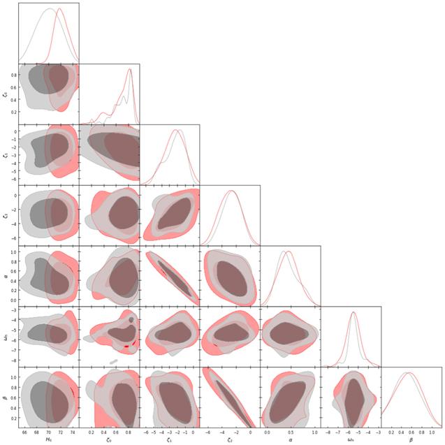
Figure 1. The likelihood contours at 68.3% CL and 95.4% CL for viscous HDE model correspond to DS1(red color) and DS2 (grey color) datasets. |
Table 2. The best-fit values of free parameters of HDE and ΛCDM models with errors from DS1 and DS2 datasets. |
| DS1 | DS2 | |||
|---|---|---|---|---|
| Model | HDE | ΛCDM | HDE | ΛCDM |
| H0 | ${71.567}_{-0.848}^{+1.448}$ | ${70.061}_{-0.852}^{+0.775}$ | ${69.197}_{-1.924}^{+1.563}$ | ${68.944}_{-0.530}^{+0.738}$ |
| ζ0 | ${0.758}_{-0.221}^{+0.097}$ | — | ${0.652}_{-0.220}^{+0.146}$ | — |
| ζ1 | $-{2.690}_{-1.650}^{+1.335}$ | — | $-{2.458}_{-2.056}^{+1.327}$ | — |
| ζ2 | $-{2.835}_{-1.608}^{+1.410}$ | — | $-{2.940}_{-1.906}^{+1.447}$ | — |
| α | ${0.460}_{-0.275}^{+0.261}$ | — | ${0.462}_{-0.266}^{+0.294}$ | — |
| ωh | $-{5.556}_{-0.782}^{+0.917}$ | — | $-{5.576}_{-0.525}^{+0.336}$ | — |
| β | ${0.517}_{-0.238}^{+0.294}$ | — | ${0.565}_{-0.263}^{+0.301}$ | — |
| Ωm | ${0.308}_{-0.093}^{+0.121}$ | ${0.286}_{-0.007}^{+0.004}$ | ${0.26}_{-0.103}^{+0.122}$ | ${0.288}_{-0.006}^{+0.004}$ |
| ΩΛ | ${0.668}_{-0.103}^{+0.112}$ | ${0.711}_{-0.006}^{+0.010}$ | ${0.73}_{-0.123}^{+0.122}$ | ${0.707}_{-0.005}^{+0.009}$ |
| ${\chi }_{\min }^{2}$ | 525.033 | 537.330 | 525.473 | 530.538 |
4. Results and discussion
We listed the best-fit values of model parameters from two different joint combinations of the DS1 and DS2 datasets in table 2. In what follows, we study the observational parameters, namely the Hubble constant, deceleration parameter, equation of state parameter, and the age of the Universe to describe the global dynamics of the Universe.
Figures 2 and 3 show the evolution of the Hubble parameter H(z) as a function of the redshift using the best-fit values of free parameters constrained from both the datasets DS1 and DS2. We have also traced the trajectory of the ΛCDM model to compare it to the evolution of the viscous HDE model. The bars stand for the observational data of H(z) as mentioned in [69] as well as given in table 1. It is observed that the fit obtained from DS2 is consistent with observational H(z) data points.

Figure 2. Plot of the Hubble function as a function of redshift for HDE model with bulk viscosity for DS1 dataset over H(z) points and its comparison with ΛCDM model (solid black line). The 57 H(z) data points are also shown with error bars in blue dots. The band corresponds to the error at the 95.4% confidence level. |
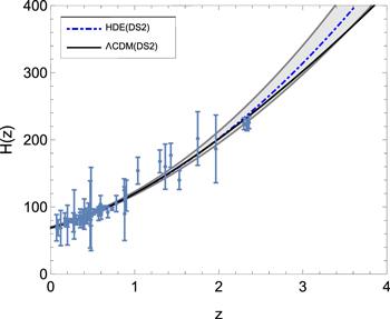
Figure 3. Plot of the Hubble function as a function of redshift for viscous HDE model with bulk viscosity for DS2 dataset over H(z) points and its comparison with ΛCDM model (solid black line). The 57 H(z) data points are also shown with error bars in blue dots. The band corresponds to the error at the 95.4% confidence level. |
The present values of the Hubble constant obtained from DS1 and DS2 are ${H}_{0}={71.567}_{-0.848}^{+1.448}$ and ${H}_{0}={69.197}_{-1.924}^{+1.563}$, respectively. The first value of H0 is slightly lower than the value obtained by SH0ES project H0 = 73.5 ± 1.4 km s−1Mpc−1 [92] whereas the second result of H0 is slightly higher than Planck result [94], where H0 = 67.7 ± 0.46 km s−1Mpc−1. The respective χ2 with DS1 and DS2 data sets are 525.033 and 525.473.
The reduced χ2 statistics are very beneficial in the goodness of fit testing. It is defined as ${\chi }_{\mathrm{red}}^{2}={\chi }_{\min }^{2}/\nu $, where ν is known as the degree of freedom (dof) and is defined as the difference between the total number of combined data points used and the number of estimated free model parameters. We have the number of data points for DS1 as N = 1310 (1048 data of SNe, 57 data of H(z), 204 data of SLS and 01 data of local H0) and for DS2 it is N = 1309 (1048 data of SNe, 57 data of H(z) and 204 data of SLS). The viscous HDE has seven free parameters whereas the ΛCDM has 3. Thus, the ${\chi }_{\mathrm{red}}^{2}$ for ΛCDM comes out to be ${\chi }_{\mathrm{red}}^{2}=0.411$ and ${\chi }_{\mathrm{red}}^{2}=0.406$ whereas for the viscous HDE model, these are ${\chi }_{\mathrm{red}}^{2}=0.402$ and ${\chi }_{\mathrm{red}}^{2}=0.403$, respectively, which is less than unity with each dataset, showing that both the models fit well and data sets are compatible with the considered model.
Table 3 presents the values of transition redshift, the present value of q and ωeff of viscous HDE and ΛCDM models. Figure 4 shows the evolution of the deceleration parameter defined in equation (16 ) for best-fit values of free parameters with the joint datasets. The deceleration parameter shows the transition from q > 0 to q < 0 with both data sets DS1 and DS2. In this cosmological scenario, the signature flipping occurs at the transition redshift ${z}_{\mathrm{tr}}={0.666}_{-0.310}^{+0.426}$ and ${z}_{\mathrm{tr}}={0.777}_{-0.130}^{+0.234}$ corresponding to the DS1 and DS2 datasets, which are very close to the ΛCDM model's transition values. These results are also consistent with the results reported in [95]. Thus, the Universe has a transition from an early decelerated era to the current observable accelerated era. The present value of q(z) is found to be about ${q}_{0}=-{0.535}_{-0.016}^{+0.016}$ and ${q}_{0}=-{0.536}_{-0.016}^{+0.016}$, respectively, which are comparable with ΛCDM and q0 = − 0.55 ± 0.01 of the Planck spacecraft data [94]. It is to be noted that Capozziello et al [96] have obtained q0 = − 0.56 ± 0.04.
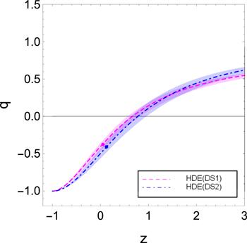
Figure 4. Plot of deceleration parameter q versus redshift z for best-fit values of free parameters obtained from DS1 and DS2 data sets. The current value q0 is shown by a dot on the trajectory. The band corresponds to the error at the 95.4% confidence level. |
Table 3. Values of ${z}_{\mathrm{tr}}$, q0, ωeff(z = 0) and t0 (Gyr) for different combinations of data sets. |
| DS1 | DS2 | |||
|---|---|---|---|---|
| Model | HDE | ΛCDM | HDE | ΛCDM |
| ${z}_{\mathrm{tr}}$ | ${0.666}_{-0.310}^{+0.426}$ | ${0.707}_{-0.205}^{+0.223}$ | ${0.777}_{-0.130}^{+0.234}$ | ${0.699}_{-0.125}^{+0.143}$ |
| q0 | $-{0.535}_{-0.016}^{+0.016}$ | $-{0.568}_{-0.012}^{+0.013}$ | $-{0.536}_{-0.016}^{+0.016}$ | $-{0.563}_{-0.012}^{+0.012}$ |
| ωeff(z = 0) | $-{0.690}_{-0.010}^{+0.010}$ | $-{0.615}_{-0.006}^{+0.006}$ | $-{0.691}_{-0.011}^{+0.011}$ | $-{0.611}_{-0.068}^{+0.068}$ |
Next, we analyze the cosmic expansion using the effective equation of state parameter ωeff. We have plotted the trajectory of ωeff versus redshift z in figure 5, using the best-fit values of free parameters of both the combinations of datasets. The present values of effective EoS parameter are ${\omega }_{\mathrm{eff}}(z=0)=-{0.690}_{-0.010}^{+0.010}$ and ${\omega }_{\mathrm{eff}}(z=0)=-{0.691}_{-0.010}^{+0.010}$ for both; the combination of data sets and their comparison with ΛCDM is listed in table 3. These values are comparatively larger than ω0 = −0.93 which was predicted by joint analysis of WMAP + BAO + H(z) + SNe. The model behaves like quintessence DE. Note that ωeff → −1 in the future time of evolution which implies that the viscous holographic dark energy model approaches to the de Sitter model in late time. Finally, we estimate the age of the Universe as t0 ≈ 13.26 Gyr and t0 ≈ 13.56 Gyr, respectively, which are comparable to the value reported in [94] with t0 = 13.79 ± 0.02 Gyr.
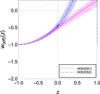
Figure 5. Plot of Effective equation of state parameter ωeff versus redshift z for best-fit values of free parameters obtained from DS1 and DS2 data sets. The current ωeff(z = 0) is shown by a dot on the trajectory. The band corresponds to the error at the 95.4% confidence level. |
5. Diagnostic parameters
In this section, we discuss diagnostic parameters, like statefinder parameters and cosmography parameters, like jerk, snap, lerk, and m parameters to discriminate the proposed viscous HDE model with the dark energy model, like the ΛCDM model.
Sahni et al [97] and Alam et al [98] introduced a new pair of geometrical diagnostic, known as statefinder parameters {r, s} to distinguish the DE models. The pair, using the higher order derivatives of the scale factor, describe the expansion dynamics of the Universe and are defined as15 ) in the above equation, we get
$\begin{eqnarray}r=\displaystyle \frac{1}{{{aH}}^{3}}\displaystyle \frac{{{\rm{d}}}^{3}a}{{{\rm{d}}{t}}^{3}}=\displaystyle \frac{\ddot{H}}{{H}^{3}}-3q-2,\,\,\,s=\displaystyle \frac{r-1}{3(q-1/2)}.\end{eqnarray}$
Now, substituting the values of the scale factor and its derivatives from ( $\begin{eqnarray}\begin{array}{rcl}r & = & \displaystyle \frac{9({1+\alpha {\omega }_{h}-{\xi }_{0}-{\xi }_{1}}^{2})}{{2+3\beta {\omega }_{h}-3{\xi }_{2}}^{2}}{{\rm{e}}}^{-\tfrac{6{\xi }_{0}(t-{t}_{0})}{2+3\beta {\omega }_{h}-3{\xi }_{2}}}\\ & & -9\displaystyle \frac{(1+\alpha {\omega }_{h}-{\xi }_{0}-{\xi }_{1})(1-\alpha {\omega }_{h}+3\beta {\omega }_{h}+{\xi }_{1}-3{\xi }_{2})}{{2+3\beta {\omega }_{h}-3{\xi }_{2}}^{2}}{{\rm{e}}}^{-\tfrac{3{\xi }_{0}(t-{t}_{0})}{2+3\beta {\omega }_{h}-3{\xi }_{2}}}\\ & & +(2+3\beta {\omega }_{h}-3{\xi }_{2}),\end{array}\end{eqnarray}$
and $\begin{eqnarray}\begin{array}{rcl}s & = & \displaystyle \frac{1}{(2+3\beta {\omega }_{h}-3{\xi }_{2})\{2(1+\alpha {\omega }_{h}-{\xi }_{0}-{\xi }_{1})-{{\rm{e}}}^{-\tfrac{3{\xi }_{0}(t-{t}_{0})}{2+3\beta {\omega }_{h}-3{\xi }_{2}}(2+3\beta {\omega }_{h}-2{\xi }_{2})}\}}\\ & & \times \left[2{{\rm{e}}}^{-\tfrac{6{\xi }_{0}(t-{t}_{0})}{2+3\beta {\omega }_{h}-3{\xi }_{2}}}(1+\alpha {\omega }_{h}-{\xi }_{0}-{\xi }_{1})\right.\\ & & \left.\times \{1+\alpha {\omega }_{h}-{\xi }_{0}-{\xi }_{1}-{{\rm{e}}}^{-\tfrac{6{\xi }_{0}(t-{t}_{0})}{2+3\beta {\omega }_{h}-3{\xi }_{2}}}(1+{\xi }_{1}-3{\xi }_{2}-\alpha {\omega }_{h}+3\beta {\omega }_{h})\}\right].\end{array}\end{eqnarray}$
Figure 6 shows the s − r plane trajectories of the viscous holographic dark energy model for best-fit values of parameters achieved through the DS1 and DS2 data. It can be observed that the {r, s} evolutions start from a region of chaplygin gas where r > 1, s < 0 and tends to {r, s} → {1, 0} in future, a value of the ΛCDM model. In figure 6, the horizontal line r = 1 belongs to the ΛCDM model. The present values of the statefinder parameters are {r0 = 0.6415, s0 = 0.132} and {r0 = 0.716, s0 = 0.094} for DS1 and DS2, respectively, which show a deviation from the ΛCDM model. An alternate way to check the differences between the models is through the {q, r} trajectory. In figure 7 we plot such a q − r trajectory for both data sets. The arrow represents the direction of the evolution of the model. The trajectories evolute from deceleration phase to accelerated epoch. We find that {q, r} converges to a steady state (SS) model {−1, 1} in the future (z → −1) with both data sets. In figure 7, the horizontal line at r = 1 belongs to the time evolution of the ΛCDM model.
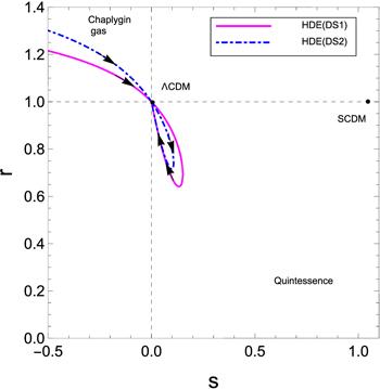
Figure 6. The evolution of {r, s} in s − r plane corresponding to best-fit values of free parameters obtained from DS1 and DS2. The direction of the evolution is shown by the arrows on each trajectory. |
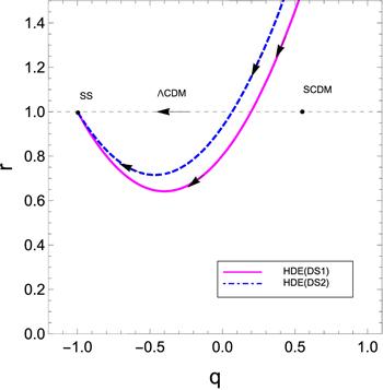
Figure 7. The evolution of {r, q} in q − r plane corresponding to best-fit values of free parameters obtained from DS1 and DS2. |
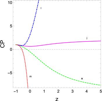
In addition to the above, we report the high order cosmography parameters (jerk, snap, lerk, m) for best-fit values of parameters of the viscous HDE model. These parameters are defined as (see, [99] for historical nomenclature)
$\begin{eqnarray}\begin{array}{rcl}j & = & \displaystyle \frac{1}{{{aH}}^{3}}\displaystyle \frac{{d}^{3}a}{{{dt}}^{3}},\,{\bf{s}}=\displaystyle \frac{1}{{{aH}}^{4}}\displaystyle \frac{{d}^{4}a}{{{dt}}^{4}},\\ l & = & \displaystyle \frac{1}{{{aH}}^{5}}\displaystyle \frac{{d}^{5}a}{{{dt}}^{5}},\,m=\displaystyle \frac{1}{{{aH}}^{6}}\displaystyle \frac{{d}^{6}a}{{{dt}}^{6}}\end{array}\end{eqnarray}$
The jerk parameter provides us the information about the dynamics of the DE. Although the snap, lerk and m parameters do not have a distinguished physical meaning, they are still an important part of the Taylor series of the Hubble parameter and give us more precision in the preferred model. They help to measure the rate of cosmic expansion more accurately.The above cosmographic parameters in terms of redshift are defined as30 ) is different than the one defined in (35 ). Using the best-fit values of model parameters, the evolution of these CP for our model has been shown graphically against redshift, for DS1, and the same can be plotted for the data set DS2.
$\begin{eqnarray}j=-q+(1+z)\displaystyle \frac{{dq}}{{dz}}+2q(1+q),\end{eqnarray}$
$\begin{eqnarray}{\bf{s}}=j-3j(1+q)-(1+z)\displaystyle \frac{{dj}}{{dz}},\end{eqnarray}$
$\begin{eqnarray}l={\bf{s}}-4{\bf{s}}(1+q)-(1+z)\displaystyle \frac{d{\bf{s}}}{{dz}},\end{eqnarray}$
$\begin{eqnarray}m=l-5l(1+q)-(1+z)\displaystyle \frac{{dl}}{{dz}}.\end{eqnarray}$
Here, r and j are the same but the s parameter defined in (The current values of these parameters are found to be {j0 = 0.6415, s0 = − 0.5082, l0 = 3.1301 and m0 = − 14.614} and {j0 = 0.716, s0 = − 0.323, l0 = 2.852 and m0 = − 12.490} for DS1 and DS2 respectively. It can be observed from figure 8 that all the cosmological parameters j, s, l and m tend to unity as z → −1, i.e., our model is in good agreement with the observations of the standard ΛCDM model in late-time evolution. We find that jerk and lerk parameters have trajectories in the same direction while s and m have the same evolution but are different than j and l and both transit from initial negative values to later positive ones. It is also noted that the positive jerk and lerk imply that the Universe has undergone a transition from deceleration to acceleration.
Figure 8. The evolutions of jerk, lerk, snap and m parameters corresponding to best-fit values of model parameters obtained from DS1 and DS2. The direction of the evolution of each trajectory is shown by the arrow. |
6. Conclusion
In this paper, we have studied the effect of bulk viscosity in the HDE model with Granda–Oliveros as an IR cut-off in the framework of FLRW space-time. The viscous term has a negative pressure, therefore, it has been studied to observe the early and late-time accelerated expansion of the Universe. It is well known that the HDE model with the Granda–Oliveros IR cut-off does not show the phase transition which contradicts the present observable Universe. Instead of assuming the other cut-off, we have included a viscous term in the HDE model with the same IR cut-off to observe the phase transition. We have assumed a more general form of the bulk viscous coefficient ξ in terms of H and $\dot{H}$ to demonstrate how the bulk viscosity explains the accelerating Universe. We have obtained the solution of different cosmological parameters such as the Hubble parameter, deceleration parameter and equation of state parameter.
We have constrained the space parameters of the viscous HDE model using the latest observational data of the Strong Lensing system containing 204 data points, H(z) data comprising 57 points, SNe (pantheon data) of 1048 points and local H0. We have performed two joint analyses, namely DS1 and DS2, comprising SLS + SNe + H(z) + H0 and SLS + SNe + H(z), respectively to find the best-fit values of parameters. We have also assumed the ΛCDM model as a concordance model to compare the results of the viscous HDE model. The best-fit values for both models are listed in table 2. Using the best-fit values, we have investigated the effects of bulk viscosity on the evolution of the Universe by plotting the trajectory of different cosmological parameters. We have found that the viscous HDE model fits well to both data sets. We have found a good agreement to data sets according to the ${\chi }_{\mathrm{red}}^{2}$ value. We have also obtained the evolutions of cosmographic parameters and statefinder parameters. In the following, we summarize the main results.
We have plotted and analyzed the trajectory of each of the main observable cosmological parameters such as H(z), q(z) and ωeff(z) using the best-fit values of model parameters. In figures 2 and 3, the Hubble function obtained analytically has been confronted by error bars of Hubble data with best-fit values and compared with ΛCDM. We have found that the model predicts a better fit along with the ΛCDM model. From figures 4 and 5, the evolution of the deceleration and EoS parameters show that the model transits from deceleration phase to the accelerated phase. In late time, we have found that the parameters tend towards −1. The present value of deceleration and EoS parameters are very near to the values of ΛCDM model as mentioned in table 3. The ages of the Universe predicted by the viscous HDE model from two data sets are slightly lower than the value of the ΛCDM model. We have also studied the diagnostic parameters, namely statefinder and cosmographic parameters, for the viscous HDE model, and compared them with the ΛCDM model. Using the best-fit values, we have plotted the evolutions of {r, s}, {r, q} in (s − r), and (q − r) planes, respectively, in figures 6 and 7 and discussed the behavior accordingly. In figure 8, we have plotted the evolution of cosmographic parameters, which explain the dynamics of the model. It has been observed that these parameters tend to 1 as z tends towards −1, that is, the viscous HDE model is in good agreement with the observation of the concordance model in late-time evolution.
The presence of bulk viscosity in dark energy models is an interesting and significant approach to show the phase transition of the Universe. The present model gives a good alternative to explain the accelerating phenomena of the Universe.