


1. Introduction
According to quantum electrodynamics [1-3], the decay dynamics of an excited quantum emitter (QE) can be strongly modified when it is interacting with a tailored electromagnetic field. In the weak coupling regime, the spontaneous emission process is irreversible and is characterized by monotonous exponential decay. But in the strong coupling regime, the decay dynamics change to reversible Rabi oscillations [4]. Besides, we have recently shown that a bound state between a QE and plasmon can be formed [5], where the excited QE will not relax completely to its ground state and is partially stabilized in its excited state after a long time. Coherent control of the decay dynamics plays an important role in quantum computing and quantum state manipulation. Many novel phenomena have been predicted and demonstrated, including Rabi oscillation, quantum entanglement [6], trapping atoms by vacuum forces [7], photon blockade [8, 9], single-molecule sensing [10], single-atom laser [11, 12], enhanced and inhibited spontaneous emission [13-17], and quantum nonlinear optics [18, 19], etc.
Theoretically, the decay dynamics can be accurately studied by solving the Schrödinger equation in the time domain or by the resolvent operator technique in the frequency domain [5, 20]. For the former method, one has to solve the well-known Volterra integral equations of the second kind, which requires the coupling strength over a wide frequency range. In addition, it is not satisfactory from a physical point of view. But for the resolvent operator method, it boasts more obvious physical significance and there is no need for time convolution [5, 21]. However, it requires accurate energy level shift. In recent years, we have developed a fast and accurate universal algorithm for obtaining the energy level shift by using the subtractive Kramers-Kronig (KK) relation [20], which is important for obtaining the exact decay dynamics by the resolvent operator method.
Although both methods can help to obtain accurate decay dynamics, they require the coupling strength over a frequency range [20]. For artificial micro nanostructures, such as photonic crystal microcavity, metal nanoparticles, dimers, etc, the coupling strength can be accurately obtained by many numerical methods, such as the finite difference time domain method [22], finite element method [20, 23-26], and so on. However, these methods are either time-consuming or memory-demanding. For resonant artificial micro-nano structures, the quantized electromagnetic field is usually approximately described by one or several pseudomodes [27-29], where the coupling constant can be semianalytically expressed by a sum of several Lorentzian functions. At this time, the decay dynamics can be easily determined by an effective Hamiltonian. Similar to the case of a QE interacting with a multimode cavity, this allows a simple physical interpretation where the decay dynamics are described in terms of the coupling of the QE to pseudomodes. This effective Hamiltonian method has been widely applied for QE interacting with surface plasmonic nanostructures, including metal nanospheres [16, 30-36], nano dimers [37, 38], metal dielectric interface [15], particle mirror [39, 40], and so on. However, the validity and accuracy of this method are still unclear.
In this work, taking the decay dynamics of a two-level QE near a metal nanosphere as an example, we systematically study the accuracy and validity of the effective Hamiltonian method under different coupling strengths and detunings. The results of the rigorous resolvent operator technique are used as a reference. The content is organized as follows: in section 2 , the model and parameters are introduced, followed by the explanation of the resolvent operator technique and the effective Hamiltonian method. Section 3 shows the accuracy of the effective Hamiltonian method when the system is on resonance. The strong coupling regime and weak coupling regime are considered. Then, the performance of the effective Hamiltonian method under off-resonant conditions is studied, especially when the system has a bound state. Finally, a summary is given in section 4 .
2. Model and method
2.1. Model
As shown in figure 1, there is a two-level QE located near a gold nanosphere of radius a. The excited (ground) state for the QE is denoted as ∣e⟩ (∣g⟩), and the transition frequency is ω0. The matrix element for the transition dipole moment is assumed to be polarized along the radial direction of the sphere, i.e. ${\boldsymbol{d}}={\rm{d}}\,\hat{{\boldsymbol{r}}}$, and its strength is d = 24 D. Without specification, we set a = 20 nm and h = 1 nm. The background is a vacuum with ϵ1 = 1. The relative electric permittivity of Gold is described by the Drude model [41-44], ${\varepsilon }_{2}(\omega )\,=1-{\omega }_{p}^{2}/[\omega (\omega +{\rm{i}}{\gamma }_{p})]$ with ωp = 1.26 × 10¹⁶ rad s−1 and γp = 1.41 × 10¹⁴ rad s−1.
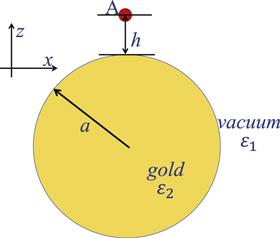
Figure 1. Schematic diagrams. A QE is located around a gold nanosphere with radius a. The distance between the QE and the surface of the nanosphere is h. ϵ1 and ϵ2 are the permittivities for vacuum and metal, respectively. |
2.2. The resolvent operator technique
By macroscopic quantum electrodynamics, the quantized electromagnetic field in the presence of dispersing and absorbing dielectric bodies can be expressed in terms of a bosonic polaritonic vector field operator [29]. Initially, the two-level QE is in an excited state, and the medium-assisted field is in a vacuum state. Under the dipole approximation and the rotating-wave approximation [45, 46], the probability amplitude for the QE in the excited state can be derived from Green's function expression of the evolution operator [5, 20, 26]. Explicitly, it reads
$\begin{eqnarray}{c}_{1}(t)={\int }_{-\infty }^{+\infty }S(\omega ){{\rm{e}}}^{-{\rm{i}}\omega t}{\rm{d}}\omega ,\end{eqnarray}$
with the evolution spectrum $\begin{eqnarray}S(\omega )=\displaystyle \frac{1}{\pi }\mathop{\mathrm{lim}}\limits_{\eta \to {0}_{+}}\displaystyle \frac{{\rm{\Gamma }}(\omega )/2+\eta }{{\left[\omega -{\omega }_{0}-{\rm{\Delta }}(\omega )\right]}^{2}+{\left[{\rm{\Gamma }}(\omega )/2+\eta \right]}^{2}},\end{eqnarray}$
where Δ(z) and Γ(z) represent the analytic part and the non-analytic part of the self-energy, respectively [47, 48], which can be written as $\begin{eqnarray}{\rm{\Gamma }}(z)=2\pi \mathrm{Im}{g}_{{rr}}(z)\theta (z),\end{eqnarray}$
$\begin{eqnarray}{\rm{\Delta }}(z)={\mathbb{P}}{\int }_{0}^{+\infty }{\rm{d}}s\displaystyle \frac{\mathrm{Im}{g}_{{rr}}(s)}{z-s}.\end{eqnarray}$
Here, θ(z) is the step function. g(ω) is the coupling strength, which can be expressed by the classical photon Green's function (GF) $\begin{eqnarray}{g}_{{rr}}(\omega )=\displaystyle \frac{{{\boldsymbol{d}}}^{* }\cdot {\boldsymbol{G}}({{\boldsymbol{r}}}_{0},{{\boldsymbol{r}}}_{0},\omega )\cdot {\boldsymbol{d}}}{{\hslash }\pi {\varepsilon }_{0}}.\end{eqnarray}$
Here, the photon GF satisfies $\begin{eqnarray}\begin{array}{l}{\rm{\nabla }}\times {\rm{\nabla }}\times {\boldsymbol{G}}\left({\boldsymbol{r}},{{\boldsymbol{r}}}_{0},\omega \right)-\varepsilon ({\boldsymbol{r}},\omega )\\ \quad \times \,\displaystyle \frac{{\omega }^{2}}{{c}^{2}}{\boldsymbol{G}}\left({\boldsymbol{r}},{{\boldsymbol{r}}}_{0},\omega \right)=\displaystyle \frac{{\omega }^{2}}{{c}^{2}}{\boldsymbol{I}}\delta ({\boldsymbol{r}}-{{\boldsymbol{r}}}_{0}).\end{array}\end{eqnarray}$
In the case of a weak coupling regime, Δ(ω0) and Γ(ω0) represent the energy level shift and the spontaneous emission rate, respectively. For the energy level shift Δ(ω) (equation (4 )), the photon GF over a much wide frequency range is needed for the evaluation of the principal value integral. It should be noted that numerical evaluation of the photon GF is not an easy task for an arbitrary-shaped nanostructure. In recent years, we have developed a fast and accurate method to calculate the energy level shift using the subtractive KK relation [5, 20]. When ω > 0, the energy level shift can be written as4 ), this expression avoids the principal value integral, and the integrand decays faster. It has been shown in [20] that it is over a narrow frequency range that the energy level shift Δ(ω) can be obtained by equation (7 ).
$\begin{eqnarray}\begin{array}{rcl}{\rm{\Delta }}\left(\omega \right) & = & -\pi \mathrm{Re}{g}_{{rr}}\left(\omega \right)+\displaystyle \frac{\pi }{2}\mathrm{Re}{g}_{{rr}}\left(0\right)\\ & & -\omega {\int }_{0}^{+\infty }{\rm{d}}s\displaystyle \frac{\mathrm{Im}{g}_{{rr}}\left(s\right)}{\left(\omega +s\right)s}.\end{array}\end{eqnarray}$
Compared with equation (Thus, to evaluate the probability amplitude of the excited state by the rigorous resolvent operator technique (equation (1 )), it is necessary to first calculate the photon GF ${\boldsymbol{G}}\left({{\boldsymbol{r}}}_{0},{{\boldsymbol{r}}}_{0},z\right)$. Then, from equations (3 ) and (7 ), we can obtain Γ(ω) and Δ(ω). Substituting them into equation (2 ), we can obtain the evolution spectrum S(ω) and then the probability amplitude of the excited state c1(t) by Fourier transformation (equation (1 )).
The core of the above steps is to find the photon GF. For the nanosphere, the photon GF has a semi-analytic solution [23]. The radial component of the scattering GF is
$\begin{eqnarray}z\cdot {{\boldsymbol{G}}}_{s}\left({{\boldsymbol{r}}}_{0},{{\boldsymbol{r}}}_{0},\omega \right)\cdot z=\displaystyle \sum _{n=1}^{\infty }{G}_{n}\left({{\boldsymbol{r}}}_{0},{{\boldsymbol{r}}}_{0},\omega \right),\end{eqnarray}$
where Gn refers to the contribution of the nth plasmon. Explicitly, it reads $\begin{eqnarray}\begin{array}{l}{G}_{n}\left({{\boldsymbol{r}}}_{0},{{\boldsymbol{r}}}_{0},\omega \right)=\displaystyle \frac{{\rm{i}}{k}^{2}{k}_{1}}{4\pi \,}{R}^{V}\\ \quad \times \,(2n+1)n(n+1){\left[\displaystyle \frac{{h}_{n}^{(1)}({k}_{1}{r}_{0})}{{k}_{1}{r}_{0}}\right]}^{2},\end{array}\end{eqnarray}$
in which, k = ω/c, and ${k}_{i}=\omega \sqrt{{\varepsilon }_{i}}/c$. ϵ1 and ϵ2 are the dielectric functions of the background and metal, respectively. ${h}_{n}^{(1)}$ is the spherical Hankel function of the first kind. ${r}_{0}=\left|{{\boldsymbol{r}}}_{0}\right|$ is the distance from the quantum dot to the center of the nanosphere. RV is the reflection coefficient given by $\begin{eqnarray}{R}^{V}=\displaystyle \frac{{k}_{2}{\tau }_{2}\partial {\tau }_{1}-{k}_{1}{\tau }_{1}\partial {\tau }_{2}}{{k}_{2}{\tau }_{2}\partial {\kappa }_{1}-{k}_{1}{\kappa }_{1}\partial {\tau }_{2}}.\end{eqnarray}$
Here, τi = ρijn(ρi) and ${\kappa }_{i}={\rho }_{i}{h}_{n}^{(1)}({\rho }_{i})$ are the Riccati-Bessel function and Riccati-Hankel function with ρi = kia, respectively. $\partial {\tau }_{i}={\left.\tfrac{{\rm{d}}[\rho {j}_{n}(\rho )]}{{\rm{d}}\rho }\right|}_{\rho ={\rho }_{i}}$ and $\partial {\kappa }_{i}={\left.\tfrac{{\rm{d}}[\rho {h}_{n}^{(1)}(\rho )]}{{\rm{d}}\rho }\right|}_{\rho ={\rho }_{i}}$ are their derivatives.2.3. Effective Hamiltonian method
Effective Hamiltonian can be derived, if the coupling constant
$\begin{eqnarray}{\left|{\kappa }_{n}\left(\omega ,{{\boldsymbol{r}}}_{0}\right)\right|}^{2}=\mathrm{Im}{g}_{{rr}}(\omega ),\end{eqnarray}$
between the two-level QE and each surface plasmon resonance of the nanosphere can be approximated by a Lorentzian profile [33] $\begin{eqnarray}{\left|{\kappa }_{n}\left(\omega ,{{\boldsymbol{r}}}_{0}\right)\right|}^{2}=\displaystyle \frac{{g}_{n}^{2}({{\boldsymbol{r}}}_{0})}{\pi }\displaystyle \frac{{\gamma }_{n}/2}{{\left(\omega -{\omega }_{n}\right)}^{2}+\tfrac{{\gamma }_{n}^{2}}{4}}.\end{eqnarray}$
Here, gn is the coupling strength between the QE and the n-th plasmon. ωn and γn are the plasmon resonance frequency and width, respectively. In the basis { $\left|e\right\rangle \left|\varnothing \right\rangle $, $\left|g\right\rangle \left|{1}_{1}\right\rangle $, ⋯, $\left|g\right\rangle \left|{1}_{N}\right\rangle $ }, the matrix representation of the effective Hamiltonian reads [33] $\begin{eqnarray}{H}_{\mathrm{eff}}={\hslash }\left[\begin{array}{ccccc}-{\rm{i}}\displaystyle \frac{{\gamma }_{d}}{2} & {\rm{i}}{g}_{1} & {\rm{i}}{g}_{2} & \cdots & {\rm{i}}{g}_{N}\\ -{\rm{i}}{g}_{1} & {{\rm{\Delta }}}_{1}-{\rm{i}}\displaystyle \frac{{\gamma }_{1}}{2} & 0 & \cdots & 0\\ -{\rm{i}}{g}_{2} & 0 & {{\rm{\Delta }}}_{2}-{\rm{i}}\displaystyle \frac{{\gamma }_{2}}{2} & \ddots & \vdots \\ \vdots & \vdots & \ddots & \ddots & 0\\ -{\rm{i}}{g}_{N} & 0 & \cdots & 0 & {{\rm{\Delta }}}_{N}-{\rm{i}}\displaystyle \frac{{\gamma }_{N}}{2}\end{array}\right],\end{eqnarray}$
where Δn = ωn − ω0 is the detuning of the nth plasmon resonance from the QE transition frequency, γd is the intrinsic nonradiative decay rate of the QE, which is γd = 0 in our system.The decay dynamics is determined by the above effective Hamiltonian whose eigenvalues and eigenvectors satisfy
$\begin{eqnarray}{H}_{\mathrm{eff}}\left|{{\rm{\Pi }}}_{m}^{R}\right\rangle ={\lambda }_{m}\left|{{\rm{\Pi }}}_{m}^{R}\right\rangle .\end{eqnarray}$
Then, the solution of the Schrödinger equation ${\rm{i}}{\hslash }{\partial }_{t}\left|\psi (t)\right\rangle ={H}_{\mathrm{eff}}\left|\psi (t)\right\rangle $ can be written as $\begin{eqnarray}\left|\psi (t)\right\rangle =\displaystyle \sum _{m=1}^{N+1}{\eta }_{m}\left|{{\rm{\Pi }}}_{m}^{R}\right\rangle {{\rm{e}}}^{-{\rm{i}}{\lambda }_{m}t}.\end{eqnarray}$
Here, ${\eta }_{m}=\left\langle {{\rm{\Pi }}}_{m}^{L}| \psi (0)\right\rangle $, and $\left|{{\rm{\Pi }}}_{m}^{L}\right\rangle $ is the eigenvector of ${H}_{\mathrm{eff}}^{\dagger }$ and satisfies the orthogonal normalization condition, i.e. ${H}_{\mathrm{eff}}^{\dagger }\left|{{\rm{\Pi }}}_{m}^{L}\right\rangle ={\lambda }_{{}_{m}}^{* }\left|{{\rm{\Pi }}}_{m}^{L}\right\rangle $ and $\left\langle {{\rm{\Pi }}}_{m}^{L}| {{\rm{\Pi }}}_{m}^{R}\right\rangle ={\delta }_{{mn}}$. If $\left|{{\rm{\Pi }}}_{m}^{R}\right\rangle ={m}_{0}\left|{\rm{e}}\right\rangle \left|\varnothing \right\rangle +{\sum }_{n=1}^{N}{m}_{n}\left|{\rm{g}}\right\rangle \left|{1}_{n}\right\rangle $, then one has $\left|{{\rm{\Pi }}}_{m}^{L}\right\rangle =-{m}_{0}^{* }\left|{\rm{e}}\right\rangle \left|\varnothing \right\rangle \,+{\sum }_{n=1}^{N}{m}_{n}\left|{\rm{g}}\right\rangle \left|{1}_{n}\right\rangle $. For our system with the QE initially in the excited state and the medium-assisted field in the vacuum state, i.e. $\left|\psi (0)\right\rangle =\left|{\rm{e}}\right\rangle \left|\varnothing \right\rangle $, the probability that the QE remains in the excited state can be expressed as $\begin{eqnarray}{\left|{c}_{e}(t)\right|}^{2}={\left|\,\left\langle {\rm{e}},\varnothing | \psi (t)\right\rangle \,\right|}^{2}={\left|\displaystyle \sum _{m=1}^{N+1}{m}_{0}^{2}{{\rm{e}}}^{-{\rm{i}}{\lambda }_{m}t}\right|}^{2}.\end{eqnarray}$
In this method, first of all, the resonant frequency ωn and width γn of the plasmon, and the coupling strength gn must be solved to construct the effective Hamiltonian (equation (13 )). Then, the eigenvalues λm and normalized eigenvectors $\left|{{\rm{\Pi }}}_{m}^{R}\right\rangle ={m}_{0}\left|{\rm{e}}\right\rangle \left|\varnothing \right\rangle +{\sum }_{n=1}^{N}{m}_{n}\left|{\rm{g}}\right\rangle \left|{1}_{n}\right\rangle $ can be obtained. Finally, from equation (16 ), the decay dynamics can be obtained.
The core of the above steps is to solve the relevant parameters ωn, γn and gn. For metallic nanosphere, there are two ways to obtain them. One method is to calculate the coupling constants ${\left|{\kappa }_{n}\left(\omega ,{{\boldsymbol{r}}}_{d}\right)\right|}^{2}$ at different frequency points, which can be used to deduce the above parameters from a Lorentz fit (equation (12 )). The other method is to directly find the complex resonant frequencies of the surface plasmon Ωn by performing an analytical continuation of Gn to the complex frequency plane. The poles of Gn are determined by the zeros of the denominator for the reflection coefficients RV (equation (10 )). Then, the resonant frequency ωn and width γn are the real part and imaginary part, respectively, i.e. Ωn = ωn − iγn/2. From equation (12 ), the coupling strength can be expressed as ${g}_{n}({{\boldsymbol{r}}}_{d})=\left|{\kappa }_{n}\left({\omega }_{n},{{\boldsymbol{r}}}_{d}\right)\right|\sqrt{\pi {\gamma }_{n}/2}$ when ω = ωn, so that only the imaginary part of the photon GF $\mathrm{Im}\left[{{\boldsymbol{G}}}_{n}\left({{\boldsymbol{r}}}_{d},{{\boldsymbol{r}}}_{d},{\omega }_{n}\right)\right]$ at ωn should be calculated.
We have numerically proved that both methods give almost the same results for the system investigated in this paper. It should be noted that the computational resource required by the first method is much larger than that by the second method. For the first method where the parameters are deduced from a Lorentzian fit, the photon GF at a large number of frequency points should be calculated. But for the second method, it is only at a single frequency point that the photon GF should be calculated. As stated in [20], numerical evaluation of the photon GF is not an easy task, especially for an arbitrary-shaped nanostructure.
According to equations (3 ) and (11 ), we have ${\rm{\Gamma }}(\omega )\,=2\pi {\sum }_{n=1}^{N}{\left|{\kappa }_{n}\left(\omega ,{{\boldsymbol{r}}}_{d}\right)\right|}^{2}$. Under the pseudomode approximation (equation (12 )), the spontaneous emission rate can be written as4 ) and extending the lower limit of integration from zero to −∞, the approximate energy level shift can be obtained analytically and reads
$\begin{eqnarray}{{\rm{\Gamma }}}_{\mathrm{eff}}(\omega )=\displaystyle \sum _{n=1}^{N}\displaystyle \frac{{g}_{n}^{2}{\gamma }_{n}}{{\left(\omega -{\omega }_{n}\right)}^{2}+{\left({\gamma }_{n}/2\right)}^{2}}.\end{eqnarray}$
Substituting it into equation ( $\begin{eqnarray}{{\rm{\Delta }}}_{\mathrm{eff}}(\omega )=\displaystyle \sum _{n=1}^{N}\displaystyle \frac{{g}_{n}^{2}(\omega -{\omega }_{n})}{{\left(\omega -{\omega }_{n}\right)}^{2}+{\left({\gamma }_{n}/2\right)}^{2}}.\end{eqnarray}$
3. Results and discussion
Figure 2 shows the spontaneous emission rate Γ(ω) and energy level shift Δ(ω) obtained by using the exact photon GF expression and by the pseudomode approach. For the spontaneous emission rate Γ(ω), see figure 2(a), the black solid line is the result obtained by the strict photon GF (equation (9 )), and the red dashed line is the result under the pseudomode approximation (equation (17 )). It can be seen that the two methods give almost the same Γ(ω). For frequency away from the resonance, see the inset, the approximate method (red dashed line) predicts a slightly higher value than that by the strict solution (black solid line). This can be understood as follows. For the approximate method, see equation (17 ), Γeff(ω) converges to a non-zero value when ω → 0. However, it should converge to zero since a static dipole moment does not radiate electromagnetic waves.

Figure 2. Spontaneous emission rate Γ(ω) and level shift Δ(ω) change with frequency (ω). In (a), Γ(ω) is a function of frequency (ω), the black solid line represents the result obtained from the exact solution of photon Green's function Γdir(ω), and the red dashed line is Γeff(ω) obtained by approximated pseudomodes. In (b), Δ(ω) is a function of frequency (ω), the black solid line is ΔKK(ω) obtained by subtracting the KK relationship, and the red dashed line is Δeff(ω) obtained by approximated pseudomodes. |
It is worth noting that although Γ(ω) exhibits almost a single peak located near ωc = 5.8 eV, there are 250 plasmon modes to obtain a convergent result. Due to the short distance between the QE and the nanosphere, the higher-order modes contribute greatly, and their resonance frequencies are concentrated at ωc.
For the energy level shift Δ(ω), see figure 2(b), where the black solid line indicates the exact solution using the subtractive KK relation method (equation (7 )), and the red dashed line is the energy level shift Δeff(ω) under the pseudomode approximation (equation (18 )). Over a wide frequency range, the two methods give similar Δ(ω). As shown in the inset, we can see an error $\left|{{\rm{\Delta }}}_{\mathrm{eff}}(\omega )-{{\rm{\Delta }}}_{\mathrm{KK}}(\omega )\right|$ at about 0.04 eV. This is mainly due to the fact that the strict method (equation (7 )) takes into account the quantum corrections and the contribution of all non-resonant modes, while the pseudomode-approximated method (equation (18 )) only takes into account the contribution of resonant modes and neglects quantum corrections (extending the lower limit of integration from zero to −∞).
We first study the decay dynamics at resonance. In this case, the transition frequency of the QE is ω0 = 5.8 eV, which is the peak frequency in figure 2(a). As shown in figure 3(a), the red hollow circles represent the rigorous solution by the resolvent operator method, where Γ(ω) and Δ(ω) are obtained from equations (3 ) and (7 ) using the exact photon GF, and the survival probabilities of the excited states is obtained by equations (1 ) and (2 ). The green solid line is the result obtained by the effective Hamiltonian method, i.e. the survival probability of the excited states obtained by equation (16 ), which is in good agreement with the rigorous solution (red hollow circle). This clearly shows that the effective Hamiltonian method can accurately solve the dynamics at resonance.

Figure 3. Evolution of the excited state population ${P}_{a}\left(t\right)={\left|{c}_{1}\left(t\right)\right|}^{2}$ with the variable t. The transition frequency ω0 = 5.8 eV, and the transition dipole moment d = 24 D. The results obtained by the resolvent operator method and the effective Hamiltonian method are compared, and the results agree well. The inset shows the results of a smaller time. In (a), the green solid line is the result obtained by the effective Hamiltonian method, and the red hollow circle is the result obtained by the rigorous resolvent operator method. The blue triangle is the result obtained by Γeff(ω) and Δeff(ω) is used in the resolvent operator method. In (b), the red hollow circle is the result obtained by ΔKK(ω) and Γeff(ω). The blue triangle is the result obtained by Δeff(ω) and Γdir(ω). The green solid line is the result obtained by the effective Hamiltonian method. |
It is worth noting that the computation time required by the effective Hamiltonian method is much shorter than that by the rigorous resolvent operator method. For both methods, almost all of the computation time is spent in the evaluation of the photon GF Gn. For the effective Hamiltonian method, only at a single frequency point ωn should the imaginary part of photon GF Gn (equation (9 )) be calculated for each plasmon mode. But for the rigorous resolvent operator method, we have to calculate the photon GF Gn at thousands of frequency points to properly describe its distribution. In this work, 3000 frequency points are used for each plasmon mode.
As stated in section 2 , approximate Γ(ω) and Δ(ω), i.e. Γeff(ω) (equation (17 )) and Δeff(ω) (equation (18 )), may also be used in the resolvent operator method. See figure 3(a), the results (blue triangle) are also in good agreement with the rigorous solution (red hollow circle), indicating that contributions from the non-resonance and quantum correction effects are very small and can be ignored at resonance. When only approximate Γeff(ω) or approximate Δeff(ω) is used, see figure 3(b), the results are in good agreement with that of the effective Hamiltonian method. Thus, approximate Γ(ω) (equation (17 )) and Δ(ω) (equation (18 )), and accordingly the effective Hamiltonian method can be applied at resonance.
From the above results, we can conclude that the effective Hamiltonian method gives accurate dynamics when the transition frequency of the QE is near the surface plasmon resonance. It needs much fewer computation resources than that of the resolvent operator method. In addition, the resolvent operator method using Γeff(ω) and Δeff(ω) also gives accurate decay dynamics at resonance, which shows that neither non-resonance part nor quantum correction takes effect.
In the above case, the QE oscillates back and forth between the excited and ground states (Rabi oscillation), showing a strong coupling characteristic. Next, we study the weak coupling case. To this end, we increase the distance between the QE and the nanosphere and set h = 5 nm. At this time, the spontaneous emission rate Γ(ω) and energy level shift Δ(ω) are shown in figures 4(a) and (b), respectively. Similar to figure 2, the spontaneous emission rate Γ(ω) and level shift Δ(ω) obtained under the pseudomode approximation are similar to those obtained by the exact photon GF (equation (17 )). Compared to the results in figure 2, the peak values for Γ(ω) and Δ(ω) are small, and there are multiple peaks for Γ(ω). This is mainly due to the fact that the surface plasmon electric field decreases sharply with increasing distance, and drops faster for higher-order modes [23]. Thus, it is gradually becoming more important for lower-order modes. The first peak at 4.41 eV is due to the contribution of the dipolar surface plasmon resonance (n = 1) since the real part for the zero of the denominator of RV is 4.41 eV at n = 1.
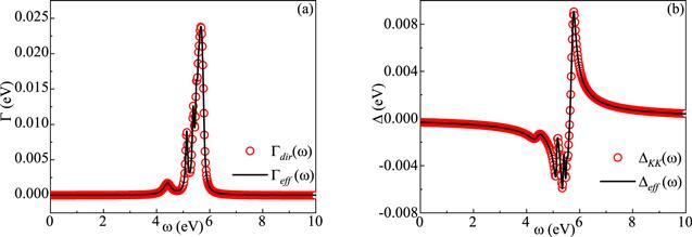
Figure 4. Spontaneous emission rate Γ(ω) and level shift Δ(ω) change with frequency (ω), the distance between the QE and the surface of the nanosphere is h = 5 nm. In (a), Γ(ω) is a function of frequency (ω), the red hollow circle is Γdir(ω), and the black solid line is Γeff(ω). In (b), Δ(ω) is a function of frequency (ω), the red hollow circle is ΔKK(ω), and the black solid line line is Δeff(ω). |
Assuming that the transition frequency of the QE is equal to the dipolar resonate frequency, i.e. ω0 = 4.41 eV, we plot the decay dynamics in figure 5. The effective Hamiltonian method can also give accurate results, which is similar to the strong coupling case shown in figure 3. Besides, when the spontaneous emission rate Γ(ω) and energy level shift Δ(ω) under the pseudomode approximation are used in the resolvent operator method, the results (blue triangle) are also in good agreement with the reference solution.
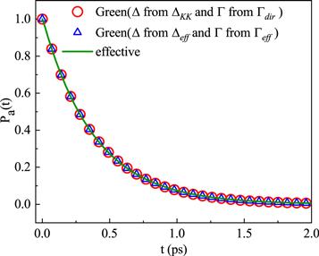
Figure 5. Evolution of the excited state population ${P}_{a}\left(t\right)={\left|{c}_{1}\left(t\right)\right|}^{2}$ with the variable t. The transition frequency ω0 = 4.41 eV, and the transition dipole moment d = 24 D. The results obtained by the resolvent operator method and effective Hamiltonian method are compared. The green solid line is the result obtained by the effective Hamiltonian method, and the red hollow circle is the result obtained by the rigorous resolvent operator method. The blue triangle is the result obtained by Γeff(ω) and Δeff(ω) are used in the resolvent operator method. The results agree well. Here, the distance between the QE and the surface of the nanosphere is h = 5 nm. |
Then, we turn to investigate the decay dynamics when the transition frequency is off-resonant with the surface plasmon. As an example, we set ω0 = 1.5 eV, which is much smaller than the mode resonance frequency. From figure 6(a), one can see that the decay dynamics by the effective Hamiltonian method (red hollow circle) differ much from the rigorous results obtained by Green's function resolvent operator method (purple dashed line). The effective Hamiltonian method overestimates the spontaneous emission rate. In the weak coupling regime, the spontaneous emission rate is nearly equal to Γ(ω) when ω is around ω0 = 1.5 eV. Similar to the results shown in the inset in figure 2(a), Γ(ω0) obtained by the pseudomode approximation (Γeff) is larger than that by the rigorous photon GF (Γdir), which gives a clear understanding of the faster decaying for the effective Hamiltonian method.
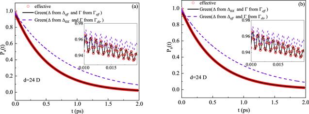
Figure 6. Evolution of the excited state population ${P}_{a}\left(t\right)={\left|{c}_{1}\left(t\right)\right|}^{2}$ with the variable t, here ω0 = 1.5 eV, and d = 24 D. The results obtained by the resolvent operator method and the effective Hamiltonian method are compared. In (a), the red hollow circle is the result obtained by the effective Hamiltonian method, and the black solid line is the result obtained by Γeff(ω) and Δeff(ω) are used in the resolvent operator method. The purple dashed line is the result obtained by ΔKK(ω) and Γdir(ω). In (b), the red hollow circle is the result obtained by the effective Hamiltonian method, the black solid line is the result obtained by ΔKK(ω) and Γeff(ω). The purple dashed line is the result obtained by Δeff(ω) and Γdir(ω). The inset shows the results of a shorter time. |
However, if the approximate spontaneous emission rate Γeff(ω) and energy level shift Δeff(ω) are used in the resolvent operator method, the decay dynamics (solid black line) are the same as those obtained by the effective Hamiltonian method (red hollow circle). This means that the resolvent operator method is equivalent to the effective Hamiltonian method once Γeff(ω) and Δeff(ω) are used. The main reason why the decay dynamics by the effective Hamiltonian method deviates from the strict solution comes from the pseudomode approximation, i.e. Γeff(ω) and Δeff(ω).
To further determine how Γeff(ω) and Δeff(ω) affect the decay dynamics, we plot the results in figure 6(b) when either Γeff(ω) (black solid line) or Δeff(ω) (purple dashed line) is used. It can be seen that the results from the approximated spontaneous emission rate Γeff(ω) and the exact energy level shift Δ(ω) are in rather good agreement with those by the effective Hamiltonian method. This means that the decay dynamics are not affected by using Δeff(ω) in the off-resonant case. However, the results by using exact spontaneous emission rate Γ(ω) and approximated energy level shift Δeff(ω) are different from those by the effective Hamiltonian method, which means that the exact spontaneous emission rate plays an important role.
The above phenomena also exist for other non-resonant frequencies. Figure 7 shows the results for ω0 = 3.5 eV, which is a little lower than the dipolar plasmon frequency ω1 = 4.41 eV. Results by using the effective Hamiltonian method are the same as those by the Green's function resolvent operator when using Γeff(ω) [black solid line in figure 7(a)], but are different from the strict solution by using exact Γ(ω) (purple dashed line in figure 7(a)). From figure 7(b), one can see that the red hollow circles obtained by the effective Hamiltonian method are located on the black solid line which represents the results using the exact Δ(ω). Thus, we can also conclude that the decay dynamics are not affected by using approximated energy level shift Δeff(ω).
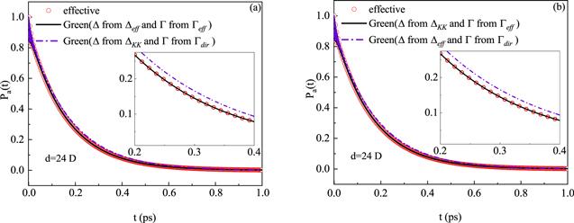
Figure 7. Evolution of the excited state population ${P}_{a}\left(t\right)={\left|{c}_{1}\left(t\right)\right|}^{2}$ with the variable t, here ω0 = 3.5 eV, and d = 24 D. The results obtained by the resolvent operator method and the effective Hamiltonian method are compared. In (a), the red hollow circle is the result obtained by the effective Hamiltonian method, and the black solid line is the result obtained by Γeff(ω) and Δeff(ω) is used in the resolvent operator method. The purple dashed line is the result obtained by ΔKK(ω) and Γdir(ω). In (b), the red hollow circle is the result obtained by the effective Hamiltonian method, the black solid line is the result obtained by ΔKK(ω) and Γeff(ω). The purple dashed line is the result obtained by Δeff(ω) and Γdir(ω). The inset shows the results of a shorter time. |
The above results show that the effective Hamiltonian method can accurately describe the decay dynamics when the transition frequency of the QE is in resonance with the plasmon. However, it has some limitations when the transition frequency is far away from the resonance frequency of the surface plasmon. The error can be attributed to the approximated spontaneous emission rate Γeff(ω). The decay dynamics are nearly not affected by using approximated energy level shift Δeff(ω).
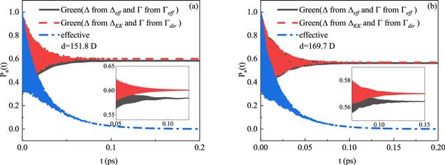
In the following of this work, we consider a special case where a bound state between QE and surface plasmon polaritons is formed. The excited QE will not relax completely to its ground state and is partially stabilized in its excited state after a long time [5, 49]. We have shown in [5] that a bound state exists when the dipole moment d of the QE is larger than a critical value ${d}_{c}={\left[2{\hslash }{\varepsilon }_{0}{\omega }_{0}/(\hat{{\boldsymbol{r}}}\cdot \mathrm{Re}{\boldsymbol{G}}\left({{\boldsymbol{r}}}_{0},{{\boldsymbol{r}}}_{0},0\right)\cdot \hat{{\boldsymbol{r}}})\right]}^{1/2}$. For our system, the critical transition dipole moment is dc = 140.3 D when ω0 = 1.5 eV. We consider two different dipole moments d = 151.8 D and d = 169.7 D, which are larger than the critical value dc. For both cases shown in figure 8, the resolvent operator method gives the bound state characteristics, i.e. the survival probability of the excited state does not decay to zero in the long time limit, while the effective Hamiltonian method predicts zero survival probability in the long time limit. This is mainly due to the fact that the eigenvalues for the effective Hamiltonian are all complex numbers and then the survival probability of the excited state eventually decays to 0 by equation (16 ). Thus, the effective Hamiltonian method cannot be applied when a bound state exists.
Figure 8. Evolution of the excited state population ${P}_{a}\left(t\right)={\left|{c}_{1}\left(t\right)\right|}^{2}$ with the variable t. When a bound state between QE and surface plasmon polaritons is formed, the results obtained by the resolvent operator method and the effective Hamiltonian method are compared. (a) shows the results for ${P}_{a}\left(t\right)$ with d = 151.8 D, the black solid line is the result obtained by Γeff(ω) and Δeff(ω) are used in the resolvent operator method, and the red dashed line is the result obtained by ΔKK(ω) and Γdir(ω). The blue dashed line is the result obtained by the effective Hamiltonian method. (b) shows the results for ${P}_{a}\left(t\right)$ with the transition dipole moment d = 169.7 D. |
4. Conclusion
In this investigation, the applicability and accuracy of the effective Hamiltonian method for decay dynamics are systematically investigated. It gives accurate results when the QE is resonant with the plasmon regardless of the strength of the coupling. However, the effective Hamiltonian method is not accurate in the case of large detuning. We have found that the errors are not from the approximation made on the energy level shift Δ(ω), but from the approximation made on the spontaneous emission rate, i.e. using Γeff(ω). The smaller the difference between the approximated spontaneous emission rate Γeff(ω) and the accurate one Γ(ω), the smaller the errors are. Besides, the effective Hamiltonian method cannot be applied when there is a bound state between the QE and plasmon. These results provide guidance for the application of the effective Hamiltonian method based on pseudomode theory.