


1. Introduction
It is well known that quantum computation and information use quantum mechanical systems to effectively accomplish powerful computational and informational tasks [1]. Despite many claims, quantum computation is not always more efficient than classical computation in specific operations. The operations that are not possible to complete are referred to as ‘no-go theorems' in the description of the quantum realm. Several well-known no-go theorems like the no-cloning theorem [2, 3], no-deletion theorem [4, 5], no-splitting theorem [6], no-flipping theorem [7], and no-partial erasure [8] are introduced in various contexts.
Among the no-go theorems, the impossibility of ideal cloning and ideal deletion are two essential theorems on quantum information theory constrained by nature. The linearity of quantum theory reveals that it is impossible to precisely replicate an unknown quantum state [2, 3]. The unitarity nature of quantum evolution demonstrates that the ideal copies of non-orthogonal quantum states are impossible [9]. However, a unitary and measurement process can feasibly create a quantum cloning machine that replicates an unknown quantum state approximately [10-15]. These probabilistic quantum cloning machines can be divided into two categories. One type is a state-dependent quantum cloning machine, as such a Wootters-Zurek (WZ) quantum cloning machine, where the copying ability is dependent on the input state [2]. The second type is a universal quantum cloning machine, such as a Buzek-Hillery (BH) quantum cloning machine, where for all input states, the ability of copying is the same [10]. On the other side, quantum deletion deals with the impossibility of deleting an arbitrary quantum state [4]. More specifically, it asserts that neither a reversible nor an irreversible deletion of an unknown quantum state from two copies of it is possible due to the linearity of quantum theory. Quantum deletion more closely resembles reversible uncopying of an unknown quantum state [4]. If one attempts to delete an unknown quantum state using the probabilistic method, then it is conceivable with a success probability of less than unity [16]. Different approximation deleting machines (DMs) have been developed by researchers. These are either state-dependent or independent DMs [17-22]. These DMs are imperfect in the sense that they can neither perfectly delete the copy mode nor retain the input state. The no-deleting principle claims that although quantum information cannot be destroyed in a closed system and cannot be properly replicated, it can be moved from one place to another. The no-cloning theorem and the no-deleting theorem are used to develop the law of conservation of quantum information theory, which asserts that information cannot be created or destroyed in the quantum world [23].
By re-exploring the no-deleting theorem, we can better comprehend how it connects to other no-go theorems, which opens up the prospect of gaining fundamental knowledge of the quantum world and it being used in future quantum technology [24]. In this line of thought, we revisit the performance of our prescribed DM [25] and the well-known Pati-Braunstein (PB) DM [4]. We define the operation of the DMs as one shot DMs. In this work, we analyze some important attributes such as the non-violation of Bell's inequalities and the teleportation fidelity of one shot DMs.
In classical computation, it is known that NAND is considered to be a universal gate, as suitable combinations of the NAND gate can generate other basic gates like AND, OR, and NOT. In other words, the concatenation of NAND can realize other gate operations. In quantum computation, the concatenation process can give understanding of the possibility of better cloning [26]. By the process of concatenation, we first clone an unknown quantum state using a known cloning machine, and then the cloned state is deleted by a known DM [26]. Inspired by this, we study the concatenation of our DM and PB DM. We change the order of concatenation of the DMs with the anticipation to observe the change in their characteristics. We discuss our interesting observations in detail at the end.
2. One shot DMs
2.1. PB DM
Pati and Braunstein introduced the first probabilistic DM [4]. The deletion is performed when there are two identical copies; otherwise, the input states remain undisturbed. For orthogonal qubits, the operation of such a machine is given by
$\begin{eqnarray}\begin{array}{rcl}| 0\rangle | 0\rangle | A\rangle & \to & | 0\rangle | {\rm{\Sigma }}\rangle | {A}_{0}\rangle \\ | 1\rangle | 1\rangle | A\rangle & \to & | 1\rangle | {\rm{\Sigma }}\rangle | {A}_{1}\rangle \\ | 0\rangle | 1\rangle | A\rangle & \to & | 0\rangle | 1\rangle | A\rangle \\ | 1\rangle | 0\rangle | A\rangle & \to & | 1\rangle | 0\rangle | A\rangle .\end{array}\end{eqnarray}$
An initial pure state is given by
$\begin{eqnarray}| {\psi }_{\mathrm{in}\ }\rangle =\alpha | 0\rangle +\beta | 1\rangle ,\end{eqnarray}$
with the probability α2 + β2 = 1, and the deleted copy named ∣Σ⟩ which is to be measured in the state m1∣0⟩ + m2∣1⟩. It is to be mentioned that α, β, m1, and m2 are assumed to be real values for the sake of mathematical simplicity. Let the initial machine state be ∣A⟩ and the final machine states are ∣A0⟩ and ∣A1⟩. Here the states ∣A⟩, ∣A0⟩, and ∣A1⟩ are orthogonal to each other. Thus, the orthogonality condition gives⟨A∣A⟩ = ⟨A0∣A0⟩ = ⟨A1∣A1⟩ = 1.
Further, it is assumed that
⟨A∣A0⟩ = ⟨A∣A1⟩ = ⟨A0∣A⟩ = ⟨A1∣A⟩ = ⟨A0∣A1⟩ = ⟨A1∣A0⟩ =0.
Thus the output state after applying a one shot PB DM is
$\begin{eqnarray}\begin{array}{rcl}| {\psi }_{\mathrm{out}\ }{\rangle }^{{\rm{PB}}} & = & {\alpha }^{2}| 0\rangle | {\rm{\Sigma }}\rangle | {A}_{0}\rangle +{\beta }^{2}| 1\rangle | {\rm{\Sigma }}\rangle | {A}_{1}\rangle \\ & & +\alpha \beta [| 0\rangle | 1\rangle | A\rangle +| 1\rangle | 0\rangle | A\rangle ],\end{array}\end{eqnarray}$
and the corresponding density matrix is given by $\begin{eqnarray}\begin{array}{l}{\rho }_{1,2}^{{\rm{PB}}}={\alpha }^{4}| 0\rangle | {\rm{\Sigma }}\rangle \langle 0| \langle {\rm{\Sigma }}| +{\beta }^{4}| 1\rangle | {\rm{\Sigma }}\rangle \langle 1| \langle {\rm{\Sigma }}| \\ \quad +\,{\alpha }^{2}{\beta }^{2}[| 0\rangle | 1\rangle \langle 0| \langle 1| +| 1\rangle | 0\rangle \langle 0| \langle 1| +| 0\rangle | 1\rangle \langle 1| \langle 0| \\ \quad +| 1\rangle | 0\rangle \langle 1| \langle 0| ].\end{array}\end{eqnarray}$
The retention fidelity is calculated in the first qubit, called retention mode, and the deletion fidelity is calculated in the second qubit, called deletion mode. The position of the qubit is indicated by the word ‘mode' in this case. The reduced density matrices for the output state in retention mode ρ1 and deletion mode ρ2 are given by
$\begin{eqnarray}\begin{array}{l}{\rho }_{1}^{{\rm{PB}}}={\alpha }^{4}| 0\rangle \langle 0| +{\beta }^{4}| 1\rangle \langle 1| +{\alpha }^{2}{\beta }^{2}| 0\rangle \\ \quad \langle 0| +{\alpha }^{2}{\beta }^{2}| 1\rangle \langle 1| .\end{array}\end{eqnarray}$
$\begin{eqnarray}\begin{array}{l}{\rho }_{2}^{{\rm{PB}}}={\alpha }^{4}| {\rm{\Sigma }}\rangle \langle {\rm{\Sigma }}| +{\beta }^{4}| {\rm{\Sigma }}\rangle \langle {\rm{\Sigma }}| +{\alpha }^{2}{\beta }^{2}| 1\rangle \\ \quad \langle 1| +{\alpha }^{2}{\beta }^{2}| 0\rangle \langle 0| .\end{array}\end{eqnarray}$
For mathematical simplicity, we consider the blank state to be a superposition state $| {\rm{\Sigma }}\rangle =\tfrac{(| 0\rangle +| 1\rangle )}{\sqrt{2}}$ by taking ${m}_{1}={m}_{2}=\tfrac{1}{\sqrt{2}}$ for further analysis.
2.2. DM
We have introduced a new DM [25] which operates in reverse to the PB DM in the following sense. The deletion is performed when the two copies are not identical; otherwise, the input states remain undisturbed. The transformation performed by the DM is
$\begin{eqnarray}\begin{array}{rcl}| 0\rangle | 0\rangle | A\rangle & \to & | 0\rangle | 0\rangle | A\rangle \\ | 1\rangle | 1\rangle | A\rangle & \to & | 1\rangle | 1\rangle | A\rangle \\ | 0\rangle | 1\rangle | A\rangle & \to & | 0\rangle | {\rm{\Sigma }}\rangle | {A}_{0}\rangle \\ | 1\rangle | 0\rangle | A\rangle & \to & | 1\rangle | {\rm{\Sigma }}\rangle | {A}_{1}\rangle .\end{array}\end{eqnarray}$
For the input state, ∣ψin⟩ = α∣0⟩ + β∣1⟩, where we assume α, β are real numbers and α2 + β2 = 1. Conditions on ∣A⟩, ∣A0⟩ and ∣A1⟩ are mentioned in the previous section. Thus, the output state of proposed DM is given by
$\begin{eqnarray}\begin{array}{l}| {\psi }_{\mathrm{out}\ }{\rangle }^{{\rm{DM}}}={\alpha }^{2}| 0\rangle | 0\rangle | A\rangle +{\beta }^{2}| 1\rangle | 1\rangle | A\rangle \\ \quad +\,\alpha \beta \left[| 0\rangle | {\rm{\Sigma }}\rangle | {A}_{0}\rangle +| 1\rangle | {\rm{\Sigma }}\rangle | {A}_{1}\rangle \right],\end{array}\end{eqnarray}$
and the corresponding density matrix is given by $\begin{eqnarray}\begin{array}{l}{\rho }_{1,2}^{{\rm{DM}}}={\alpha }^{4}| 0\rangle | 0\rangle \langle 0| \langle 0| +{\beta }^{4}| 1\rangle | 1\rangle \langle 1| \\ \quad \langle 1| +{\alpha }^{2}{\beta }^{2}\left[| 0\rangle | 0\rangle \langle 1| \langle 1| +| 1\rangle | 1\rangle \langle 0| \langle 0| +| 0\rangle | {\rm{\Sigma }}\rangle \langle 0| \langle {\rm{\Sigma }}| \right.\\ \quad \left.+\,| 1\rangle | {\rm{\Sigma }}\rangle \langle 1| \langle {\rm{\Sigma }}| \right].\end{array}\end{eqnarray}$
The reduced density matrix for the output state in retention mode ρ1 and deletion mode ρ2 are given by $\begin{eqnarray}{\rho }_{1}^{{\rm{DM}}}={\alpha }^{4}| 0\rangle \langle 0| +{\beta }^{4}| 1\rangle \langle 1| +{\alpha }^{2}{\beta }^{2}| 0\rangle \langle 0| +{\alpha }^{2}{\beta }^{2}| 1\rangle \langle 1| .\end{eqnarray}$
$\begin{eqnarray}{\rho }_{2}^{{\rm{DM}}}={\alpha }^{4}| 0\rangle \langle 0| +{\beta }^{4}| 1\rangle \langle 1| +2{\alpha }^{2}{\beta }^{2}| {\rm{\Sigma }}\rangle \langle {\rm{\Sigma }}| .\end{eqnarray}$
Both DMs depend on the input state and hence these DMs are said to be input state dependent.3. Concatenated DMs
By the concatenation of NAND gates themselves in various combinations, the three fundamental classical gates AND, OR, and NOT can be created. Therefore, the logic NAND gate is typically categorized as a ‘universal' gate. To achieve better cloning, researchers have studied the concatenation of a cloning machine with DM [26], where the input qubit is first performed by some standard cloning machines such as WZ [2] or BH [6] cloning machines and then the copy mode is deleted by the PB DM. Inspired by this, we examine the concatenation of DMs which can be used to check the possibility of perfect deletion, where at first the deleting is performed by one shot DMs such as a PB DM and then the output state is deleted by the DM. We also reverse the order of concatenation in such a way that the DM is first applied and then the PB DM is applied. The intention is to analyze the effect of the order of deletion operations in the concatenation process. In this section, we discuss the observation of the concatenation process of DMs.
3.1. Concatenation of PB with DM
In the case of concatenating the PB with the DM, we first employ the PB DM and its output is given as an input to our proposed DM. Therefore, transformation of the PB and DM is given by1 )), an unknown initial quantum state is (equation (2 )) deleted. Now operating the DM (equation (7 )) on the deleted state (equation (3 )), we get the final output state as
$\begin{eqnarray}\begin{array}{rcl}| 0\rangle | 0\rangle | A\rangle & \to & | 0\rangle | {\rm{\Sigma }}\rangle | {A}_{0}\rangle \to | 0\rangle | {{\rm{\Sigma }}}^{{\prime} }\rangle | {A}_{0}^{{\prime} }\rangle \\ | 1\rangle | 1\rangle | A\rangle & \to & | 1\rangle | {\rm{\Sigma }}\rangle | {A}_{1}\rangle \to | 1\rangle | {{\rm{\Sigma }}}^{{\prime} }\rangle | {A}_{1}^{{\prime} }\rangle \\ | 0\rangle | 1\rangle | A\rangle & \to & | 0\rangle | 1\rangle | A\rangle \to | 0\rangle | {\rm{\Sigma }}\rangle | {A}_{0}\rangle \\ | 1\rangle | 0\rangle | A\rangle & \to & | 1\rangle | 0\rangle | A\rangle \to | 1\rangle | {\rm{\Sigma }}\rangle | {A}_{1}\rangle .\end{array}\end{eqnarray}$
We symbolically represent this concatenation as (PB*DM), where the symbol * denotes the concatenation of two DMs. Using the deleting transformation of PB DM (equation ( $\begin{eqnarray}\begin{array}{l}| {\psi }_{\mathrm{out}\ }{\rangle }^{{{\rm{PB}}}^{* }{\rm{DM}}}={\alpha }^{2}| 0\rangle | {{\rm{\Sigma }}}^{{\prime} }\rangle | {A}_{0}^{{\prime} }\rangle +{\beta }^{2}| 1\rangle | {{\rm{\Sigma }}}^{{\prime} }\rangle | {A}_{1}^{{\prime} }\rangle \\ \quad +\,\alpha \beta \left[| 0\rangle | {\rm{\Sigma }}\rangle | {A}_{0}\rangle +| 1\rangle | {\rm{\Sigma }}\rangle | {A}_{1}\rangle \right].\end{array}\end{eqnarray}$
The density matrix is given by $\begin{eqnarray}\begin{array}{l}{\rho }_{1,2}^{{{\rm{PB}}}^{* }{\rm{DM}}}={\alpha }^{4}| 0\rangle | {{\rm{\Sigma }}}^{{\prime} }\rangle \langle 0| \langle {{\rm{\Sigma }}}^{{\prime} }| \langle {A}_{0}^{{\prime} }| {A}_{0}^{{\prime} }\rangle \\ \quad +\,{\alpha }^{2}{\beta }^{2}| 0\rangle | {{\rm{\Sigma }}}^{{\prime} }\rangle \langle 1| \langle {{\rm{\Sigma }}}^{{\prime} }| \langle {A}_{1}^{{\prime} }| {A}_{0}^{{\prime} }\rangle \\ \quad +\,{\alpha }^{3}\beta | 0\rangle | {{\rm{\Sigma }}}^{{\prime} }\rangle \langle 0| \langle {\rm{\Sigma }}| \langle {A}_{0}| {A}_{0}^{{\prime} }\rangle \\ \quad +\,{\alpha }^{3}\beta | 0\rangle | {{\rm{\Sigma }}}^{{\prime} }\rangle \langle 1| \langle {\rm{\Sigma }}| \langle {A}_{1}| {A}_{0}^{{\prime} }\rangle \\ \quad +\,{\alpha }^{2}{\beta }^{2}| 1\rangle | {{\rm{\Sigma }}}^{{\prime} }\rangle \langle 0| \langle {{\rm{\Sigma }}}^{{\prime} }| \langle {A}_{0}^{{\prime} }| {A}_{1}^{{\prime} }\rangle \\ \quad +\,{\beta }^{4}| 1\rangle | {{\rm{\Sigma }}}^{{\prime} }\rangle \langle 1| \langle {{\rm{\Sigma }}}^{{\prime} }| \langle {A}_{1}^{{\prime} }| {A}_{1}^{{\prime} }\rangle \\ \quad +\,\alpha {\beta }^{3}| 1\rangle | {{\rm{\Sigma }}}^{{\prime} }\rangle \langle 0| \langle {\rm{\Sigma }}| \langle {A}_{0}| {A}_{1}^{{\prime} }\rangle \\ \quad +\,\alpha {\beta }^{3}| 1\rangle | {{\rm{\Sigma }}}^{{\prime} }\rangle \langle 1| \langle {\rm{\Sigma }}| \langle {A}_{1}| {A}_{1}^{{\prime} }\rangle \\ \quad +\,{\alpha }^{3}\beta | 0\rangle | {\rm{\Sigma }}\rangle \langle 0| \langle {{\rm{\Sigma }}}^{{\prime} }| \langle {A}_{0}^{{\prime} }| {A}_{0}\rangle \\ \quad +\,\alpha {\beta }^{3}| 0\rangle | {\rm{\Sigma }}\rangle \langle 1| \langle {{\rm{\Sigma }}}^{{\prime} }| \langle {A}_{1}^{{\prime} }| {A}_{0}\rangle \\ \quad +\,{\alpha }^{2}{\beta }^{2}| 0\rangle | {\rm{\Sigma }}\rangle \langle 0| \langle {\rm{\Sigma }}| \langle {A}_{0}| {A}_{0}\rangle \\ \quad +\,{\alpha }^{2}{\beta }^{2}| 0\rangle | {\rm{\Sigma }}\rangle \langle 1| \langle {\rm{\Sigma }}| \langle {A}_{1}| {A}_{0}\rangle \\ \quad +\,{\alpha }^{3}\beta | 1\rangle | {\rm{\Sigma }}\rangle \langle 0| \langle {{\rm{\Sigma }}}^{{\prime} }| \langle {A}_{0}^{{\prime} }| {A}_{1}\rangle \\ \quad +\,\alpha {\beta }^{3}| 1\rangle | {\rm{\Sigma }}\rangle \langle 1| \langle {{\rm{\Sigma }}}^{{\prime} }| \langle {A}_{1}^{{\prime} }| {A}_{1}\rangle \\ \quad +\,{\alpha }^{2}{\beta }^{2}| 1\rangle | {\rm{\Sigma }}\rangle \langle 0| \langle {\rm{\Sigma }}| \langle {A}_{0}| {A}_{1}\rangle \\ \quad +\,{\alpha }^{2}{\beta }^{2}| 1\rangle | {\rm{\Sigma }}\rangle \langle 1| \langle {\rm{\Sigma }}| \langle {A}_{1}| {A}_{1}\rangle .\end{array}\end{eqnarray}$
Considering14 ) as
$\begin{eqnarray*}\begin{array}{rcl}\langle {A}_{0}| {A}_{0}\rangle & = & \langle {A}_{1}| {A}_{1}\rangle =\langle {A}_{0}^{{\prime} }| {A}_{0}^{{\prime} }\rangle =\langle {A}_{1}^{{\prime} }| {A}_{1}^{{\prime} }\rangle =\lambda .\\ \langle {A}_{0}| {A}_{0}^{{\prime} }\rangle & = & \langle {A}_{1}^{{\prime} }| {A}_{0}^{{\prime} }\rangle =\langle {A}_{0}^{{\prime} }| {A}_{0}\rangle =\langle {A}_{1}| {A}_{0}^{{\prime} }\rangle =\langle {A}_{0}^{{\prime} }| {A}_{1}\rangle \\ & = & \langle {A}_{0}^{{\prime} }| {A}_{1}^{{\prime} }\rangle =\langle {A}_{1}| {A}_{1}^{{\prime} }\rangle =\langle {A}_{1}^{{\prime} }| {A}_{1}\rangle ={\lambda }^{* }.\end{array}\end{eqnarray*}$
We express equation ( $\begin{eqnarray}\begin{array}{l}{\rho }_{1,2}^{{{\rm{PB}}}^{* }{\rm{DM}}}={\alpha }^{4}\lambda | 0\rangle | {{\rm{\Sigma }}}^{{\prime} }\rangle \langle 0| \langle {{\rm{\Sigma }}}^{{\prime} }| +{\alpha }^{2}{\beta }^{2}{\lambda }^{* }| 0\rangle | {{\rm{\Sigma }}}^{{\prime} }\rangle \langle 1| \langle {{\rm{\Sigma }}}^{{\prime} }| \\ \quad +\,{\alpha }^{3}\beta {\lambda }^{* }| 0\rangle | {{\rm{\Sigma }}}^{{\prime} }\rangle \langle 0| \langle {\rm{\Sigma }}| +{\alpha }^{3}\beta {\lambda }^{* }| 0\rangle | {{\rm{\Sigma }}}^{{\prime} }\rangle \langle 1| \langle {\rm{\Sigma }}| \\ \quad +\,{\alpha }^{2}{\beta }^{2}{\lambda }^{* }| 1\rangle | {{\rm{\Sigma }}}^{{\prime} }\rangle \langle 0| \langle {{\rm{\Sigma }}}^{{\prime} }| +{\beta }^{4}\lambda | 1\rangle | {{\rm{\Sigma }}}^{{\prime} }\rangle \langle 1| \langle {{\rm{\Sigma }}}^{{\prime} }| \\ \quad +\,\alpha {\beta }^{3}{\lambda }^{* }| 1\rangle | {{\rm{\Sigma }}}^{{\prime} }\rangle \langle 0| \langle {\rm{\Sigma }}| +\alpha {\beta }^{3}{\lambda }^{* }| 1\rangle | {{\rm{\Sigma }}}^{{\prime} }\rangle \langle 1| \langle {\rm{\Sigma }}| \\ \quad +\,{\alpha }^{3}\beta {\lambda }^{* }| 0\rangle | {\rm{\Sigma }}\rangle \langle 0| \langle {{\rm{\Sigma }}}^{{\prime} }| +\alpha {\beta }^{3}{\lambda }^{* }| 0\rangle | {\rm{\Sigma }}\rangle \langle 1| \langle {{\rm{\Sigma }}}^{{\prime} }| \\ \quad +\,{\alpha }^{2}{\beta }^{2}\lambda | 0\rangle | {\rm{\Sigma }}\rangle \langle 0| \langle {\rm{\Sigma }}| +{\alpha }^{2}{\beta }^{2}{\lambda }^{* }| 0\rangle | {\rm{\Sigma }}\rangle \langle 1| \langle {\rm{\Sigma }}| \\ \quad +\,{\alpha }^{3}\beta {\lambda }^{* }| 1\rangle | {\rm{\Sigma }}\rangle \langle 0| \langle {{\rm{\Sigma }}}^{{\prime} }| +\alpha {\beta }^{3}{\lambda }^{* }| 1\rangle | {\rm{\Sigma }}\rangle \langle 1| \langle {{\rm{\Sigma }}}^{{\prime} }| \\ \quad +\,{\alpha }^{2}{\beta }^{2}{\lambda }^{* }| 1\rangle | {\rm{\Sigma }}\rangle \langle 0| \langle {\rm{\Sigma }}| +{\alpha }^{2}{\beta }^{2}\lambda | 1\rangle | {\rm{\Sigma }}\rangle \langle 1| \langle {\rm{\Sigma }}| .\end{array}\end{eqnarray}$
The normalization becomes one only under λ = 1 and λ* = 0 and hence we have the orthogonality conditions as
$\begin{eqnarray*}\begin{array}{rcl}\langle {A}_{0}| {A}_{0}\rangle & = & \langle {A}_{1}| {A}_{1}\rangle =\langle {A}_{0}^{{\prime} }| {A}_{0}^{{\prime} }\rangle =\langle {A}_{1}^{{\prime} }| {A}_{1}^{{\prime} }\rangle =1.\\ \langle {A}_{0}| {A}_{0}^{{\prime} }\rangle & = & \langle {A}_{1}^{{\prime} }| {A}_{0}^{{\prime} }\rangle =\langle {A}_{0}^{{\prime} }| {A}_{0}\rangle =\langle {A}_{1}| {A}_{0}^{{\prime} }\rangle =\langle {A}_{0}^{{\prime} }| {A}_{1}\rangle \\ & = & \langle {A}_{0}^{{\prime} }| {A}_{1}^{{\prime} }\rangle =\langle {A}_{1}| {A}_{1}^{{\prime} }\rangle =\langle {A}_{1}^{{\prime} }| {A}_{1}\rangle =0.\end{array}\end{eqnarray*}$
Therefore equation (14 ) becomes
$\begin{eqnarray}\begin{array}{rcl}{\rho }_{1,2}^{{{\rm{PB}}}^{* }{\rm{DM}}} & = & {\alpha }^{4}| 0\rangle | {{\rm{\Sigma }}}^{{\prime} }\rangle \langle 0| \langle {{\rm{\Sigma }}}^{{\prime} }| +{\beta }^{4}| 1\rangle | {{\rm{\Sigma }}}^{{\prime} }\rangle \langle 1| \langle {{\rm{\Sigma }}}^{{\prime} }| \\ & & +{\alpha }^{2}{\beta }^{2}[| 0\rangle | {\rm{\Sigma }}\rangle \langle 0| \langle {\rm{\Sigma }}| +| 1\rangle | {\rm{\Sigma }}\rangle \langle 1| \langle {\rm{\Sigma }}| ].\end{array}\end{eqnarray}$
The reduced density matrix for the output state in retention mode ρ1 and deletion mode ρ2 are given by
$\begin{eqnarray}{\rho }_{1}^{{{\rm{PB}}}^{* }{\rm{DM}}}={\alpha }^{4}| 0\rangle \langle 0| +{\beta }^{4}| 1\rangle \langle 1| +{\alpha }^{2}{\beta }^{2}[| 0\rangle \langle 0| +| 1\rangle \langle 1| ].\end{eqnarray}$
$\begin{eqnarray}{\rho }_{2}^{{{\rm{PB}}}^{* }{\rm{DM}}}={\alpha }^{4}| {{\rm{\Sigma }}}^{{\prime} }\rangle \langle {{\rm{\Sigma }}}^{{\prime} }| +{\beta }^{4}| {{\rm{\Sigma }}}^{{\prime} }\rangle \langle {{\rm{\Sigma }}}^{{\prime} }| +2{\alpha }^{2}{\beta }^{2}| {\rm{\Sigma }}\rangle \langle {\rm{\Sigma }}| .\end{eqnarray}$
The deleted qubit, named $| {{\rm{\Sigma }}}^{{\prime} }\rangle $, is to be measured in the state ${m}_{1}^{{\prime} }| 0\rangle +{m}_{2}^{{\prime} }| 1\rangle $. Let us assume that $| {\rm{\Sigma }}\rangle \ne | {{\rm{\Sigma }}}^{{\prime} }\rangle $ for the sake of generality.3.2. Concatenation of DM with PB
We wish to study the effect of changing the order of DMs in the process of concatenation. Thus we concatenate the DM with PB, in which the DM is first employed and its output is given to the PB. We represent this concatenation as (DM*PB). Therefore, the transformation of the concatenated quantum DM (DM*PB) is given by
$\begin{eqnarray}\begin{array}{rcl}| 0\rangle | 0\rangle | A\rangle & \to & | 0\rangle | 0\rangle | A\rangle \,\to | 0\rangle | {\rm{\Sigma }}\rangle | {A}_{0}^{{\prime} }\rangle \\ | 1\rangle | 1\rangle | A\rangle & \to & | 1\rangle | 1\rangle | A\rangle \,\to | 1\rangle | {\rm{\Sigma }}\rangle | {A}_{1}^{{\prime} }\rangle \\ | 0\rangle | 1\rangle | A\rangle & \to & | 0\rangle | {\rm{\Sigma }}\rangle | {A}_{0}\rangle \to | 0\rangle | {\rm{\Sigma }}\rangle | {A}_{0}\rangle \\ | 1\rangle | 0\rangle | A\rangle & \to & | 1\rangle | {\rm{\Sigma }}\rangle | {A}_{1}\rangle \to | 1\rangle | {\rm{\Sigma }}\rangle | {A}_{1}\rangle .\end{array}\end{eqnarray}$
Using the deleting transformation of DM (equation (7 )), an unknown initial quantum state is (equation (2 )) deleted. Now operating PB DM (equation (1 )) to the deleted state (equation (8 )), we get the final output state as21 ) as
$\begin{eqnarray}\begin{array}{l}| {\psi }_{\mathrm{out}\ }{\rangle }^{{{\rm{DM}}}^{* }{\rm{PB}}}={\alpha }^{2}| 0\rangle | {\rm{\Sigma }}\rangle | {A}_{0}^{{\prime} }\rangle +{\beta }^{2}| 1\rangle | {\rm{\Sigma }}\rangle | {A}_{1}^{{\prime} }\rangle \\ \quad +\,\alpha \beta \left[| 0\rangle | {\rm{\Sigma }}\rangle | {A}_{0}\rangle +| 1\rangle | {\rm{\Sigma }}\rangle | {A}_{1}\rangle \right].\end{array}\end{eqnarray}$
The density matrix is given by $\begin{eqnarray}\begin{array}{l}{\rho }_{1,2}^{{{\rm{DM}}}^{* }{\rm{PB}}}={\alpha }^{4}| 0\rangle | {\rm{\Sigma }}\rangle \langle 0| \langle {\rm{\Sigma }}| \langle {A}_{0}^{{\prime} }| {A}_{0}^{{\prime} }\rangle \\ \quad +\,{\alpha }^{2}{\beta }^{2}| 0\rangle | {\rm{\Sigma }}\rangle \langle 1| \langle {\rm{\Sigma }}| \langle {A}_{1}^{{\prime} }| {A}_{0}^{{\prime} }\rangle \\ \quad +\,{\alpha }^{3}\beta | 0\rangle | {\rm{\Sigma }}\rangle \langle 0| \langle {\rm{\Sigma }}| \langle {A}_{0}| {A}_{0}^{{\prime} }\rangle \\ \quad +\,{\alpha }^{3}\beta | 0\rangle | {\rm{\Sigma }}\rangle \langle 1| \langle {\rm{\Sigma }}| \langle {A}_{1}| {A}_{0}^{{\prime} }\rangle \\ \quad +\,{\alpha }^{2}{\beta }^{2}| 1\rangle | {\rm{\Sigma }}\rangle \langle 0| \langle {\rm{\Sigma }}| \langle {A}_{0}^{{\prime} }| {A}_{1}^{{\prime} }\rangle \\ \quad +\,{\beta }^{4}| 1\rangle | {\rm{\Sigma }}\rangle \langle 1| \langle {\rm{\Sigma }}| \langle {A}_{1}^{{\prime} }| {A}_{1}^{{\prime} }\rangle \\ \quad +\,\alpha {\beta }^{3}| 1\rangle | {\rm{\Sigma }}\rangle \langle 0| \langle {\rm{\Sigma }}| \langle {A}_{0}| {A}_{1}^{{\prime} }\rangle \\ \quad +\,\alpha {\beta }^{3}| 1\rangle | {\rm{\Sigma }}\rangle \langle 1| \langle {\rm{\Sigma }}| \langle {A}_{1}| {A}_{1}^{{\prime} }\rangle \\ \quad +\,{\alpha }^{3}\beta | 0\rangle | {\rm{\Sigma }}\rangle \langle 0| \langle {\rm{\Sigma }}| \langle {A}_{0}^{{\prime} }| {A}_{0}\rangle \\ \quad +\,\alpha {\beta }^{3}| 0\rangle | {\rm{\Sigma }}\rangle \langle 1| \langle {\rm{\Sigma }}| \langle {A}_{1}^{{\prime} }| {A}_{0}\rangle \\ \quad +\,\,{\alpha }^{2}{\beta }^{2}| 0\rangle | {\rm{\Sigma }}\rangle \langle 0| \langle {\rm{\Sigma }}| \langle {A}_{0}| {A}_{0}\rangle \\ \quad +\,\,{\alpha }^{2}{\beta }^{2}| 0\rangle | {\rm{\Sigma }}\rangle \langle 1| \langle {\rm{\Sigma }}| \langle {A}_{1}| {A}_{0}\rangle \\ \quad +\,\,{\alpha }^{3}\beta | 1\rangle | {\rm{\Sigma }}\rangle \langle 0| \langle {\rm{\Sigma }}| \langle {A}_{0}^{{\prime} }| {A}_{1}\rangle \\ \quad +\,\,\alpha {\beta }^{3}| 1\rangle | {\rm{\Sigma }}\rangle \langle 1| \langle {\rm{\Sigma }}| \langle {A}_{1}^{{\prime} }| {A}_{1}\rangle \\ \quad +\,\,{\alpha }^{2}{\beta }^{2}| 1\rangle | {\rm{\Sigma }}\rangle \langle 0| \langle {\rm{\Sigma }}| \langle {A}_{0}| {A}_{1}\rangle \\ \quad +\,{\alpha }^{2}{\beta }^{2}| 1\rangle | {\rm{\Sigma }}\rangle \langle 1| \langle {\rm{\Sigma }}| \langle {A}_{1}| {A}_{1}\rangle .\end{array}\end{eqnarray}$
Considering $\begin{eqnarray*}\begin{array}{rcl}\langle {A}_{0}| {A}_{0}\rangle & = & \langle {A}_{1}| {A}_{1}\rangle =\langle {A}_{0}^{{\prime} }| {A}_{0}^{{\prime} }\rangle =\langle {A}_{1}^{{\prime} }| {A}_{1}^{{\prime} }\rangle =\lambda .\\ \langle {A}_{0}| {A}_{0}^{{\prime} }\rangle & = & \langle {A}_{1}^{{\prime} }| {A}_{0}^{{\prime} }\rangle =\langle {A}_{0}^{{\prime} }| {A}_{0}\rangle =\langle {A}_{1}| {A}_{0}^{{\prime} }\rangle =\langle {A}_{0}^{{\prime} }| {A}_{1}\rangle \\ & = & \langle {A}_{0}^{{\prime} }| {A}_{1}^{{\prime} }\rangle =\langle {A}_{1}| {A}_{1}^{{\prime} }\rangle =\langle {A}_{1}^{{\prime} }| {A}_{1}\rangle ={\lambda }^{* }.\end{array}\end{eqnarray*}$
We express equation ( $\begin{eqnarray}\begin{array}{l}{\rho }_{1,2}^{{{\rm{DM}}}^{* }{\rm{PB}}}={\alpha }^{4}\lambda | 0\rangle | {\rm{\Sigma }}\rangle \langle 0| \langle {\rm{\Sigma }}| +{\alpha }^{2}{\beta }^{2}{\lambda }^{* }| 0\rangle | {\rm{\Sigma }}\rangle \langle 1| \langle {\rm{\Sigma }}| \\ \quad +\,{\alpha }^{3}\beta {\lambda }^{* }| 0\rangle | {\rm{\Sigma }}\rangle \langle 0| \langle {\rm{\Sigma }}| +{\alpha }^{3}\beta {\lambda }^{* }| 0\rangle | {\rm{\Sigma }}\rangle \langle 1| \langle {\rm{\Sigma }}| \\ \quad +\,{\alpha }^{2}{\beta }^{2}{\lambda }^{* }| 1\rangle | {\rm{\Sigma }}\rangle \langle 0| \langle {\rm{\Sigma }}| +{\beta }^{4}\lambda | 1\rangle | {\rm{\Sigma }}\rangle \langle 1| \langle {\rm{\Sigma }}| \\ \quad +\,\alpha {\beta }^{3}{\lambda }^{* }| 1\rangle | {\rm{\Sigma }}\rangle \langle 0| \langle {\rm{\Sigma }}| +\alpha {\beta }^{3}{\lambda }^{* }| 1\rangle | {\rm{\Sigma }}\rangle \langle 1| \langle {\rm{\Sigma }}| \\ \quad +\,{\alpha }^{3}\beta {\lambda }^{* }| 0\rangle | {\rm{\Sigma }}\rangle \langle 0| \langle {\rm{\Sigma }}| +\alpha {\beta }^{3}{\lambda }^{* }| 0\rangle | {\rm{\Sigma }}\rangle \langle 1| \langle {\rm{\Sigma }}| \\ \quad +\,{\alpha }^{2}{\beta }^{2}\lambda | 0\rangle | {\rm{\Sigma }}\rangle \langle 0| \langle {\rm{\Sigma }}| +{\alpha }^{2}{\beta }^{2}{\lambda }^{* }| 0\rangle | {\rm{\Sigma }}\rangle \langle 1| \langle {\rm{\Sigma }}| \\ \quad +\,{\alpha }^{3}\beta {\lambda }^{* }| 1\rangle | {\rm{\Sigma }}\rangle \langle 0| \langle {\rm{\Sigma }}| +\alpha {\beta }^{3}{\lambda }^{* }| 1\rangle | {\rm{\Sigma }}\rangle \langle 1| \langle {\rm{\Sigma }}| \\ \quad +\,{\alpha }^{2}{\beta }^{2}{\lambda }^{* }| 1\rangle | {\rm{\Sigma }}\rangle \langle 0| \langle {\rm{\Sigma }}| +{\alpha }^{2}{\beta }^{2}\lambda | 1\rangle | {\rm{\Sigma }}\rangle \langle 1| \langle {\rm{\Sigma }}| .\end{array}\end{eqnarray}$
The normalization becomes one only under λ = 1 and λ* = 0 and hence we have the orthogonality conditions as21 ) becomes
$\begin{eqnarray*}\begin{array}{rcl}\langle {A}_{0}| {A}_{0}\rangle & = & \langle {A}_{1}| {A}_{1}\rangle =\langle {A}_{0}^{{\prime} }| {A}_{0}^{{\prime} }\rangle =\langle {A}_{1}^{{\prime} }| {A}_{1}^{{\prime} }\rangle =1.\\ \langle {A}_{0}| {A}_{0}^{{\prime} }\rangle & = & \langle {A}_{1}^{{\prime} }| {A}_{0}^{{\prime} }\rangle =\langle {A}_{0}^{{\prime} }| {A}_{0}\rangle =\langle {A}_{1}| {A}_{0}^{{\prime} }\rangle =\langle {A}_{0}^{{\prime} }| {A}_{1}\rangle \\ & = & \langle {A}_{0}^{{\prime} }| {A}_{1}^{{\prime} }\rangle =\langle {A}_{1}| {A}_{1}^{{\prime} }\rangle =\langle {A}_{1}^{{\prime} }| {A}_{1}\rangle =0.\end{array}\end{eqnarray*}$
Therefore equation ( $\begin{eqnarray}\begin{array}{l}{\rho }_{1,2}^{{{\rm{DM}}}^{* }{\rm{PB}}}={\alpha }^{4}| 0\rangle | {\rm{\Sigma }}\rangle \langle 0| \langle {\rm{\Sigma }}| +{\beta }^{4}| 1\rangle | {\rm{\Sigma }}\rangle \langle 1| \langle {\rm{\Sigma }}| \\ \quad +\,{\alpha }^{2}{\beta }^{2}\left[| 0\rangle | {\rm{\Sigma }}\rangle \langle 0| \langle {\rm{\Sigma }}| +| 1\rangle | {\rm{\Sigma }}\rangle \langle 1| \langle {\rm{\Sigma }}| \right].\end{array}\end{eqnarray}$
The reduced density matrix for the output state in first mode ρ1 and second mode ρ2 are given by
$\begin{eqnarray}{\rho }_{1}^{{{\rm{DM}}}^{* }{\rm{PB}}}={\alpha }^{4}| 0\rangle \langle 0| +{\beta }^{4}| 1\rangle \langle 1| +{\alpha }^{2}{\beta }^{2}\left[| 0\rangle \langle 0| +| 1\rangle \langle 1| \right].\end{eqnarray}$
$\begin{eqnarray}{\rho }_{2}^{{{\rm{DM}}}^{* }{\rm{PB}}}={\alpha }^{4}| {\rm{\Sigma }}\rangle \langle {\rm{\Sigma }}| +{\beta }^{4}| {\rm{\Sigma }}\rangle \langle {\rm{\Sigma }}| +{\alpha }^{2}{\beta }^{2}\left[| {\rm{\Sigma }}\rangle \langle {\rm{\Sigma }}| +| {\rm{\Sigma }}\rangle \langle {\rm{\Sigma }}| \right].\end{eqnarray}$
The characteristics of the output states generated by the concatenated DMs are analyzed in the next section.
4. Some important attributes
Non-local attributes spark many of the foundational discussions on quantum theory [27]. In this section, we examine some important attributes such as inseparability, violation of Bell's inequality and teleportation fidelity of the output state of one shot and concatenated DMs.
4.1. Majorization condition
The quantum entanglement phenomenon is helpful in information tasks such as quantum cryptography, teleportation, and superdense coding [1]. Although quantum entanglement is a crucial resource for quantum information processing, its mathematical description is still incomplete and its characteristics are difficult to understand. It is possible to observe quantum entanglement in bipartite or multi-partite forms. Several measures have been defined to quantify quantum entanglement, namely negativity [28], concurrence [29], and relative entropy of entanglement [30, 31]. However, entanglement has no universally recognised measure, particularly for multi-partite entangled states. In a quantum system, majorization is a technique used to compare and arrange matrices and vectors in multi-partite entangled states [32]. It is argued that majorization is more powerful than the other measures of entanglement [33]. A probability distribution across uncorrelated states or product states is known as separable states. The following majorization inequalities are satisfied if a state is separable:
$\lambda \left({\rho }_{\mathrm{1,2}}\right)$ is majorized by $\lambda \left({\rho }_{1}\right)$ and $\lambda \left({\rho }_{2}\right)$, if and only if
$\begin{eqnarray}\lambda \left({\rho }_{\mathrm{1,2}}\right)\prec \lambda \left({\rho }_{1}\right),\quad \lambda \left({\rho }_{\mathrm{1,2}}\right)\prec \lambda \left({\rho }_{2}\right).\end{eqnarray}$
Here $\lambda \left({\rho }_{\mathrm{1,2}}\right)$ are eigenvalues of density matrix ρ1,2. The eigenvalues $\lambda \left({\rho }_{1}\right)$ and $\lambda \left({\rho }_{2}\right)$ are similar in definition. Eigenvalues are arranged in decreasing order as a column vector in order to check the majorization conditions given by equation (26 ).
4.1.1. Majorization of one shot DMs
It is noted from the majorization inequalities of the PB DM that $\lambda \left({\rho }_{1,2}^{{\rm{PB}}}\right)$ is not majorized by $\lambda \left({\rho }_{1}^{{\rm{PB}}}\right)$ and $\lambda \left({\rho }_{2}^{{\rm{PB}}}\right)$, where, $\lambda \left({\rho }_{1,2}^{{\rm{PB}}}\right)$ are the eigenvalues of the density matrix of PB DM (equation (4 )) and $\lambda \left({\rho }_{1}^{{\rm{PB}}}\right)$, $\lambda \left({\rho }_{2}^{{\rm{PB}}}\right)$ are the eigenvalues of the reduced density matrix of retention (equation (5 )) and deletion mode (equation (6 )) of the PB DM respectively. The output states of the PB DM do not satisfy the majorization inequalities (equation (26 )). It can be shown that majorization inequalities are not satisfied for the DM either. Hence, we conclude that the output states of one shot DMs are inseparable.
4.1.2. Majorization of concatenated DMs
It can be proven that $\lambda \left({\rho }_{1,2}^{{{\rm{PB}}}^{* }{\rm{DM}}}\right)$ is not majorized by $\lambda \left({\rho }_{1}^{{{\rm{PB}}}^{* }{\rm{DM}}}\right)$ and $\lambda \left({\rho }_{2}^{{{\rm{PB}}}^{* }{\rm{DM}}}\right)$, where $\lambda \left({\rho }_{1,2}^{{{\rm{PB}}}^{* }{\rm{DM}}}\right)$ are the eigenvalues of the density matrix of concatenated PB*DM (equation (16 )) and $\lambda \left({\rho }_{1}^{{{\rm{PB}}}^{* }{\rm{DM}}}\right)$, $\lambda \left({\rho }_{2}^{{{\rm{PB}}}^{* }{\rm{DM}}}\right)$ are the eigenvalues of the reduced density matrix of the retention (equation (17 )) and deletion mode (equation (18 )) of PB*DM respectively. In other words, the output states of PB*DM do not satisfy the majorization inequalities (equation (26 )). Such an observation holds good for DM*PB as well. Hence, we conclude that the output states of concatenated DMs are inseparable. This observation leads to the inference that the output states generated by one shot and concatenated DMs are entangled.
4.2. Mixed state analysis
A state that can be characterized by a single ket vector or by the sum of its base states is referred to as a pure quantum state. A statistical distribution of pure states makes up a mixed quantum state. The quantum subsystems are said to be mixed if the trace of the square of a density matrix is less than one [27].
$\begin{eqnarray}\mathrm{Tr}\left({\rho }^{2}\right)\lt 1.\end{eqnarray}$
Mathematically, the above condition should exist if the quantum state is mixed. Analysis of the reduced density matrix of output states generated by one shot DMs indicates that
$\begin{eqnarray}\mathrm{Tr}{\left({\rho }_{1}^{{\rm{PB}}}\right)}^{2}\lt 1.\end{eqnarray}$
$\begin{eqnarray}\mathrm{Tr}{\left({\rho }_{1}^{{\rm{DM}}}\right)}^{2}\lt 1.\end{eqnarray}$
Therefore, we can conclude from equations (28 ) and (29 ) that the output states of one shot DMs are mixed, where the reduced density matrices $\left({\rho }_{1}^{{\rm{PB}}}\right)$ and $\left({\rho }_{2}^{{\rm{PB}}}\right)$ are obtained from equations (5 ) and (10 ) respectively. Similarly, the reduced density matrices of concatenated DMs, namely PB*DM and DM*PB, are analyzed and it can be shown that
$\begin{eqnarray}\mathrm{Tr}{\left({\rho }_{1}^{{\rm{PB}}* {\rm{DM}}}\right)}^{2}\lt 1.\end{eqnarray}$
$\begin{eqnarray}\mathrm{Tr}{\left({\rho }_{1}^{{\rm{DM}}* {\rm{PB}}}\right)}^{2}\lt 1.\end{eqnarray}$
Thus, we can conclude from equations (30 ) and (31 ) that the output states of concatenated DMs are mixed, where the reduced density matrices $\left({\rho }_{1}^{{\rm{PB}}* {\rm{DM}}}\right)$ and $\left({\rho }_{2}^{{\rm{DM}}* {\rm{PB}}}\right)$ are obtained from equations (17 ) and (24 ) respectively. From the analysis of majorization and mixed state, it is found that the output states generated out of one shot and concatenated DMs are of mixed entangled type.
4.3. Non-violation of Bell's inequality of DMs
A quantum state which does not violate Bell's inequality must satisfy the following condition [19, 20]
$\begin{eqnarray}M(\rho )\leqslant 1,\end{eqnarray}$
where $M(\rho )\leqslant {\max }_{i\gt j}\left({\text{}}{{u}}_{i}+{\text{}}{{u}}_{j}\right)$, where ui and uj are the eigenvalues of U = Ct(ρ)C(ρ); here ${\text{}}{C}(\rho )=\left[{\text{}}{{C}}_{{ij}}\right],{\text{}}{{C}}_{{ij}}\,=\mathrm{Tr}\left[\rho {\sigma }_{i}\otimes {\sigma }_{j}\right]$ [28], where the σ matrix is the Pauli matrix.4.3.1. Non-violation of Bell's inequality of one shot DMs
For the different values of input states α ∈ (0, 1), the sum of two maximum eigenvalues of one shot DMs $M{\left({\rho }_{\mathrm{1,2}}\right)}^{{\rm{PB}}}$ and $M{\left({\rho }_{\mathrm{1,2}}\right)}^{{\rm{DM}}}$ is formulated and given by
$\begin{eqnarray}\begin{array}{l}M{\left({\rho }_{\mathrm{1,2}}\right)}^{{\rm{PB}}}=\displaystyle \frac{1}{2}\left(1-4{\alpha }^{2}+12{\alpha }^{4}-16{\alpha }^{6}+8{\alpha }^{8}\right.\\ \quad +8{\alpha }^{4}{\left(-1+{\alpha }^{2}\right)}^{2}\\ \quad \left.+\left(1-2{\alpha }^{2}\right)\sqrt{1-4{\alpha }^{2}+20{\alpha }^{4}-32{\alpha }^{6}+16{\alpha }^{8}}\right).\end{array}\end{eqnarray}$
$\begin{eqnarray}M{\left({\rho }_{\mathrm{1,2}}\right)}^{{\rm{DM}}}=1-4{\alpha }^{2}+12{\alpha }^{4}-16{\alpha }^{6}+8{\alpha }^{8}.\end{eqnarray}$
A comparison graph is plotted between $M{\left({\rho }_{\mathrm{1,2}}\right)}^{{\rm{PB}}}$ and $M{\left({\rho }_{\mathrm{1,2}}\right)}^{{\rm{DM}}}$ with input state α as shown in figure 1. The graph indicates that the sum of the two maximum eigenvalues is less than one and hence the output entangled states of one shot DMs do not violate Bell's inequality.
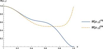
Figure 1. Variation of the sum of two maximum eigenvalues $M{\left({\rho }_{\mathrm{1,2}}\right)}^{{\rm{PB}}}$ and $M{\left({\rho }_{\mathrm{1,2}}\right)}^{{\rm{DM}}}$ with input state α ranging from 0 to 1. |
4.3.2. Non-violation of Bell's inequality of concatenated DMs
For the different values of input states α ∈ (0, 1), the sum of two maximum eigenvalues of concatenated DMs $M{\left({\rho }_{\mathrm{1,2}}\right)}^{{\rm{PB}}* {\rm{DM}}}$ and $M{\left({\rho }_{\mathrm{1,2}}\right)}^{{\rm{DM}}* {\rm{PB}}}$ is the same which is given by
$\begin{eqnarray}M{\left({\rho }_{\mathrm{1,2}}\right)}^{{\rm{PB}}* {\rm{DM}}}=M{\left({\rho }_{\mathrm{1,2}}\right)}^{{\rm{DM}}* {\rm{PB}}}={\left(1-2{\alpha }^{2}\right)}^{2}.\end{eqnarray}$
Using equation (35 ), a comparison graph is plotted between $M{\left({\rho }_{\mathrm{1,2}}\right)}^{{\rm{PB}}* {\rm{DM}}}$ and $M{\left({\rho }_{\mathrm{1,2}}\right)}^{{\rm{DM}}* {\rm{PB}}}$ with input state α as shown in figure 2. It is evident from the graph that the sum of the two maximum eigenvalues of concatenated DMs is less than one. We observe from figure 2 that the output entangled states of concatenated DMs do not violate Bell's inequality. Therefore, the output states generated by one shot and concatenated DMs are entangled but do not violate Bell's inequality.
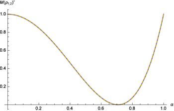
Figure 2. Variation of the sum of two maximum eigenvalues $M{\left({\rho }_{\mathrm{1,2}}\right)}^{{\rm{PB}}* {\rm{DM}}}$ and $M{\left({\rho }_{\mathrm{1,2}}\right)}^{{\rm{DM}}* {\rm{PB}}}$ with input state α ranging from 0 to 1. |
4.4. Teleportation channel
We explore the possibility of using the entangled output state as a teleportation channel. From the knowledge of eigenvalues, we can define the teleportation fidelity as
$\begin{eqnarray}{F}_{\max }=\displaystyle \frac{1}{2}\left(1+\displaystyle \frac{\left(\sqrt{{u}_{1}}+\sqrt{{u}_{2}}+\sqrt{{u}_{3}}\right)}{3}\right),\end{eqnarray}$
where u1, u2, and u3 are the eigenvalues of the matrix U [28]. The output states of the DMs can be used as a teleportation channel if and only if the teleportation fidelity ${F}_{\max }$ is greater than the classical limit of (2/3), i.e, $\begin{eqnarray}{F}_{\max }\gt \displaystyle \frac{2}{3}.\end{eqnarray}$
The teleportation fidelity helps to determine whether the output states of the DMs can act as a teleportation channel.4.4.1. Teleportation fidelity of one shot DMs
First, we analyze the one shot PB and DM. We determine ${F}_{\max }$ for various input parameter values. The teleportation fidelity of the one shot DMs ${F}_{\max }^{{\rm{PB}}}$ and ${F}_{\max }^{{\rm{DM}}}$ are given respectively as
$\begin{eqnarray}\begin{array}{l}{F}_{\max }^{{\rm{PB}}}=\displaystyle \frac{1}{12}\left(6+4\sqrt{{\alpha }^{4}{\left(-1+{\alpha }^{2}\right)}^{2}}\right.\\ \quad +\,2\sqrt{2}\sqrt{1-4{\alpha }^{2}+12{\alpha }^{4}-16{\alpha }^{6}+8{\alpha }^{8}+\left(1-2{\alpha }^{2}\right)\sqrt{1-4{\alpha }^{2}+20{\alpha }^{4}-32{\alpha }^{6}+16{\alpha }^{8}}}).\end{array}\end{eqnarray}$
$\begin{eqnarray}{F}_{\max }^{{\rm{DM}}}=\displaystyle \frac{\left(2+{\alpha }^{2}-{\alpha }^{4}\right)}{3}.\end{eqnarray}$
The expressions given in equations (38 ) and (39 ) are plotted and hence we have figure 3. It is observed from figure 3 that the values of teleportation fidelity of one shot DMs are always greater than the classical limit (2/3) ∀α ∈ (0, 1). Thus, the output states of both one shot DMs can be used as a teleportation channel for all values of inputs. The minimum value of ${F}_{\max }^{{\rm{PB}}}$ and ${F}_{\max }^{{\rm{DM}}}$ is 2/3, when α = 0 or α = 1 corresponding to the input state ∣1⟩ and ∣0⟩, respectively. ${F}_{\max }^{{\rm{PB}}}$ and ${F}_{\max }^{{\rm{DM}}}$ approach the maximum value of 3/4 when $\alpha =\tfrac{1}{\sqrt{2}}$ corresponds to the superposition input state $| \psi \rangle =\tfrac{(| 0\rangle +| 1\rangle )}{\sqrt{2}}$.
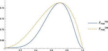
Figure 3. Variation of the teleportation fidelity of one shot DMs ${F}_{\max }^{{\rm{PB}}}$ and ${F}_{\max }^{{\rm{DM}}}$. |
4.4.2. Teleportation fidelity of concatenated DMs
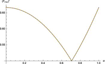
Teleportation fidelity ${F}_{\max }$ is calculated from the eigenvalues of matrix U. It is found that the teleportation fidelities of concatenated DMs ${F}_{\max }^{{\rm{PB}}* {\rm{DM}}}$ and ${F}_{\max }^{{\rm{DM}}* {\rm{PB}}}$ are the same and given by
$\begin{eqnarray}{F}_{\max }^{{\rm{PB}}* {\rm{DM}}}={F}_{\max }^{{\rm{DM}}* {\rm{PB}}}=\displaystyle \frac{1}{6}\left(3+\sqrt{{\left(2{\alpha }^{2}-1\right)}^{2}}\right).\end{eqnarray}$
A graph is plotted between ${F}_{\max }^{{\rm{PB}}* {\rm{DM}}}$ and ${F}_{\max }^{{\rm{DM}}* {\rm{PB}}}$ with input state α as shown in figure 4. We can conclude from figure 4 that the value of teleportation fidelity of a concatenated DM is always less than the classical limit (2/3) ∀α ∈ (0, 1). Therefore, the output of concatenated DMs cannot serve as a teleportation channel. The minimum value of ${F}_{\max }^{{\rm{PB}}* {\rm{DM}}}$ and ${F}_{\max }^{{\rm{DM}}* {\rm{PB}}}$ is 1/2 when $\alpha =\tfrac{1}{\sqrt{2}}$ corresponding to the superposition input state $| \psi \rangle =\tfrac{(| 0\rangle +| 1\rangle )}{\sqrt{2}}$. ${F}_{\max }^{{\rm{PB}}* {\rm{DM}}}$ and ${F}_{\max }^{{\rm{DM}}* {\rm{PB}}}$ approach the maximum value of 2/3, when α = 0 or α = 1 corresponding to the input state ∣1⟩ and ∣0⟩, respectively.
Figure 4. Variation of the teleportation fidelity of concatenated DMs ${F}_{\max }^{{\rm{PB}}* {\rm{DM}}}$ and ${F}_{\max }^{{\rm{DM}}* {\rm{PB}}}$. |
5. Discussion
In this work, we have analyzed one shot DMs, namely the PB and DM. From the analysis of majorization and mixed state, it is found that the output states generated out of one shot DMs are of mixed entangled type. Violation of Bell's inequality is studied as one of the characteristics of the output states of DMs. It is found that the output states of both one shot DMs do not violate Bell's inequalities. Further, teleportation fidelity exceeds the classical limit (2/3) for all input states. Further, the superposition input state achieves maximum teleportation fidelity of 3/4. In short, the output states of both one shot DMs are of mixed entangled type and do not violate Bell's inequality but can be used as a teleportation channel. Therefore, the characteristics of the DMs PB and DM are the same and this is symbolically represented as
$\begin{eqnarray}[{\rm{PB}}]\equiv [{\rm{DM}}].\end{eqnarray}$
We wished to study the effect of changing the order of DMs in the process of concatenation. According to the analysis of majorization and mixed state, we have observed that the output states of concatenated DMs named PB*DM and DM*PB DMs are of the mixed entangled type. We have also shown that the output states of both concatenated DMs do not violate Bell's inequalities. Interestingly, teleportation fidelity does not exceed the classical limit (2/3). Therefore, the output states of both concatenated DMs are of mixed entangled type, do not violate Bell's inequality, and cannot be used as a teleportation channel. Thus, the characteristics of the concatenated DMs PB*DM and DM*PB are the same and represented as
$\begin{eqnarray}\left[{\rm{PB}}\,\ast \,{\rm{DM}}\right]\equiv \left[{\rm{DM}}\,\ast \,{\rm{PB}}\right].\end{eqnarray}$
From the analysis, it is evident that the characteristics of DMs are independent of the order of concatenation. However, generalizing this observation requires detailed investigation. We have compared the characteristics of one shot and concatenated DMs in table 1. It is clear from table 1 that the one shot deletion is useful as it can generate output states that can be used as a teleportation channel. This is not the case with the concatenated DMs. In other words, the output states of concatenated DMs are not useful for acting as a teleportation channel.
Table 1. Comparison of the one shot and concatenated DMs. |
| Deleting | Mixed/pure state | Majorization | Violation of Bell's inequality | Can be a teleportation |
|---|---|---|---|---|
| machines | condition | channel | ||
| PB | Mixed | Inseparable | No | Yes |
| DM | Mixed | Inseparable | No | Yes |
| PB*DM | Mixed | Inseparable | No | No |
| DM*PB | Mixed | Inseparable | No | No |
In our earlier work, we examined the performance of successive deletion of the same DMs [34] to check the possibility of better deletion. In the present work, we have studied the performance of successive deletion of concatenation of different DMs. By combining the results of both works, one can prove that the characteristics of successive deletion satisfy the following associative properties:
| (i) $\mathrm{PB}\,\ast \,\left[{\rm{DM}}\,\ast \,{\rm{PB}}\right]\equiv \left[{\rm{PB}}\,\ast \,{\rm{DM}}\right]\,\ast \,\,\mathrm{PB}$. | |
| (ii) $\mathrm{DM}\,\ast \,\left[{\rm{PB}}\,\ast \,{\rm{DM}}\right]\equiv \left[{\rm{DM}}\,\ast \,{\rm{PB}}\right]\,\ast \,\mathrm{DM}$. |
As a result, we conclude that the characteristics remain unchanged under the successive deletion of different DMs. These findings indicate that we can do the same observation with one shot DMs instead of the successive deletion of different DMs. Hence, we confirm that one shot deletion is said to be more advantageous than successive deletion. Therefore, the results of our work have brought better understanding of the concatenation process, which could be useful in the physical implementation of DMs in the future.