Welcome to visit Communications in Theoretical Physics,
Statistical Physics, Soft Matter and Biophysics

Relativistic transformation of thermodynamic parameters and refined Saha equation

  • Xin Hao , 1 ,
  • Shaofan Liu , 2 ,
  • Liu Zhao , 2, *
Expand
  • 1College of Physics, Hebei Normal University, Shijiazhuang 050024, China
  • 2School of Physics, Nankai University, Tianjin 300071, China

*Author to whom all correspondence should be addressed - change not implemented

Received date: 2022-11-09

  Revised date: 2022-12-26

  Accepted date: 2022-12-27

  Online published: 2023-03-20

Copyright

© 2023 Institute of Theoretical Physics CAS, Chinese Physical Society and IOP Publishing

Abstract

The relativistic transformation rule for temperature is a debated topic for more than 110 years. Several incompatible proposals exist in the literature but a final resolution is still missing. In this work, we reconsider the problem of relativistic transformation rules for a number of thermodynamic parameters including temperature, chemical potential, pressure, entropy and enthalpy densities for a relativistic perfect fluid using relativistic kinetic theory. The analysis is carried out in a fully relativistic covariant manner, and the explicit transformation rules for the above quantities are obtained in both Minkowski and Rindler spacetimes. Our results suggest that the temperature of a moving fluid appears to be colder, supporting the proposal by de Broglie, Einstein, and Planck, in contrast to other proposals. Moreover, in the case of a Rindler fluid, our findings suggest that the total number of particles and the total entropy of a perfect fluid in a box whose bottom is parallel to the Rindler horizon are proportional to the area of the bottom, but are independent of the height of the box, provided the bottom of the box is sufficiently close to the Rindler horizon. The area dependence of the particle number implies that the particles tend to be gathered toward the bottom of the box, and hence implicitly determines the distribution of the chemical potential of the system, whereas the area dependence of the entropy indicates that the entropy is still additive and may have potential applications in explaining the area law of black hole entropy. As a by-product, we also obtain a relativistically refined version of the famous Saha equation which holds in both Minkowski and Rindler spacetimes.

Cite this article

Xin Hao , Shaofan Liu , Liu Zhao . Relativistic transformation of thermodynamic parameters and refined Saha equation[J]. Communications in Theoretical Physics, 2023 , 75(3) : 035601 . DOI: 10.1088/1572-9494/acae81

1. Introduction

Of all branches of modern physics, classical thermodynamics and relativity are outstanding in the sense that they describe the universal rules that every physical system must obey, irrespective of the detailed matter contents of the system. There are only two requirements for classical thermodynamics to hold: (i) the physical system needs to be macroscopic, i.e. containing a large number of microscopic degrees of freedom, (ii) the system needs to be at thermodynamic equilibrium with uniform temperature and pressure. In contrast, there seems to be no requirement for any physical system to obey the principles of relativity, although the special relativistic effects can only become manifest when the system undergoes very fast motion in comparison to the speed of light, and the general relativistic effects can only become manifest when the system contains a huge amount of mass and/or energy.
It has long been fascinating to consider situations when the principles of both classical thermodynamics and relativity apply. Such situations involve a macroscopic system that either undergoes relativistic motion or moves in curved spacetime. Endeavors in combining thermodynamics and relativity have lasted for over 110 years. However, the outcome is quite controversial. Even without considering the general relativistic effects, the combination of classical thermodynamics and special relativity has led to several contradictory results on the transformation rule for temperature. Basically, there are four major views on such transformations, each labeled by the names of the corresponding researchers below (wherein γ > 1 is the Lorentz factor):
i

(i) de Broglie [1], Einstein [2] and Planck [3]: moving bodies appear cooler, $T^{\prime} ={\gamma }^{-1}T;$

ii

(ii) Eddington [4], Ott [5] and Arzelies [6]: moving bodies appear hotter, $T^{\prime} =\gamma T;$

iii

(iii) Landsberg [7, 8]: temperature is a relativistic invariant, $T^{\prime} =T;$

iv

(iv) Cavalleri, Salgarelli [9] and Newburgh [10]: no unique such transformation because thermodynamics are defined only in the rest frame.

Quite notably, Einstein seems to have supported each of the four views in his life [11], and Lansberg turned to the fourth view in his later career [12, 13]. The debates between all these different views remain open [14] and a huge number of papers have been published on the same or related subjects. It is remarkable that the standing point of the fourth view by Cavalleri et al lies in that a system at thermodynamic equilibrium must be static [9, 10] and hence excludes the existence of macroscopic flow which is inherently implied by the global relativistic motion of the system, and that a moving observer in a heat reservoir cannot detect a blackbody spectrum [12, 13], which implies the nonexistence of a uniform temperature. Such reasonings, however, should not be taken to be sufficient justifications for the fourth view, because there are situations beyond thermodynamic equilibrium when one could talk about the temperature, pressure, and entropy, etc., at least locally, of a given macroscopic system, for instance for systems which are not in global but in local equilibrium, or for systems under detailed balance. For such systems, the classical equilibrium thermodynamics do not apply; however, a description using kinetic theory still works well.
Among the existing papers on related subjects (not necessarily considering the temperature transformations), some considerations from the point of view of statistical mechanics or kinetic theory have been introduced. Some authors [15-18] started right from equilibrium statistical mechanics or Gibbs distributions and the formulations were often not presented in an explicitly relativistic covariant fashion, hence not best suited for analyzing the transformation rules for macroscopic parameters. Some other works either dealt with the debates about the correct relativistic distribution function [19, 20] or introduced some modifications to the distribution function [21].
In order to solve the puzzles on the relativistic transformation rules for macroscopic parameters, the necessary statistical mechanics tool needs to be relativistic covariant and applicable to systems out of thermodynamic equilibrium. Such a theory exists and is known as the relativistic kinetic theory. It was established almost immediately after the first view by de Broglie, Einstein and Planck was proposed [22]. Therefore, it is tempting to reconsider the relativistic transformations for macroscopic parameters like temperature and pressure from the point of view of relativistic kinetic theory. As far as we know, a fully covariant treatment for this problem using relativistic kinetic theory has not been reported before in the literature, so we decided to work it out by ourselves.
Before dwelling on the detailed analysis, it is worth pointing out that the aforementioned debates stem largely from the way that the question is raised. All previous works on this subject prescribe the question as follows: Assuming the temperature of a system in (local) thermodynamic equilibrium is T in the rest frame, what is its temperature $T^{\prime} $ in a frame in which the system undergoes fast motion? An alternative prescription of the question which does not rely on the choice of coordinate frames can be given as follows. Assuming the system is at (local) thermodynamic equilibrium at temperature T with respect to the comoving observer, what is its temperature $T^{\prime} $ with respect to a non-comoving observer? The two prescriptions differ from each other in the reason why such changes happen. The first prescription attributes the change of temperature to the change of coordinate frames, while the second prescription attributes the change to the change of observers. Even so, both prescriptions quest the change of the temperature of the system at the same macrostate, and the change of temperature in both prescriptions arises purely from kinematic effects. Therefore, both prescriptions can be dubbed as the kinematic version of the question. There is a dynamic version of the question that quests for the temperature of the system which is initially at rest and then pushed into fast motion. This version breaks the initial macrostate and will not be discussed here.
In this work, we take the second kinematic prescription as the starting point. The reason to take the second rather than the first prescription is due to the following considerations. First of all, most thermodynamic parameters have phenomenological interpretations and their values are naturally observer-dependent. The first kinematic prescription does not provide information about such dependences. Second, we hope to understand the relativistic transformation rules for thermodynamic parameters in more generic spacetimes rather than just in Minkowski spacetime. Therefore, the coordinate changes do not necessarily belong to the set of Lorentz transformations. Last but not least, we show that most of the thermodynamic parameters (or densities thereof) can be defined as scalars with respect to the coordinate transformations, whereas their transformation rules under a change of observers are still nontrivial. This last reasoning indicates that the first prescription is actually ill-posed.
As will be shown in the main context, our analysis indicates that the transformation rule of temperature agrees with the view of de Broglie, Einstein, and Planck, but with the addition of the transformation rules for a number of other thermodynamic parameters, notably including the chemical potential μ, the particle number density n, and the enthalpy density w. Our analysis indicates that the transformation rules of those parameters are identical in both Minkowski and Rindler spacetimes, and we expect that the same rules should also be valid in other backgrounds as well due to the fully relativistic covariant formalism. In the case of the Rindler background, we also show that the total number of particles and the total entropy of a perfect fluid system in a box are proportional to the area of the bottom of the box which is parallel to the Rindler horizon, but are independent of the height of the box, provided the bottom of the box is sufficiently close to the Rindler horizon. Moreover, since the chemical potential is explicitly calculated in our considerations, it is straightforward to obtain a relativistically refined version of the famous Saha equation [23] which characterizes the local chemical equilibrium in the ultra-relativistic regime.

2. Elements of relativistic kinetic theory

Our main tool is relativistic kinetic theory based on a covariant generalization of the Boltzmann equation. This theory is a subfield of non-equilibrium statistical physics, and the application of this theory in our analysis implies some microscopic considerations are involved. In contrast with the Gibbs method for an equilibrium system, in kinetic theory, the distribution function is taken to be the one-particle distribution function (1PDF) f(x, p) which is defined to be the local particle number density in the one-particle phase space. In relativistic settings, one often enlarges the one-particle phase space to the tangent bundle of the full spacetime3(For the sake of generality, we do not require the spacetime to be flat; thus, the formulation of the relativistic kinetic theory to be described below applies to both special and general relativistic cases.), of which the fiber space is spanned by the proper momentum vector pμ for individual particles which obey the mass shell constraint pμpμ = − m2c2, where m is the rest mass of the particle. The enlarged one-particle phase space is endowed with a relativistic invariant measure [24, 25] Ω = ϖε, where ${\boldsymbol{\varpi }}=\tfrac{\sqrt{g}}{| {p}_{0}| }{{\rm{d}}}^{d}p$ is the momentum space volume element4(The appearance of ddp rather than dd+1p is due to the mass shell constraint.), ${\boldsymbol{\epsilon }}=\sqrt{g}{{\rm{d}}}^{d+1}x$ is the spacetime volume element, $g=| \det ({g}_{\mu \nu })| $, and d + 1 is the spacetime dimension. For a dilute gas system, in much of the region in phase space, the 1PDF is locally conserved:
$\begin{eqnarray}{{\mathscr{L}}}_{{ \mathcal H }}f=0,\end{eqnarray}$
where ${{\mathscr{L}}}_{{ \mathcal H }}$ denotes the Lie derivatives along the Hamiltonian vector field ${ \mathcal H }$. This is known as the relativistic Liouville equation. However, taking into account the contribution from the inter-particle scatterings, the Liouville equation should be replaced by the Boltzmann equation
$\begin{eqnarray}{{\mathscr{L}}}_{{ \mathcal H }}f={ \mathcal C }(x,p),\end{eqnarray}$
where the scattering integral ${ \mathcal C }(x,p)$ is a non-local integral in terms of the 1PDF f(x, p) and the local transition rate W(xp1, p2; p3, p4) if two particle scatterings are dominated. Assuming that the above equation is solved, all macroscopic evolutions of the non-equilibrium system are determined by the 1PDF, including the particle number current Nμ, the energy-momentum tensor Tμν, and the entropy current Sμ:
$\begin{eqnarray*}\begin{array}{rcl}{N}^{\mu } & = & c\int {\boldsymbol{\varpi }}{p}^{\mu }f,\qquad {T}^{\mu \nu }=c\int {\boldsymbol{\varpi }}{p}^{\mu }{p}^{\nu }f,\\ {S}^{\mu } & = & -{k}_{{\rm{B}}}c\int {\boldsymbol{\varpi }}{p}^{\mu }f\left[\mathrm{log}({h}^{d}f)-1\right],\end{array}\end{eqnarray*}$
wherein h is the Planck constant and kB is the Boltzmann constant. Since the Boltzmann equation is an integro-differential equation, finding a solution is a highly nontrivial task. Fortunately, we can draw some interesting conclusions without too much effort in solving the equation. As long as the Boltzmann equation holds, the particle number is conserved, ∇μNμ = 0, the hydrodynamic equation is established, ∇μTμν = 0, and the entropy never decreases, ${ \mathcal G }\equiv {{\rm{\nabla }}}_{\mu }{S}^{\mu }\geqslant 0$. ${ \mathcal G }$ is known as the local entropy production rate, and when ${ \mathcal G }=0$, the system is in detailed balance.
Under detailed balance, one can show that $\mathrm{log}({h}^{d}f)$ is additive and must be linearly dependent on additive conserved quantities of the macroscopic system. Meanwhile, the Boltzmann equation degenerates into the Liouville equation (1). With all these conditions we can conclude that the general form of the 1PDF under detailed balance is
$\begin{eqnarray}{f}_{0}=\displaystyle \frac{1}{{h}^{d}}\exp (-\alpha +{{ \mathcal B }}_{\mu }{p}^{\mu }),\end{eqnarray}$
where α and ${{ \mathcal B }}_{\mu }$ are undetermined coefficients which satisfy
$\begin{eqnarray}-{p}^{\mu }{\partial }_{\mu }\alpha +{p}^{\mu }{p}^{\nu }{{\rm{\nabla }}}_{\mu }{{ \mathcal B }}_{\nu }=0.\end{eqnarray}$
We assume that the motion of individual particles is completely random, so the coefficients in front of the linear and quadratic terms in the momentum must separately be zero. Hence we have
$\begin{eqnarray}{\partial }_{\mu }\alpha =0,\qquad \mathrm{and}\qquad {{\rm{\nabla }}}_{(\mu }{{ \mathcal B }}_{\nu )}=0.\end{eqnarray}$
Ignoring the trivial solution ${{ \mathcal B }}^{\mu }=0$, it follows from equation (5) that ${{ \mathcal B }}^{\mu }$ must be a Killing vector field. Let us reiterate that the 1PDF (3) applies to any classical macroscopic system in any spacetime admitting a Killing vector field ${{ \mathcal B }}^{\mu }$, provided the system is under detailed balance. The form of the 1PDF (3) reminds us of the famous Jüttner distribution [22, 26-28]
$\begin{eqnarray}f=\displaystyle \frac{1}{{h}^{d}}\exp (-\alpha +\beta {U}_{\mu }{p}^{\mu }),\end{eqnarray}$
for a relativistic fluid in equilibrium, wherein Uμ is the average proper velocity of the fluid element and β is the inverse temperature. However, at this point, we do not attempt to link ${{ \mathcal B }}_{\mu }$ with Uμ, and do not introduce an a priori inverse temperature. The system described by the 1PDF (3) is only in detailed balance but not in thermodynamic equilibrium. As will be shown later, if we choose an instantaneously comoving observer while describing the motion of the fluid, the distribution (3) indeed reduces to the standard Jüttner distribution (6). However, if we choose an arbitrary non-comoving observer, equation (3) differs from the Jüttner distribution (6), which allows us to uncover the transformation rules for macroscopic quantities.
The solution to equation (5) can be non-unique because the spacetime may admit several independent Killing vector fields. In such cases, ${{ \mathcal B }}^{\mu }$ can be either timelike or spacelike. Accordingly, the quantity ${{ \mathcal B }}_{\mu }{p}^{\mu }$ can be proportional either to the single particle energy or to certain momentum component(s) of the single particle. It is not surprising that the 1PDF can depend on the momentum component(s) of the particle. Even in non-relativistic statistical mechanics, the distribution function can depend on the particle momentum if the system maintains spatial translation symmetry. However, there may be surprising cases if the spacetime has no timelike Killing vector but does have several spacelike ones. In such spacetimes, the detailed balance distribution of the form (3) can still be achieved. This possibility is of little interest if one considers the fact that the macroscopic system needs to be spatially confined by a potential that breaks all spatial translational symmetries. In short, although the solutions to equation (5) depend solely on the spacetime diffeomorphism symmetry, the physical choice of the solution can only be determined by considering the symmetry of the potential as well as the boundary conditions of the system. In the present work, we assume that the spacetime and the boundary conditions of the system altogether admit at least one timelike ${{ \mathcal B }}^{\mu }$. We also assume that ${{ \mathcal B }}^{\mu }$ is normalized as ${{ \mathcal B }}^{2}=-{\beta }^{2}{c}^{2}$, in which the physical meaning of the scalar parameter β is yet to be interpreted. In order to have an intuitive understanding of this parameter, let us temporarily consider a two-component mixture consisting of species (I) and (II) between which only elastic scatterings could occur. For such a system, the detailed balance condition reduces to equation [26],
$\begin{eqnarray*}{f}_{{\rm{I}}}({p}_{{\rm{I}}}){f}_{\mathrm{II}}({p}_{\mathrm{II}})={f}_{{\rm{I}}}^{{\prime} }({p}_{{\rm{I}}}^{{\prime} }){f}_{\mathrm{II}}^{{\prime} }({p}_{\mathrm{II}}^{{\prime} }),\end{eqnarray*}$
where unprimed and primed symbols represent respectively the corresponding quantities before and after the elastic scattering. Accordingly,
$\begin{eqnarray*}{{ \mathcal B }}_{({\rm{I}})\mu }{p}_{({\rm{I}})}{}^{\mu }+{{ \mathcal B }}_{(\mathrm{II})\mu }{p}_{(\mathrm{II})}{}^{\mu }={{ \mathcal B }}_{({\rm{I}})\mu }{p}_{({\rm{I}})}^{{\prime} }{}^{\mu }+{{ \mathcal B }}_{(\mathrm{II})\mu }{p}_{(\mathrm{II})}^{{\prime} }{}^{\mu }\end{eqnarray*}$
is satisfied for any elastic binary collision, ${p}_{({\rm{I}})}{}^{\mu }+{p}_{(\mathrm{II})}{}^{\mu }={p}_{({\rm{I}})}^{{\prime} }{}^{\mu }+{p}_{(\mathrm{II})}^{{\prime} }{}^{\mu }$. Further, with the same boundary conditions, ${{ \mathcal B }}_{({\rm{I}})}^{\mu }$ and ${{ \mathcal B }}_{(\mathrm{II})}^{\mu }$ must be collinear. Therefore β(I) and β(II) must be equal, which means that locally there is a commonly shared scalar for two comoving systems under detailed balance. In this sense, β may be used while defining temperature. This argument agrees in spirit with [19]. Later, we show that β is indeed connected to the inverse temperature observed by comoving observers in more generic settings rather than just in the two-component mixture described above.
Using the detailed balance distribution (3), we can rewrite the particle number current, the energy-momentum tensor, and the entropy current under detailed balance as follows:
$\begin{eqnarray}\begin{array}{rcl}{N}^{\mu } & = & \displaystyle \frac{c\,{{\rm{e}}}^{-\alpha }}{{h}^{d}}\int \displaystyle \frac{\sqrt{g}\,{{\rm{d}}}^{d}p}{| {p}_{0}| }{p}^{\mu }{{\rm{e}}}^{{{ \mathcal B }}_{\rho }{p}^{\rho }},\\ {T}^{\mu \nu } & = & \displaystyle \frac{c\,{{\rm{e}}}^{-\alpha }}{{h}^{d}}\int \displaystyle \frac{\sqrt{g}\,{{\rm{d}}}^{d}p}{| {p}_{0}| }{p}^{\mu }{p}^{\nu }{{\rm{e}}}^{{{ \mathcal B }}_{\rho }{p}^{\rho }},\end{array}\end{eqnarray}$
$\begin{eqnarray}\begin{array}{l}{S}^{\mu }=\displaystyle \frac{{k}_{{\rm{B}}}c\,{{\rm{e}}}^{-\alpha }}{{h}^{d}}\int \displaystyle \frac{\sqrt{g}\,{{\rm{d}}}^{d}p}{| {p}_{0}| }\left(1+\alpha -{{ \mathcal B }}_{\nu }{p}^{\nu }\right){p}^{\mu }{{\rm{e}}}^{{{ \mathcal B }}_{\rho }{p}^{\rho }}\\ \quad ={k}_{{\rm{B}}}\left(1+\alpha \right){N}^{\mu }-{k}_{{\rm{B}}}\,{{ \mathcal B }}_{\nu }{T}^{\mu \nu }.\end{array}\end{eqnarray}$
It is evident that provided the conditions (5) are satisfied, the hydrodynamic equations ∇μNμ = 0, ∇μTμν = 0 and the detailed balance condition ∇μSμ = 0 are explicitly satisfied. Therefore, the macroscopic system is non-dissipative and can be modeled as a perfect fluid. Notice, however, that since Nμ, Tμν, and Sμ are all tensorial objects, the components of these objects depend explicitly on the choices of the spacetime geometry and the coordinate system. According to the principles of relativity, the characteristic properties of the perfect fluid need to be described in a way that is independent of the coordinate choice. This can be done by introducing a number of scalar density parameters. Even so, an explicit specification for the spacetime metric gμν is inevitable. In the next section, we calculate the physical quantities for the perfect fluid in Minkowski spacetime and uncover the relativistic transformation rules for a number of scalar observables of the perfect fluid.

3. Transformation rules in Minkowski spacetime

In this section, we fix the spacetime to be Minkowskian, and for simplicity, we set the spacetime dimension to be 3 + 1, and take the coordinates to be Cartesian. Under such settings, the Killing vector field ${{ \mathcal B }}^{\mu }$ can be taken as ${{ \mathcal B }}^{\mu }=\beta {({\partial }_{t})}^{\mu }=\left(\beta c,0,0,0\right)$, and the particle number current Nμ and the energy-momentum tensor Tμν as given in (7) can be explicitly evaluated to be
$\begin{eqnarray}{N}^{\mu }=\left(\displaystyle \frac{4\pi {{\rm{e}}}^{-\alpha }}{{\lambda }_{C}^{3}\zeta }c\,{K}_{2}(\zeta ),0,0,0\right),\end{eqnarray}$
$\begin{eqnarray}\begin{array}{l}{T}^{\mu \nu }=\displaystyle \frac{4\pi {{\rm{e}}}^{-\alpha }}{{\lambda }_{C}^{3}\zeta }{{mc}}^{2}{K}_{2}(\zeta )\\ \quad \times \left(\begin{array}{cccc}\left[{K}_{3}(\zeta )/{K}_{2}(\zeta )-{\zeta }^{-1}\right] & 0 & 0 & 0\\ 0 & {\zeta }^{-1} & 0 & 0\\ 0 & 0 & {\zeta }^{-1} & 0\\ 0 & 0 & 0 & {\zeta }^{-1}\end{array}\right),\end{array}\end{eqnarray}$
where ${\lambda }_{C}=\tfrac{h}{{mc}}$ is the Compton wavelength of the constituent particles, Kν(ζ) is the modified Bessel function of the second kind, and ζ = βmc2 is a dimensionless parameter. It follows from equation (9) that the particle number current has no spatial component, which reflects the fact that we are working in a comoving coordinate system. The particle number density can be read off from the temporal component of Nμ,
$\begin{eqnarray}\bar{n}=\displaystyle \frac{1}{c}{N}^{0}=\displaystyle \frac{4\pi {{\rm{e}}}^{-\alpha }}{{\lambda }_{C}^{3}\zeta }{K}_{2}(\zeta ).\end{eqnarray}$
The energy density is the 00 component of the energy momentum tensor which reads
$\begin{eqnarray}\bar{\epsilon }={T}^{00}=\displaystyle \frac{4\pi {{\rm{e}}}^{-\alpha }}{{\lambda }_{C}^{3}\zeta }{{mc}}^{2}\left[{K}_{3}(\zeta )-{\zeta }^{-1}{K}_{2}(\zeta )\right].\end{eqnarray}$
Moreover, from equation (10), one can see that the stress tensor (regarded as the spatial-spatial part of the energy-momentum tensor) is diagonal, ${\bar{{ \mathcal S }}}^{{ij}}=\bar{P}{\delta }^{{ij}}$, which means that the perfect fluid is characterized by an isotropic pressure
$\begin{eqnarray}\bar{P}={\bar{T}}^{{ii}}=\displaystyle \frac{4\pi {{\rm{e}}}^{-\alpha }}{{\lambda }_{C}^{3}{\zeta }^{2}}{{mc}}^{2}{K}_{2}(\zeta )={\zeta }^{-1}{{mc}}^{2}\bar{n}=\displaystyle \frac{\bar{n}}{\beta }.\end{eqnarray}$
The particle number density $\bar{n}$, the pressure $\bar{P}$ and the energy density $\bar{\epsilon }$ given above are taken to be some specific component (or sum of components) of the relevant tensors. This may raise concerns about the relativistic invariance (or covariance) of these quantities. However, the fact is that there is an observer, say $\bar{{ \mathcal O }}$, hidden in the above result. To be specific, at each given spacetime event, the proper velocity of $\bar{{ \mathcal O }}$ is ${\bar{Z}}^{\mu }={({\partial }_{t})}^{\mu }$, and $\bar{n}$ and $\bar{\epsilon }$ are actually the following scalar observables measured by the observer $\bar{{ \mathcal O }}$,
$\begin{eqnarray}\bar{n}=-\displaystyle \frac{1}{{c}^{2}}{\bar{Z}}_{\mu }{N}^{\mu },\qquad \bar{\epsilon }=\displaystyle \frac{1}{{c}^{2}}{\bar{Z}}_{\mu }{\bar{Z}}_{\nu }{T}^{\mu \nu },\end{eqnarray}$
and the pressure $\bar{P}$ is simply one third of the trace of the pure stress tensor ${\bar{{ \mathcal S }}}^{\mu \nu }$ (now regarded as a tensor on the full spacetime) measured by $\bar{{ \mathcal O }}$:
$\begin{eqnarray}{\bar{{ \mathcal S }}}^{\mu \nu }\equiv {T}^{\rho \sigma }{\bar{{\rm{\Delta }}}}_{\rho }{}^{\mu }{\bar{{\rm{\Delta }}}}_{\sigma }{}^{\nu },\qquad \bar{P}=\displaystyle \frac{1}{3}{\bar{{\rm{\Delta }}}}_{\mu \nu }{\bar{{ \mathcal S }}}^{\mu \nu },\end{eqnarray}$
where
$\begin{eqnarray*}{\bar{{\rm{\Delta }}}}^{\mu \nu }={\eta }^{\mu \nu }+\displaystyle \frac{1}{{c}^{2}}{\bar{Z}}^{\mu }{\bar{Z}}^{\nu }\end{eqnarray*}$
is the normal projection tensor associated to the observer $\bar{{ \mathcal O }}$ which satisfies
$\begin{eqnarray*}\begin{array}{l}{\bar{{\rm{\Delta }}}}_{\mu \nu }{\bar{Z}}^{\mu }=0,\quad {\bar{{\rm{\Delta }}}}_{\mu \nu }{v}^{\mu }={v}^{\nu },\\ \quad \forall {v}^{\mu }\,{\rm{such}}\,{\rm{that}}\,{\bar{Z}}_{\mu }{v}^{\mu }=0.\end{array}\end{eqnarray*}$
${\bar{{\rm{\Delta }}}}_{\mu \nu }$ is also the induced metric on the spacelike hypersurface normal to ${\bar{Z}}^{\mu }$. From the above point of view, $\bar{n}$, $\bar{\epsilon }$ and $\bar{P}$ are all scalar observables that are independent of coordinate choices, but dependent on the choice of observer.
In a static spacetime, an observer whose proper velocity is proportional to ${({\partial }_{t})}^{\mu }$ is known as a static observer. The choice of the static observer $\bar{{ \mathcal O }}$ leads to the following consequences: (i) ${{ \mathcal B }}^{\mu }$ and ${\bar{Z}}^{\mu }$ are collinear, ${{ \mathcal B }}^{\mu }=\beta {\bar{Z}}^{\mu };$ (ii) Nμ has no spatial components with respect to ${\bar{Z}}^{\mu }$, i.e. ${N}^{\mu }{\bar{{\rm{\Delta }}}}_{\mu }{}^{\nu }=0;$ (iii) the stress measured by $\bar{O}$ is isotropic. The observer $\bar{{ \mathcal O }}$ is actually an instantaneous comoving observer, which means that the proper velocity of the observer is identical to that of the fluid element. Indeed, according to equations (9) and (10), the particle number current Nμ and energy-momentum tensor Tμν can be expressed in terms of ${\bar{Z}}^{\mu }$ as
$\begin{eqnarray}{N}^{\mu }=\bar{n}{\bar{Z}}^{\mu },\qquad {T}^{\mu \nu }=\bar{P}{\eta }^{\mu \nu }+\displaystyle \frac{1}{{c}^{2}}\left(\bar{\epsilon }+\bar{P}\right){\bar{Z}}^{\mu }{\bar{Z}}^{\nu },\end{eqnarray}$
which recovers the familiar result of the particle number current and energy-momentum tensor for a perfect fluid.
The parametrization of the particle number current and energy-momentum tensor using energy density and pressure is not the only choice. There exist other sets of variables that fulfill the same purposes, some of which may even be more preferable in some cases. For instance, when relativistic transformations are concerned, it may be more reasonable to decompose the above tensorial objects into irreducible parts which do not mix up under local Lorentz boosts. For Tμν, one such decomposition is given as follows:
$\begin{eqnarray*}\begin{array}{rcl}{T}^{\mu \nu } & = & \displaystyle \frac{1}{4}{ \mathcal T }{\eta }^{\mu \nu }+\displaystyle \frac{1}{4}\bar{w}\left({\bar{{\rm{\Delta }}}}^{\mu \nu }+\displaystyle \frac{3}{{c}^{2}}{\bar{Z}}^{\mu }{\bar{Z}}^{\nu }\right),\\ { \mathcal T } & \equiv & {T}^{\sigma }{}_{\sigma }=-\displaystyle \frac{4\pi {{\rm{e}}}^{-\alpha }}{{\lambda }_{C}^{3}\zeta }{{mc}}^{2}{K}_{1}(\zeta ),\\ \bar{w} & \equiv & \bar{\epsilon }+P=\displaystyle \frac{4\pi {{\rm{e}}}^{-\alpha }}{{\lambda }_{C}^{3}\zeta }{{mc}}^{2}{K}_{3}(\zeta ),\end{array}\end{eqnarray*}$
where ${ \mathcal T }$ is the trace of Tμν and $\bar{w}$ represents the enthalpy density. The decomposition of Tμν now consists of its trace and traceless parts. Generally speaking, the trace part satisfies5(Our convention on the metric signature is (−, + , + , + ).)${ \mathcal T }\leqslant 0$, and the enthalpy density satisfies $\bar{w}\geqslant 0$. Now we proceed to study the entropy density. By use of equation (16), the entropy current (8) becomes
$\begin{eqnarray}{S}^{\mu }=\bar{s}{\bar{Z}}^{\mu },\qquad \bar{s}={k}_{{\rm{B}}}\left(\beta \,\bar{w}+\bar{n}\alpha \right).\end{eqnarray}$
Now we are in a position to analyze the particle number density n, enthalpy density w, and entropy density s measured by an arbitrary instantaneous observer ${ \mathcal O }$ with proper velocity Zμ. Of course, Zμ should still be a normalized timelike vector at each instance. The normal projection tensor associated with the observer ${ \mathcal O }$ is naturally defined as
$\begin{eqnarray*}{{\rm{\Delta }}}^{\mu \nu }={\eta }^{\mu \nu }+\displaystyle \frac{1}{{c}^{2}}{Z}^{\mu }{Z}^{\nu }.\end{eqnarray*}$
Let us recall that, at the same spacetime event, any two instantaneous observers can be connected by a (local) Lorentz boost. To prove this statement, let us assume that ${\bar{Z}}^{\mu }$ and Zμ are not proportional to each other. Otherwise, the two observers must be identical. At the same event, we can always write
$\begin{eqnarray}{\bar{Z}}^{\mu }=\gamma \left({Z}^{\mu }+{z}^{\mu }\right),\quad \mathrm{where}\quad {Z}_{\mu }{z}^{\mu }=0.\end{eqnarray}$
Clearly, since zμ is normal to Zμ, one has
$\begin{eqnarray*}{{\rm{\Delta }}}_{\mu \nu }{Z}^{\mu }=0,\qquad {{\rm{\Delta }}}_{\mu \nu }{z}^{\mu }={z}_{\nu }.\end{eqnarray*}$
From the normalization condition for ${\bar{Z}}^{\mu }$ and Zμ, it is easy to see that
$\begin{eqnarray*}\gamma =\displaystyle \frac{1}{\sqrt{1-{z}^{2}/{c}^{2}}},\end{eqnarray*}$
so γ is nothing but the Lorentz factor and zμ can be regarded as the relative coordinate time velocity between the two observers $\bar{{ \mathcal O }}$ and ${ \mathcal O }$ (notice that in a coordinate system in which the observer ${ \mathcal O }$ remains static, zμ has no temporal component and thus can be considered as a 3-vector). Notice that although the proper velocity of the observer has been changed, the Killing vector field ${{ \mathcal B }}^{\mu }$ appearing in the distribution function (3) remains untouched. Therefore, ${{ \mathcal B }}^{\mu }$ is not parallel to the proper velocity Zμ of the new observer ${ \mathcal O }$.
Inserting equation (18) into the expressions for Nμ, Tμν (16), and Sμ (17), we get
$\begin{eqnarray}\begin{array}{rcl}{N}^{\mu } & = & \gamma \bar{n}{Z}^{\mu }+\gamma \bar{n}{z}^{\mu },\\ {T}^{\mu \nu } & = & \bar{P}{\eta }^{\mu \nu }+\displaystyle \frac{{\gamma }^{2}}{{c}^{2}}\bar{w}\left[{Z}^{\mu }{Z}^{\nu }+\left({Z}^{\mu }{z}^{\nu }+{Z}^{\nu }{z}^{\mu }\right)+{z}^{\mu }{z}^{\nu }\right],\\ {S}^{\mu } & = & \gamma \bar{s}{Z}^{\mu }+\gamma \bar{s}{z}^{\mu }.\end{array}\end{eqnarray}$
By definition, the particle number density measured by the observer ${ \mathcal O }$ is
$\begin{eqnarray}n=-\displaystyle \frac{1}{{c}^{2}}{Z}_{\mu }{N}^{\mu }=\gamma \bar{n},\end{eqnarray}$
which makes perfect sense in terms of the length contraction effect and considering that on the classical level, the total number of particles in the system is invariant. Similarly, the transformation for entropy density is
$\begin{eqnarray}s=-\displaystyle \frac{1}{{c}^{2}}{Z}_{\mu }{S}^{\mu }=\gamma \bar{s},\end{eqnarray}$
where again the γ factor can be attributed to the length contraction effect. In summary, we can conclude that the total entropy should be invariant under Lorentz boost after a volume integration.
The definition for the pressure P observed by the observer ${ \mathcal O }$ contains some subtleties. We need first to separate the energy momentum 4-vector ${{ \mathcal P }}^{\mu }$ and the pure stress tensor ${{ \mathcal S }}^{\mu \nu }$ from the energy-momentum tensor (19):
$\begin{eqnarray}{{ \mathcal P }}^{\mu }\equiv -\displaystyle \frac{1}{{c}^{2}}{Z}_{\rho }{T}^{\rho \nu }{{\rm{\Delta }}}_{\nu }{}^{\mu }=\displaystyle \frac{{\gamma }^{2}\bar{w}}{{c}^{2}}{z}^{\mu },\end{eqnarray}$
$\begin{eqnarray}{{ \mathcal S }}^{\mu \nu }\equiv {T}^{\rho \sigma }{{\rm{\Delta }}}_{\rho }{}^{\mu }{{\rm{\Delta }}}_{\sigma }{}^{\nu }=\bar{P}{{\rm{\Delta }}}^{\mu \nu }+\displaystyle \frac{{\gamma }^{2}\bar{w}}{{c}^{2}}{z}^{\mu }{z}^{\nu }.\end{eqnarray}$
The existence of a spacelike momentum ${{ \mathcal P }}^{\mu }$ reflects the fact that the observer ${ \mathcal O }$ is not comoving with the fluid. In other words, ${{ \mathcal P }}^{\mu }$ is purely a kinematic effect. Notice also that the second term in the expression for ${{ \mathcal S }}^{\mu \nu }$, i.e.
$\begin{eqnarray*}{\tilde{{ \mathcal S }}}^{\mu \nu }\equiv \displaystyle \frac{{\gamma }^{2}\bar{w}}{{c}^{2}}{z}^{\mu }{z}^{\nu }={{ \mathcal P }}^{\mu }{z}^{\nu },\end{eqnarray*}$
is nothing but the kinematic momentum flow, and hence is also purely kinematically originated, so it may be best referred to as a kinematic stress tensor. This part of the total stress tensor introduces an anisotropy in the diagonal part, yielding different pressures in different spatial directions. However, since the thermodynamic effects have nothing to do with the global kinematics of the fluid, it is better to define the thermodynamic pressure as the trace of the difference between the total stress and the kinematic stress divided by the dimension of the space. In the present case, we have
$\begin{eqnarray}P=\displaystyle \frac{1}{3}{{\rm{\Delta }}}_{\mu \nu }({{ \mathcal S }}^{\mu \nu }-{\tilde{{ \mathcal S }}}^{\mu \nu })=\bar{P},\end{eqnarray}$
which indicates that the thermodynamic pressure is a relativistic invariant.
The definition of pressure is essential to determine the correct enthalpy density, and therefore settles the transformation rules connecting thermodynamic parameters measured by the arbitrary observer ${ \mathcal O }$ and comoving observer $\bar{{ \mathcal O }}$. For enthalpy density, equation (19) and the invariance of pressure (24) imply
$\begin{eqnarray}w\equiv \displaystyle \frac{1}{{c}^{2}}{Z}_{\mu }{Z}_{\nu }{T}^{\mu \nu }+P,\qquad \quad w={\gamma }^{2}\bar{w}.\end{eqnarray}$
In view of the explicit expressions for particle density, entropy density, pressure, and enthalpy density, we find that the local equilibrium state for an arbitrary observer can be parametrized by α, β, and γ. It is important to emphasize that the thermodynamic pressure P(α, β) is isotropic and observer-independent, and its derivative yields the following relations:
$\begin{eqnarray*}\begin{array}{rcl}n & = & -\gamma \beta \displaystyle \frac{\partial P}{\partial \alpha },\quad w=-{\gamma }^{2}\beta \displaystyle \frac{\partial P}{\partial \beta },\\ s & = & -\gamma {k}_{{\rm{B}}}\beta \left(\beta \displaystyle \frac{\partial P}{\partial \beta }+\alpha \displaystyle \frac{\partial P}{\partial \alpha }\right).\end{array}\end{eqnarray*}$
Therefore, the total derivative of P(α, β) yields
$\begin{eqnarray}-{\gamma }^{-1}s{\rm{d}}\left(\displaystyle \frac{1}{{k}_{{\rm{B}}}\beta }\right)+{\rm{d}}P+{\gamma }^{-1}n{\rm{d}}\left(\displaystyle \frac{\alpha }{\beta }\right)=0,\end{eqnarray}$
for a comoving observer, i.e. when γ = 1, this equation is reminiscent of the local version of the Gibbs-Duhem relation, provided the parameters β and α are respectively connected with the inverse temperature and the chemical potential appropriately. In fact, such a reminiscence is true, because a system under detailed balance can be considered to be in local thermodynamic equilibrium, and hence we can use the local Gibbs-Duhem relation to identify the local temperature and chemical potential as
$\begin{eqnarray}\bar{T}=\displaystyle \frac{1}{{k}_{{\rm{B}}}\beta },\qquad \bar{\mu }=-\displaystyle \frac{\alpha }{\beta }.\end{eqnarray}$
According to the basic principles of relativity, the choice of observers should not affect physical identities obeyed by physical observables, although the value of each observable may be affected by different choices. Among the thermodynamic relations, in the light of the standpoint of Israel's theory [29], we now make our fundamental assumption that the local Gibbs-Duhem relation is invariant for different observers. In the present context, equation (26) for different observers should correspond to the same physical identity. In other words, (26) should be the invariant Gibbs-Duhem relation. The direct consequences of the invariance of the Gibbs-Duhem relation are the transformation rules of temperature and chemical potential:
$\begin{eqnarray}T={\gamma }^{-1}\displaystyle \frac{1}{{k}_{{\rm{B}}}\beta }={\gamma }^{-1}\bar{T},\qquad \mu =-{\gamma }^{-1}\displaystyle \frac{\alpha }{\beta }={\gamma }^{-1}\bar{\mu }.\end{eqnarray}$
It should be mentioned that, although the temperature transformation given above has already been suggested by de Broglie, Einstein and Planck, the one for chemical potential is, to the best of our knowledge, a new result. Finally, from equations (20), (21), (25), (28) and the conventional definitions for the Gibbs free energy and Helmholtz free energy, we find that the transformation rules for the densities of all thermodynamic potentials can be expressed in a heuristic unified form, $\varphi =\bar{\varphi }+{z}_{\mu }{{ \mathcal P }}^{\mu }$.
Let us conclude this section by adding two extra remarks.

In relativistic physics, the spacetime dimension is often treated as an adjustable parameter. Whenever one draws some conclusion in relativistic physics, it is necessary to check whether the conclusion holds in generic spacetime dimensions or in some specific dimension. On the other hand, the behaviors of thermodynamic quantities are very sensitive to the dimension of the underlying space. Therefore, it makes sense to check whether the transformation rules uncovered in the present section are specific to (3 + 1)-dimensional Minkowski spacetime or whether they hold in arbitrary spacetime dimensions. In order to answer this question, it is necessary to extend the formulation to an arbitrary spacetime dimension $(d+1)$. In this regard, it is important to note that the fluid configuration is completely determined by $\left(\alpha ,{{ \mathcal B }}^{\mu },n,w,{ \mathcal T }\right)$, wherein, for a perfect fluid, α is a constant, ${{ \mathcal B }}^{\mu }$ is a Killing vector field, and, in Minkowskian backgrounds (see Appendix),

$\begin{eqnarray*}\begin{array}{rcl}n & = & \gamma \left[\displaystyle \frac{2\,{{\rm{e}}}^{-\alpha }}{{\lambda }_{C}^{d}}{\left(\displaystyle \frac{2\pi }{\zeta }\right)}^{\tfrac{d-1}{2}}\right]{K}_{\tfrac{d+1}{2}}(\zeta )=\gamma \bar{n},\\ w & = & {\gamma }^{2}{{mc}}^{2}\left[\displaystyle \frac{2\,{{\rm{e}}}^{-\alpha }}{{\lambda }_{C}^{d}}{\left(\displaystyle \frac{2\pi }{\zeta }\right)}^{\tfrac{d-1}{2}}\right]{K}_{\tfrac{d+3}{2}}(\zeta )={\gamma }^{2}\bar{w},\\ { \mathcal T } & = & -{{mc}}^{2}\left[\displaystyle \frac{2\,{{\rm{e}}}^{-\alpha }}{{\lambda }_{C}^{d}}{\left(\displaystyle \frac{2\pi }{\zeta }\right)}^{\tfrac{d-1}{2}}\right]{K}_{\tfrac{d-1}{2}}(\zeta ).\end{array}\end{eqnarray*}$
The exact results for the particle number density, the enthalpy density, and the trace of the energy-momentum tensor for a perfect relativistic fluid in arbitrary spacetime dimensions, to our knowledge, have not been reported before in the literature. Using these results, it will not be difficult to check that all the transformation rules obtained in the present section are independent of the spacetime dimension.

The temperature, chemical potential, particle number density, entropy and enthalpy densities, and pressure of the perfect fluid are all defined as observer-dependent scalars (or scalar densities). Their transformation rules arise purely from the different choices of observers and have nothing to do with the coordinate choices. It is not surprising that at the same spacetime event, any two instantaneous observers can differ from each other at most by a local Lorentz boost (which is not a coordinate transformation of the spacetime). Such differences are independent of the choice of spacetime geometry. Therefore, it is highly expected that the same transformation rules should hold in other spacetimes, and we shall verify this expectation in Rindler spacetime in the next section.

4. Perfect Rindler fluid and the area law of entropy

The 1PDF under detailed balance given in equation (3) is valid not only in Minkowski spacetime but also in any spacetime admitting a Killing vector field ${{ \mathcal B }}_{\mu }$. In order to show the influence of spacetime geometry on the description of a perfect fluid, let us move on to another familiar spacetime, i.e. the Rindler spacetime with the line element
$\begin{eqnarray}\begin{array}{rcl}{\rm{d}}{s}^{2} & = & {g}_{\mu \nu }{\rm{d}}{x}^{\mu }{\rm{d}}{x}^{\nu }=-{\left(1+\displaystyle \frac{\kappa x}{{c}^{2}}\right)}^{2}{c}^{2}{\rm{d}}{t}^{2}\\ & & +{\rm{d}}{x}^{2}+{\rm{d}}{y}^{2}+{\rm{d}}{z}^{2}.\end{array}\end{eqnarray}$
The coordinates used in writing the line element (29) are henceforth referred to as Rindler coordinates. As is well known, the Rindler spacetime contains an accelerating horizon which is located at xh = − c2κ−1 in the Rindler coordinate system. In this spacetime, the static observer $\bar{{ \mathcal O }}$ has proper velocity ${\bar{Z}}^{\mu }={\left(1+\tfrac{\kappa x}{{c}^{2}}\right)}^{-1}{({\partial }_{t})}^{\mu }$, which is timelike but non-Killing. The timelike Killing vector field ${{ \mathcal B }}^{\mu }$ appearing in the 1PDF (3) normalized as ${{ \mathcal B }}^{2}=-{\beta }^{2}{c}^{2}$ must be proportional to ${\bar{Z}}^{\mu }$, i.e. ${{ \mathcal B }}^{\mu }=\beta {\bar{Z}}^{\mu }=\beta {\left(1+\tfrac{\kappa x}{{c}^{2}}\right)}^{-1}{({\partial }_{t})}^{\mu }$, which, together with the fact that ${\bar{Z}}^{\mu }$ is non-Killing, implies that β must not be constant; rather, it has an explicit x-dependence,
$\begin{eqnarray}\beta (x)=-{\beta }_{0}(x-{x}_{h})/{x}_{h},\end{eqnarray}$
where β0 is a constant equal to the value of β at x = 0. Demanding that β0 has a finite value yields that β becomes very small as the system gets very close to the Rindler horizon. On the other hand, if β(x) approaches a finite nonvanishing value as xxh, then β0 could be infinitely large.
With the above choices of spacetime metric and Killing vector field ${{ \mathcal B }}^{\mu }$, the particle number current Nμ and the energy momentum tensor Tμν can be explicitly calculated using equation (7), yielding
$\begin{eqnarray}{N}^{\mu }=\left[c{\left(1+\displaystyle \frac{\kappa x}{{c}^{2}}\right)}^{-1}\displaystyle \frac{4\pi {{\rm{e}}}^{-\alpha }}{{\lambda }_{C}^{3}\zeta }{K}_{2}(\zeta ),0,0,0\right],\end{eqnarray}$
$\begin{eqnarray}\begin{array}{l}{T}^{\mu \nu }=\displaystyle \frac{4\pi {{\rm{e}}}^{-\alpha }}{{\lambda }_{C}^{3}\zeta }{{mc}}^{2}{K}_{2}(\zeta )\\ \quad \times \left(\begin{array}{cccc}\tfrac{\zeta {K}_{3}(\zeta )-{K}_{2}(\zeta )}{{\left(1+\tfrac{\kappa x}{{c}^{2}}\right)}^{2}\zeta {K}_{2}(\zeta )} & 0 & 0 & 0\\ 0 & {\zeta }^{-1} & 0 & 0\\ 0 & 0 & {\zeta }^{-1} & 0\\ 0 & 0 & 0 & {\zeta }^{-1}\end{array}\right),\end{array}\end{eqnarray}$
where ζ is still defined as ζ = βmc2 and hence is non-constant.
Unlike the case of Minkowski spacetime, now we should not expect to read off the particle number density $\bar{n}$, the energy density $\bar{\epsilon }$ and the pressure $\bar{P}$ directly from the appropriate components of Nμ and Tμν respectively as we did in equations (11), (13) and (12). Rather, we should think of these objects as scalar densities defined in equations (14) and (15). Without much effort it can be shown that $\bar{n}$, $\bar{\epsilon }$ and $\bar{P}$ for the Rindler fluid are given respectively by the following expressions:
$\begin{eqnarray}\bar{n}=-\displaystyle \frac{1}{{c}^{2}}{\bar{Z}}_{\mu }{N}^{\mu }=\displaystyle \frac{4\pi {{\rm{e}}}^{-\alpha }}{{\lambda }_{C}^{3}\zeta }{K}_{2}(\zeta ),\end{eqnarray}$
$\begin{eqnarray}\begin{array}{rcl}\bar{\epsilon } & = & \displaystyle \frac{1}{{c}^{2}}{\bar{Z}}_{\mu }{\bar{Z}}_{\nu }{T}^{\mu \nu }=\displaystyle \frac{4\pi {{\rm{e}}}^{-\alpha }}{{\lambda }_{C}^{3}\zeta }{{mc}}^{2}\\ & & \times \left[{K}_{3}(\zeta )-{\zeta }^{-1}{K}_{2}(\zeta )\right],\end{array}\end{eqnarray}$
$\begin{eqnarray}\bar{P}=\displaystyle \frac{1}{3}{\bar{{\rm{\Delta }}}}_{\mu \nu }{\bar{{ \mathcal S }}}^{\mu \nu }=\displaystyle \frac{4\pi {{\rm{e}}}^{-\alpha }}{{\lambda }_{C}^{3}{\zeta }^{2}}{{mc}}^{2}{K}_{2}(\zeta )=\displaystyle \frac{\bar{n}}{\beta },\end{eqnarray}$
and the decomposition like (16) for Nμ and Tμν still holds, while the only difference comes from the different choice of spacetime metric:
$\begin{eqnarray}\begin{array}{rcl}{N}^{\mu } & = & \bar{n}{\bar{Z}}^{\mu },\\ {T}^{\mu \nu } & = & \bar{P}{g}^{\mu \nu }+\displaystyle \frac{1}{{c}^{2}}\left(\bar{\epsilon }+\bar{P}\right){\bar{Z}}^{\mu }{\bar{Z}}^{\nu }.\end{array}\end{eqnarray}$
These results indicate that the static observer $\bar{{ \mathcal O }}$ is instantaneously comoving with the fluid. Moreover, the entropy density $\bar{s}$ can be evaluated explicitly:
$\begin{eqnarray}\begin{array}{rcl}\bar{s} & = & -\displaystyle \frac{1}{{c}^{2}}{\bar{Z}}_{\mu }{S}^{\mu }=-\displaystyle \frac{{k}_{{\rm{B}}}}{{c}^{2}}{\bar{Z}}_{\mu }\left[\left(1+\alpha \right){N}^{\mu }-{{ \mathcal B }}_{\nu }{T}^{\mu \nu }\right]\\ & = & {k}_{{\rm{B}}}\displaystyle \frac{4\pi {{\rm{e}}}^{-\alpha }}{{\lambda }_{C}^{3}}\left[{K}_{3}(\zeta )+\alpha \displaystyle \frac{{K}_{2}(\zeta )}{\zeta }\right]\\ & = & {k}_{{\rm{B}}}\left(\beta \,\bar{w}+\bar{n}\alpha \right).\end{array}\end{eqnarray}$
All the results given in equations (33)-(37) are in perfect agreement with their Minkowski analogs, as shown in equations (11)-(13), (16) and (17). If we proceed to an arbitrary Rindler observer, the same transformation rules for T, μ, P, s, and w are recovered, with the same interpretations for the parameters α, β. The x dependence of β is then attributed to the Tolman-Ehrenfest effect in Rindler spacetime. We will not bother with details on the transformation rules in Rindler spacetime but only mention that, in this case, the relation (18) between the proper velocities of different observers results in a position-dependent boost factor γ, because now z2 = gμνzμzν is position dependent. Such boosts must be considered to be performed in the tangent space of the spacetime at each event, and are known as local Lorentz boosts.
One thing to be noted, however, is that all the transformation rules mentioned above reflect only the behaviors of the corresponding quantities measured at the same spacetime event by different observers. If one wishes to compare the same quantities at different spacetime events or add up some of the local densities to get the corresponding total quantities, things become drastically different between the Minkowski and Rindler cases. For the Minkowski case, nothing special needs to be taken care of, because the inverse temperature β is a constant, and all the local densities are uniform. For the Rindler case, however, the first thing to be noted is the non-constancy of the inverse temperature β. At different spatial locations with x coordinates x1 and x2, one has
$\begin{eqnarray*}\displaystyle \frac{{\zeta }_{1}}{{\zeta }_{2}}=\displaystyle \frac{{\beta }_{1}}{{\beta }_{2}}=\displaystyle \frac{{x}_{1}-{x}_{h}}{{x}_{2}-{x}_{h}}.\end{eqnarray*}$
This is the well-known Tolman-Ehrenfest effect [30] and it implies that the local densities (33), (34), (37) as well as the pressure (35) in Rindler spacetime are all non-uniform. Due to the constancy of the parameter α, the chemical potential $\bar{\mu }$ in Rindler spacetime is also non-uniform.
Now let us consider a box of gas, of which the height and the bottom area are respectively L and A, and orient the box such that the bottom is parallel to the horizon. Let the coordinate distance of the bottom of the box to the horizon be δ. The relativistic coldness at the bottom of the box is denoted by ζbot, so at any height within the box, we have ζ = (xxh)ζbot/δ, and at the top of the box we have ζtop = (L + δ)ζbot/δ.
The total number of particles and the total entropy in the box can be calculated by a direct spatial volume integration of (33) and (37), yielding
$\begin{eqnarray*}\begin{array}{rcl}\bar{N} & = & A{\int }_{{x}_{h}+\delta }^{{x}_{h}+\delta +L}\bar{n}(x){\rm{d}}x=A\displaystyle \frac{4\pi {{\rm{e}}}^{-\alpha }}{{\lambda }_{C}^{3}}\displaystyle \frac{\delta }{{\zeta }_{\mathrm{bot}}}\\ & & \times \left[\displaystyle \frac{{K}_{1}({\zeta }_{\mathrm{bot}})}{{\zeta }_{\mathrm{bot}}}-\displaystyle \frac{{K}_{1}({\zeta }_{\mathrm{top}})}{{\zeta }_{\mathrm{top}}}\right],\\ \bar{S} & = & A{\int }_{{x}_{h}+\delta }^{{x}_{h}+\delta +L}\bar{s}(x){\rm{d}}x\,=\,A\displaystyle \frac{4\pi {k}_{{\rm{B}}}{{\rm{e}}}^{-\alpha }}{{\lambda }_{C}^{3}}\displaystyle \frac{\delta }{{\zeta }_{\mathrm{bot}}}\\ & & \times \left[{K}_{2}({\zeta }_{\mathrm{bot}})-{K}_{2}({\zeta }_{\mathrm{top}})\right]+(\alpha +2){k}_{{\rm{B}}}\bar{N}.\end{array}\end{eqnarray*}$
When the bottom of the box is very close to the horizon, e.g. δL, the coldness at the bottom and top of the box behave as ζbotζtop. Recalling that both K1(ζ) and K2(ζ) are monotonically decreasing functions, we have K1(ζbot) ≫ K1(ζtop), K2(ζbot) ≫ K2(ζtop). Then from equation (33) one finds that the particles tend to be gathered at the bottom of the box, and the total number of particles and entropy can be approximated as
$\begin{eqnarray*}\begin{array}{rcl}\bar{N} & \approx & A\displaystyle \frac{4\pi {{\rm{e}}}^{-\alpha }}{{\lambda }_{C}^{3}}\displaystyle \frac{\delta }{{\zeta }_{\mathrm{bot}}^{2}}{K}_{1}({\zeta }_{\mathrm{bot}}),\\ \bar{S} & \approx & A\displaystyle \frac{4\pi {k}_{{\rm{B}}}{{\rm{e}}}^{-\alpha }}{{\lambda }_{C}^{3}}\displaystyle \frac{\delta }{{\zeta }_{\mathrm{bot}}^{2}}\left[(\alpha +2){K}_{1}({\zeta }_{\mathrm{bot}})\right.\\ & & \left.+{\zeta }_{\mathrm{bot}}{K}_{2}({\zeta }_{\mathrm{bot}})\right],\end{array}\end{eqnarray*}$
which are both independent of the height of the box and proportional to the area of the bottom of the box. These results are similar to those in [15-17] where the particle number and entropy are obtained through completely different approaches. For closed classical systems, the number of particles needs to be constant, and the expression for $\bar{N}$ actually determines the chemical potential distribution implicitly. Comparing the values of $\bar{N}$ and $\bar{S}$ in the above case, we get
$\begin{eqnarray}\bar{S}\approx \bar{N}{k}_{{\rm{B}}}\left[(\alpha +2)+\displaystyle \frac{{\zeta }_{\mathrm{bot}}{K}_{2}({\zeta }_{\mathrm{bot}})}{{K}_{1}({\zeta }_{\mathrm{bot}})}\right],\end{eqnarray}$
wherein the factor besides $\bar{N}{k}_{{\rm{B}}}$ depends purely on the coldness at the bottom of the box but not on any other physical parameters because of the constancy of α. The relationship (38) indicates that the area dependence of the entropy does not break its additivity.

5. Refined Saha equation

As we have shown in the last two sections, the local particle number density $\bar{n}$ takes the same form in both Minkowski and Rindler spacetimes. By means of the explicit expressions for $\bar{n}$, see equations (11) or (33), we find that the fugacity can be written as
$\begin{eqnarray}\begin{array}{rcl}{\mathfrak{f}} & = & {{\rm{e}}}^{-\alpha -\zeta }=\bar{n}{\lambda }_{T}^{3},\\ {\lambda }_{T} & = & \displaystyle \frac{{\lambda }_{C}}{\sqrt[3]{4\pi {{\rm{e}}}^{\zeta }{\zeta }^{-1}{K}_{2}(\zeta )}}.\end{array}\end{eqnarray}$
To understand the physical meaning of λT, we now focus on two extremal cases, ζ ≫ 1 and ζ ≪ 1. The former choice corresponds to the non-relativistic limit which applies to baryons, and the latter choice corresponds to the ultra-relativistic limit, which is attained if the temperature is ultra-high or the rest mass is very small. It is easy to check that, in the non-relativistic limit and ultra-relativistic limit, λT coincides respectively with the thermal de Broglie wavelength for massive and massless particles:
$\begin{eqnarray}{\lambda }_{T}\approx {\lambda }_{\mathrm{NR}}=\displaystyle \frac{h}{\sqrt{2\pi {{mk}}_{{\rm{B}}}\bar{T}}},\,\,\,\left(\zeta \gg 1\right),\end{eqnarray}$
$\begin{eqnarray}{\lambda }_{T}\approx {\lambda }_{\mathrm{UR}}=\displaystyle \frac{{ch}}{2{\pi }^{1/3}{k}_{{\rm{B}}}\bar{T}},\,\,\,\,\,\left(\zeta \ll 1\right).\end{eqnarray}$
In this sense, λT may be referred to as the relativistic thermal de Broglie wavelength. It is worth mentioning that, at generic coldness ζ, the relativistic thermal wavelength λT can be significantly different from either λNR or λUR, as can be seen in figure 1.
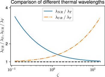
Figure 1. Comparison between λT and λNR, λUR.
By use of the relativistic thermal de Broglie wavelength λT , we can recast the expressions for $\bar{n}$ in the form
$\begin{eqnarray*}\bar{n}=\displaystyle \frac{1}{{({\lambda }_{T})}^{3}}{{\rm{e}}}^{-\alpha -\zeta }=\displaystyle \frac{1}{{({\lambda }_{T})}^{3}}{{\rm{e}}}^{(\bar{\mu }-{{mc}}^{2})/{k}_{{\rm{B}}}\bar{T}}.\end{eqnarray*}$
If the particle under consideration has some intrinsic quantum number, then the above expression needs to be multiplied by the corresponding intrinsic quantum degeneracy ${\mathfrak{g}}$, i.e.
$\begin{eqnarray}\bar{n}=\displaystyle \frac{{\mathfrak{g}}}{{({\lambda }_{T})}^{3}}{{\rm{e}}}^{-\alpha -\zeta }=\displaystyle \frac{{\mathfrak{g}}}{{({\lambda }_{T})}^{3}}{{\rm{e}}}^{(\bar{\mu }-{{mc}}^{2})/{k}_{{\rm{B}}}\bar{T}}.\end{eqnarray}$
This expression allows us to get a refined version of the famous Saha equation [23] which is related to the local ‘chemical equilibrium' for systems containing several different species of particles among which chemical reactions (or ionizations/recombinations) may take place. Let us assume that the system contains three different particle species A, B, C among which C = AB is the composite particle that may come as the result of the chemical reaction
$\begin{eqnarray*}A+B\rightleftharpoons C.\end{eqnarray*}$
Assume also that the interaction between different particles is negligible unless they collide and/or make the above chemical reaction. Under the above assumptions, the chemical potentials for different particle species satisfy the condition ${\bar{\mu }}_{A}+{\bar{\mu }}_{B}={\bar{\mu }}_{C}$ if the chemical reaction reaches a local equilibrium. Therefore, it follows from equation (42) that
$\begin{eqnarray}\displaystyle \frac{{\bar{n}}_{A}{\bar{n}}_{B}}{{\bar{n}}_{C}}=\displaystyle \frac{{{\mathfrak{g}}}_{A}{{\mathfrak{g}}}_{B}}{{{\mathfrak{g}}}_{C}}{\left(\displaystyle \frac{{\lambda }_{T}^{(C)}}{{\lambda }_{T}^{(A)}{\lambda }_{T}^{(B)}}\right)}^{3}{{\rm{e}}}^{-{\rm{\Delta }}E/{k}_{{\rm{B}}}\bar{T}},\end{eqnarray}$
where ΔE = (mA + mBmC)c2 is the binding energy of the composite particle C. If λT takes the form of equation (40), then equation (43) is precisely the famous Saha equation. However, as we have shown in section 3, λT actually takes the form (39), which is different from (40) unless ζ ≫ 1. Therefore, at smaller coldness (or higher temperature), equation (43) gives a relativistically refined version of the standard Saha equation. For gaseous systems with a single species of atoms which have several ionized states, equation (43) reduces to
$\begin{eqnarray*}\displaystyle \frac{{\bar{n}}_{i+1}{\bar{n}}_{e}}{{\bar{n}}_{i}}=2\displaystyle \frac{{{\mathfrak{g}}}_{i+1}}{{{\mathfrak{g}}}_{i}}\displaystyle \frac{1}{{\left({\lambda }_{T}^{(e)}\right)}^{3}}{{\rm{e}}}^{-{\rm{\Delta }}{E}_{i+1}/{k}_{{\rm{B}}}\bar{T}},\end{eqnarray*}$
where ${\bar{n}}_{i}$ is the number density of the atom in the ith ionized state, ΔEi+1 is the energy required to remove the (i + 1)th electron, and ${\lambda }_{T}^{(e)}$ is the relativistic thermal de Broglie wavelength for the electron.

6. Concluding remarks

Relativistic kinetic theory is a powerful tool for analyzing macroscopic behaviors for systems undergoing relativistic motion. In this work, using relativistic kinetic theory, we considered the longstanding problem of the relativistic transformation rules for some basic thermodynamic quantities, including the temperature T and the chemical potential μ. The major results are listed as follows:
$\begin{eqnarray*}\begin{array}{rcl}T & = & {\gamma }^{-1}\bar{T},\quad s=\gamma \bar{s},\quad \mu ={\gamma }^{-1}\bar{\mu },\\ n & = & \gamma \bar{n},\quad P=\bar{P},\quad w={\gamma }^{2}\bar{w},\end{array}\end{eqnarray*}$
wherein γ is the (local) Lorentz factor, and quantities with/without a bar are respectively measured by an instantaneous comoving observer $\bar{{ \mathcal O }}$ and an arbitrary instantaneous observer ${ \mathcal O }$, which are interrelated by a (local) Lorentz boost. These transformation rules, supplemented with the well-acknowledged contraction rule $\delta v={\gamma }^{-1}\delta \bar{v}$ for spatial volume element δv, constitute a complete set of transformation rules for all thermodynamic parameters which hold in both Minkowski and Rindler spacetimes, and we do not see any reason why they would not hold in other spacetimes. The transformation rule for T suggests that a moving body appears to be colder, supporting the first view by de Broglie, Einstein, and Planck et al. Moreover, our study adds some novel elements to the existing transformation rules; for instance, the rules for chemical potential and enthalpy density have not been reported elsewhere.
In the case of a perfect Rindler fluid, if we place the fluid in a box whose bottom is parallel to the Rindler horizon and let the bottom be located sufficiently close to the horizon, then our calculation shows that the total entropy and the total number of particles are proportional to the area of the bottom of the box, and both are independent of the height of the box. By extending to spacetimes with event horizons, a similar analysis might help to understand the area law of black hole entropy.
Finally, the exact results for the particle number density allow us to get a relativistically refined version of the famous Saha equation. At extremely high temperatures, or in the ultra-relativistic limits, the refinement could be significant, as in these cases the relativistic thermal de Broglie wavelength (39) could be significantly different from its non-relativistic counterpart (40).

Acknowledgments

This work is supported by the National Natural Science Foundation of China under grant No. 11575088, Hebei NSF under grant No. A2021205037 and the fund of Hebei Normal University under grant No. L2020B04. XH would like to thank Shao-Jiang Wang and Bin Wu for useful discussions.

Appendix

In the literature on relativistic kinetic theory, the expressions of local equilibrium quantities are mostly presented in a concrete spacetime dimension, mostly taken to be 4. In case one may be interested in the physical rules in generic spacetime dimensions, we now present the detailed calculations for all the macroscopic densities used in the main text in (d + 1)-dimensional Minkowski spacetime.
Let us start with the Cartesian coordinates and take the Killing vector field ${{ \mathcal B }}^{\mu }$ to be ${{ \mathcal B }}^{\mu }=\beta {({\partial }_{t})}^{\mu }=\beta {\bar{Z}}^{\mu }$. In these coordinates we can always parametrize pμ and Zμ as
$\begin{eqnarray*}\begin{array}{l}{p}^{\mu }={mc}(\cosh \theta ,\,\sinh \theta \cos {\theta }_{d-1},\\ \quad \sinh \theta \sin {\theta }_{d-1}\cos {\theta }_{d-2},\cdots ,\\ \quad \,\sinh \theta \sin {\theta }_{d-1}\cdots \sin {\theta }_{2}\cos {\theta }_{1},\\ \quad \sinh \theta \sin {\theta }_{d-1}\cdots \sin {\theta }_{2}\sin {\theta }_{1}),\\ {Z}^{\mu }=c(\cosh \eta ,\,\sinh \eta \cos {{\rm{\Theta }}}_{d-1},\\ \quad \sinh \eta \sin {{\rm{\Theta }}}_{d-1}\cos {{\rm{\Theta }}}_{d-2},\cdots \\ \quad \sinh \theta \sin {{\rm{\Theta }}}_{d-1}\cdots \sin {{\rm{\Theta }}}_{2}\cos {{\rm{\Theta }}}_{1},\\ \quad \sinh \theta \sin {{\rm{\Theta }}}_{d-1}\cdots \sin {{\rm{\Theta }}}_{2}\sin {{\rm{\Theta }}}_{1}),\end{array}\end{eqnarray*}$
where θ1, Θ1 ∈ [0, 2π), and θi, Θi ∈ [0, π) for i ≥ 2. To make the above parametrization also work for d = 1, we also introduce θ0 = Θ0 = 0.
It is straightforward to check that pμ and Zμ parametrized as above automatically satisfy the on-shell conditions p2 = − m2c2, Z2 = − c2, and
$\begin{eqnarray*}\begin{array}{l}\,| \vec{p}| \,=\,\sqrt{{\left({p}^{1}\right)}^{2}+{\left({p}^{2}\right)}^{2}+\cdots +{\left({p}^{d}\right)}^{2}}\\ \,=\,{mc}\sinh \theta ,\\ {\rm{d}}| \vec{p}| ={p}^{0}{\rm{d}}\theta =| {p}_{0}| {\rm{d}}\theta ,\end{array}\end{eqnarray*}$
so the momentum space volume element reads
$\begin{eqnarray*}\begin{array}{rcl}\varpi & = & \displaystyle \frac{{{\rm{d}}}^{d}{\rm{p}}}{| {p}_{0}| }=\displaystyle \frac{| \vec{p}{| }^{d-1}{\rm{d}}| \vec{p}| \,{\rm{d}}{{\rm{\Omega }}}_{d-1}}{| {p}_{0}| }\\ & = & {({mc}\sinh \theta )}^{d-1}{\rm{d}}\theta \,{\rm{d}}{{\rm{\Omega }}}_{d-1},\end{array}\end{eqnarray*}$
where for d = 1 dΩ0 = 1, and for d ≥ 2, ${\rm{d}}{{\rm{\Omega }}}_{d-1}={\sin }^{d-2}{\theta }_{d-1}{\rm{d}}{\theta }_{d-1}{\rm{d}}{{\rm{\Omega }}}_{d-2}$. The coordinate choice freedom allows us to set Θd−1 = 0, which greatly simplifies the forthcoming calculations. Moreover, comparing ${\bar{Z}}^{\mu }$ with Zμ and considering the relation (18), one recognizes that $\gamma =\cosh \eta $ is precisely the Lorentz factor related to the boost between the observers $\bar{{ \mathcal O }}$ and ${ \mathcal O }$.
Before delving into the analysis, we recall the following three integral representations for the modified Bessel function of the second kind, which are frequently used in our calculations,
$\begin{eqnarray}{K}_{\nu }(\zeta )={\int }_{0}^{\infty }{{\rm{e}}}^{-\zeta \cosh \theta }\cosh (\nu \theta ){\rm{d}}\theta ,\end{eqnarray}$
$\begin{eqnarray}\begin{array}{l}{K}_{\nu }(\zeta )={\left(\displaystyle \frac{\zeta }{2}\right)}^{\nu }\displaystyle \frac{\sqrt{\pi }}{{\rm{\Gamma }}\left(\nu +\tfrac{1}{2}\right)}\\ \quad {\,\times \int }_{0}^{\infty }{\sinh }^{2\nu }\theta \,{{\rm{e}}}^{-\zeta \cosh \theta }{\rm{d}}\theta ,\end{array}\end{eqnarray}$
$\begin{eqnarray}\begin{array}{l}{K}_{\nu }(\zeta )={\left(\displaystyle \frac{\zeta }{2}\right)}^{\nu }\displaystyle \frac{{\rm{\Gamma }}\left(\tfrac{1}{2}\right)}{{\rm{\Gamma }}\left(n+\tfrac{1}{2}\right)}\\ \quad \times {\int }_{1}^{\infty }{{\rm{e}}}^{-\zeta \theta }{\left({\theta }^{2}-1\right)}^{\nu -\tfrac{1}{2}}{\rm{d}}\theta .\end{array}\end{eqnarray}$
From the integral representation (A2), we can get
$\begin{eqnarray*}\begin{array}{l}{\left(\displaystyle \frac{{\rm{d}}}{{\rm{d}}\zeta }\right)}^{l}\left[\displaystyle \frac{{K}_{\nu }(\zeta )}{{\zeta }^{\nu }}\right]=\displaystyle \frac{{\left(-1\right)}^{l}\sqrt{\pi }}{{2}^{\nu }\,{\rm{\Gamma }}\left(\nu +\tfrac{1}{2}\right)}\\ \quad \times {\int }_{0}^{\infty }{\rm{d}}\theta {\sinh }^{2\nu }\theta {\cosh }^{l}\theta \,{{\rm{e}}}^{-\zeta \cosh \theta }.\end{array}\end{eqnarray*}$
On the other hand, from the representation (A3) we obtain the recurrence relations
$\begin{eqnarray*}{\left(\displaystyle \frac{{\rm{d}}}{\zeta {\rm{d}}\zeta }\right)}^{l}\left[\displaystyle \frac{{K}_{\nu }(\zeta )}{{\zeta }^{\nu }}\right]={\left(-1\right)}^{l}\displaystyle \frac{{K}_{\nu +l}(\zeta )}{{\zeta }^{\nu +l}}.\end{eqnarray*}$
It follows that
$\begin{eqnarray*}\begin{array}{l}{\int }_{0}^{\infty }{\rm{d}}\theta {\sinh }^{2\nu }\theta \,{{\rm{e}}}^{-\zeta \cosh \theta }\\ \quad =\displaystyle \frac{1}{\sqrt{\pi }}{\left(\displaystyle \frac{2}{\zeta }\right)}^{\nu }{\rm{\Gamma }}\left(\nu +\displaystyle \frac{1}{2}\right){K}_{\nu }(\zeta ),\\ {\int }_{0}^{\infty }{\rm{d}}\theta {\sinh }^{2\nu }\theta \cosh \theta \,{{\rm{e}}}^{-\zeta \cosh \theta }\\ \quad =\displaystyle \frac{1}{\sqrt{\pi }}{\left(\displaystyle \frac{2}{\zeta }\right)}^{\nu }{\rm{\Gamma }}\left(\nu +\displaystyle \frac{1}{2}\right){K}_{\nu +1}(\zeta ),\\ {\int }_{0}^{\infty }{\rm{d}}\theta {\sinh }^{2\nu }\theta {\cosh }^{2}\theta \,{{\rm{e}}}^{-\zeta \cosh \theta }\\ \quad =\displaystyle \frac{1}{\sqrt{\pi }}{\left(\displaystyle \frac{2}{\zeta }\right)}^{\nu }{\rm{\Gamma }}\left(\nu +\displaystyle \frac{1}{2}\right)\left[{K}_{\nu +2}(\zeta )-{\zeta }^{-1}{K}_{\nu +1}\right].\end{array}\end{eqnarray*}$
These integrations are sufficient for us to analyze the following observable quantities:
$\begin{eqnarray}n=-\displaystyle \frac{1}{{c}^{2}}{Z}_{\mu }{N}^{\mu }=-\displaystyle \frac{{{\rm{e}}}^{-\alpha }}{{{ch}}^{d}}\int \displaystyle \frac{{{\rm{d}}}^{d}\ {p}}{| {p}_{0}| }{Z}_{\mu }{p}^{\mu }{{\rm{e}}}^{{{ \mathcal B }}_{\mu }{p}^{\mu }},\end{eqnarray}$
$\begin{eqnarray}\epsilon =\displaystyle \frac{1}{{c}^{2}}{Z}_{\mu }{Z}_{\nu }{T}^{\mu \nu }=\displaystyle \frac{{{\rm{e}}}^{-\alpha }}{{{ch}}^{d}}\int \displaystyle \frac{{{\rm{d}}}^{d}\ {p}}{| {p}_{0}| }{\left({Z}_{\mu }{p}^{\mu }\right)}^{2}{{\rm{e}}}^{{{ \mathcal B }}_{\mu }{p}^{\mu }},\end{eqnarray}$
$\begin{eqnarray}\begin{array}{rcl}{ \mathcal T } & = & \displaystyle \frac{c\,{{\rm{e}}}^{-\alpha }}{{h}^{d}}\int \displaystyle \frac{\sqrt{g}\,{{\rm{d}}}^{d}p}{| {p}_{0}| }{p}^{2}{{\rm{e}}}^{{{ \mathcal B }}_{\rho }{p}^{\rho }}\\ & = & -\displaystyle \frac{{m}^{2}{c}^{3}{{\rm{e}}}^{-\alpha }}{{h}^{d}}\int \displaystyle \frac{{{\rm{d}}}^{d}{p}}{| {p}_{0}| }{{\rm{e}}}^{{{ \mathcal B }}_{\mu }{p}^{\mu }},\end{array}\end{eqnarray}$
where ${{ \mathcal B }}_{\mu }{p}^{\mu }=\zeta \cosh \theta $ where ζ is the relativistic coldness, and the contraction Zμpμ is simplified after taking Θd−1 = 0:
$\begin{eqnarray*}\begin{array}{l}{Z}_{\mu }{p}^{\mu }={{mc}}^{2}\left(\sinh \eta \sinh \theta \cos {\theta }_{d-1}\right.\\ \quad \left.-\cosh \eta \cosh \theta \right)={{mc}}^{2}{ \mathcal C }(\eta ,\theta ,{\theta }_{d-1}).\end{array}\end{eqnarray*}$
When d = 1 there is only one spatial direction and the above integrations can be carried out with ease. First, the trace of the energy-momentum tensor reads
$\begin{eqnarray}\begin{array}{rcl}{ \mathcal T } & = & -\displaystyle \frac{{{\rm{e}}}^{-\alpha }}{{\lambda }_{C}}{{mc}}^{2}{\int }_{-\infty }^{+\infty }{\rm{d}}\theta {{\rm{e}}}^{-\zeta \cosh \theta }\\ & = & -\displaystyle \frac{2{{\rm{e}}}^{-\alpha }}{{\lambda }_{C}}{{mc}}^{2}{K}_{0}(\zeta ).\end{array}\end{eqnarray}$
For the particle number density and energy density, after a few lines of simple calculations we obtain
$\begin{eqnarray}\begin{array}{rcl}n & = & -\displaystyle \frac{{{\rm{e}}}^{-\alpha }}{{\lambda }_{C}}{\int }_{-\infty }^{\infty }{\rm{d}}\theta \left(\sinh \eta \sinh \theta \right.\\ & & \left.-\cosh \eta \cosh \theta \right){{\rm{e}}}^{-\zeta \cosh \theta }\\ & = & \displaystyle \frac{2{{\rm{e}}}^{-\alpha }}{{\lambda }_{C}}\cosh \eta {\int }_{0}^{\infty }{\rm{d}}\theta \cosh \theta {{\rm{e}}}^{-\zeta \cosh \theta }\\ & = & \gamma \displaystyle \frac{2{{\rm{e}}}^{-\alpha }}{{\lambda }_{C}}{K}_{1}(\zeta ),\end{array}\end{eqnarray}$
and
$\begin{eqnarray}\begin{array}{rcl}\epsilon & = & \displaystyle \frac{{{\rm{e}}}^{-\alpha }}{{\lambda }_{C}}{{mc}}^{2}{\int }_{-\infty }^{\infty }{\rm{d}}\theta \left(\sinh \eta \sinh \theta \right.\\ & & {\left.-\cosh \eta \cosh \theta \right)}^{2}{{\rm{e}}}^{-\zeta \cosh \theta }\\ & = & \displaystyle \frac{2{{\rm{e}}}^{-\alpha }}{{\lambda }_{C}}{{mc}}^{2}{\int }_{0}^{\infty }{\rm{d}}\theta \left[{\gamma }^{2}\cosh 2\theta \right.\\ & & \left.-{\sinh }^{2}\theta \right]{{\rm{e}}}^{-\zeta \cosh \theta }\\ & = & \displaystyle \frac{2{{\rm{e}}}^{-\alpha }}{{\lambda }_{C}}{{mc}}^{2}\left[{\gamma }^{2}{K}_{2}(\zeta )-\displaystyle \frac{{K}_{1}(\zeta )}{\zeta }\right].\end{array}\end{eqnarray}$
When d ≥ 2, the integrations (A4)-(A6) can be evaluated in a unified way:
$\begin{eqnarray}\begin{array}{l}n=-\displaystyle \frac{{{\rm{e}}}^{-\alpha }}{{\lambda }_{C}^{d}}\int {\rm{d}}{{\rm{\Omega }}}_{d-1}{\int }_{0}^{\infty }{\rm{d}}\theta \\ \quad \times {\sinh }^{d-1}\theta \,{ \mathcal C }(\eta ,\theta ,{\theta }_{d-1}){{\rm{e}}}^{-\zeta \cosh \theta }\\ \quad =\displaystyle \frac{{{\rm{e}}}^{-\alpha }}{{\lambda }_{C}^{d}}\cosh \eta \int {\rm{d}}{{\rm{\Omega }}}_{d-1}{\int }_{0}^{\infty }{\rm{d}}\theta \\ \quad \times {\sinh }^{d-1}\theta \cosh \theta \,{{\rm{e}}}^{-\zeta \cosh \theta }\\ \quad =\displaystyle \frac{{{ \mathcal A }}_{d-1}{{\rm{e}}}^{-\alpha }}{{\lambda }_{C}^{d}}\gamma {\int }_{0}^{\infty }{\rm{d}}\theta {\sinh }^{d-1}\theta \\ \quad \times \cosh \theta \,{{\rm{e}}}^{-\zeta \cosh \theta }\\ \quad =\gamma \displaystyle \frac{2\,{{\rm{e}}}^{-\alpha }}{{\lambda }_{C}^{d}}{\left(\displaystyle \frac{2\pi }{\zeta }\right)}^{\tfrac{d-1}{2}}{K}_{\tfrac{d+1}{2}}(\zeta ),\end{array}\end{eqnarray}$
where ${{ \mathcal A }}_{d-1}=\int {\rm{d}}{{\rm{\Omega }}}_{d-1}=\tfrac{2{\pi }^{d/2}}{{\rm{\Gamma }}\left(\tfrac{d}{2}\right)}$ is the area of a (d − 1)-dimensional unit sphere,
$\begin{eqnarray}\begin{array}{rcl}\epsilon & = & \displaystyle \frac{{{\rm{e}}}^{-\alpha }}{{\lambda }_{C}^{d}}{{mc}}^{2}\int {\rm{d}}{{\rm{\Omega }}}_{d-1}{\int }_{0}^{\infty }{\rm{d}}\theta \\ & & {\times \sinh }^{d-1}\theta \,{{ \mathcal C }}^{2}(\eta ,\theta ,{\theta }_{d-1})\,{{\rm{e}}}^{-\zeta \cosh \theta }\\ & = & \displaystyle \frac{{{\rm{e}}}^{-\alpha }}{{\lambda }_{C}^{d}}{{mc}}^{2}\left[{\gamma }^{2}{{ \mathcal A }}_{d-1}{\int }_{0}^{\infty }{\rm{d}}\theta \right.\\ & & {\times \sinh }^{d-1}\theta {\cosh }^{2}\theta \,{{\rm{e}}}^{-\zeta \cosh \theta }\\ & & +({\gamma }^{2}-1){{ \mathcal A }}_{d-2}\displaystyle \frac{\sqrt{\pi }}{2}\displaystyle \frac{{\rm{\Gamma }}\left(\tfrac{d-1}{2}\right)}{{\rm{\Gamma }}\left(\tfrac{d}{2}+1\right)}\\ & & \left.\times {\int }_{0}^{\infty }{\rm{d}}\theta {\sinh }^{d+1}\theta \,{{\rm{e}}}^{-\zeta \cosh \theta }\right]\\ & = & \displaystyle \frac{{{\rm{e}}}^{-\alpha }}{{\lambda }_{C}^{d}}{{mc}}^{2}{{ \mathcal A }}_{d-1}{\int }_{0}^{\infty }{\rm{d}}\theta \left[{\gamma }^{2}{\sinh }^{d-1}\theta {\cosh }^{2}\theta \right.\\ & & \left.+\displaystyle \frac{{\gamma }^{2}-1}{d}{\sinh }^{d+1}\theta \right]{{\rm{e}}}^{-\zeta \cosh \theta }\\ & = & \displaystyle \frac{{{\rm{e}}}^{-\alpha }}{{\lambda }_{C}^{d}}\displaystyle \frac{{{ \mathcal A }}_{d-1}}{\sqrt{\pi }}{\left(\displaystyle \frac{2}{\zeta }\right)}^{\tfrac{d-1}{2}}{\rm{\Gamma }}\left(\displaystyle \frac{d}{2}\right){{mc}}^{2}\\ & & \times \left[{\gamma }^{2}\left({K}_{\tfrac{d+3}{2}}-{\zeta }^{-1}{K}_{\tfrac{d+1}{2}}\right)\right.\\ & & \left.+\displaystyle \frac{{\gamma }^{2}-1}{d}\displaystyle \frac{2}{\zeta }\displaystyle \frac{d}{2}{K}_{\tfrac{d+1}{2}}\right]\\ & = & \displaystyle \frac{2\,{{\rm{e}}}^{-\alpha }}{{\lambda }_{C}^{d}}{\left(\displaystyle \frac{2\pi }{\zeta }\right)}^{\tfrac{d-1}{2}}{{mc}}^{2}\\ & & \times \left[{\gamma }^{2}{K}_{\tfrac{d+3}{2}}(\zeta )-{\zeta }^{-1}{K}_{\tfrac{d+1}{2}}(\zeta )\right],\end{array}\end{eqnarray}$
and
$\begin{eqnarray}\begin{array}{rcl}{ \mathcal T } & = & -\displaystyle \frac{{{\rm{e}}}^{-\alpha }}{{\lambda }_{C}^{d}}{{ \mathcal A }}_{d-1}{{mc}}^{2}{\int }_{0}^{\infty }{\rm{d}}\theta {\sinh }^{d-1}\theta \,{{\rm{e}}}^{-\zeta \cosh \theta }\\ & = & -\displaystyle \frac{{{\rm{e}}}^{-\alpha }}{{\lambda }_{C}^{d}}\displaystyle \frac{{{ \mathcal A }}_{d-1}}{\sqrt{\pi }}{\left(\displaystyle \frac{2}{\zeta }\right)}^{\tfrac{d-1}{2}}{\rm{\Gamma }}\left(\displaystyle \frac{d}{2}\right){{mc}}^{2}{K}_{\tfrac{d-1}{2}}(\zeta )\\ & = & -\displaystyle \frac{2\,{{\rm{e}}}^{-\alpha }}{{\lambda }_{C}^{d}}{\left(\displaystyle \frac{2\pi }{\zeta }\right)}^{\tfrac{d-1}{2}}{{mc}}^{2}{K}_{\tfrac{d-1}{2}}(\zeta ).\end{array}\end{eqnarray}$
Interestingly, the results (A10)-(A12) calculated for d ≥ 2 are also valid for d = 1, as we have shown in equations (A7)-(A9).
For the thermodynamic pressure, we refer to (24), with the replacement $\tfrac{1}{3}\to \tfrac{1}{d}$. By evaluating the isotropic pressure in the rest frame where γ = 1, we get
$\begin{eqnarray}\begin{array}{rcl}P & = & \bar{P}=\displaystyle \frac{{ \mathcal T }+\bar{\epsilon }}{d}=\displaystyle \frac{2\,{{\rm{e}}}^{-\alpha }}{{\lambda }_{C}^{d}}\\ & & \times {\left(\displaystyle \frac{2\pi }{\zeta }\right)}^{\tfrac{d-1}{2}}{\zeta }^{-1}{{mc}}^{2}{K}_{\tfrac{d+1}{2}}(\zeta ),\end{array}\end{eqnarray}$
and finally the enthalpy density is obtained to be
$\begin{eqnarray}\begin{array}{l}w=\epsilon +P={\gamma }^{2}\\ \quad \times \left[\displaystyle \frac{2\,{{\rm{e}}}^{-\alpha }}{{\lambda }_{C}^{d}}{\left(\displaystyle \frac{2\pi }{\zeta }\right)}^{\tfrac{d-1}{2}}\right]{{mc}}^{2}{K}_{\tfrac{d+3}{2}}(\zeta ).\end{array}\end{eqnarray}$
This finishes our calculations for the relevant quantities in arbitrary dimensions.
1
de Broglie L 1907 Diverses Questions de Mécanique et de Thermodynamique Classiques et Relativistes Berlin, Heidelberg Springer p 146

2
Einstien A 1907 Über das Relativitätsprinzip und die aus demselben gezogenen Folgerungenn Jahrb. Radioakt. Elektron. 4 411 462

3
Planck M 1908 Zur dynamik bewegter systeme Ann. Phys. 331 1 34

DOI

4
Eddington A S 1923 The Mathematical Theory of Relativity Cambridge University Press p 34

5
Ott H 1963 Lorentz-transformation der Wärme und der temperatur Zeitschrift für Physik 175 70 104

DOI

6
Arzelies H 1965 Transformation relativiste de la température et de quelques autres grandeurs thermodynamiques Il Nuovo Cimento 35 792 804

DOI

7
Landsberg P T 1966 Does a moving body appear cool? Nature 212 571 572

DOI

8
Landsberg P T 1967 Does a moving body appear cool? Nature 214 903 904

DOI

9
Cavalleri G Salgarelli G 1969 Revision of the relativistic dynamics with variable rest mass and application to relativistic thermodynamics Il Nuovo Cimento A 62 722 754

DOI

10
Newburgh R G 1979 Relativistic thermodynamics: temperature transformations, invariance and measurement Il Nuovo Cimento B 52 219 228

DOI

11
Liu C 1979 Einstein and relativistic thermodynamics in 1952: a historical and critical study of a strange episode in the history of modern physics Br. J. Hist. Sci. 25 185 206

DOI

12
Landsberg P T Matsas G E A 2004 The impossibility of a universal relativistic temperature transformation Physica A 340 92 94

DOI

13
Landsberg P T Matsas G E A 1996 Laying the ghost of the relativistic temperature transformation Phys. Lett. A 223 401 403

DOI

14
Farías C Pinto V A Moya P S 2017 What is the temperature of a moving body? Sci. Rep. 7 17657

DOI

15
Kolekar S Padmanabhan T 2011 Ideal gas in a strong gravitational field: area dependence of entropy Phys. Rev. D 83 064034

DOI

16
Bhattacharya S Chakraborty S Padmanabhan T 2017 Entropy of a box of gas in an external gravitational field revisited Phys. Rev. D 96 084030

DOI

17
Kim H-C Ji C-R 2017 Matter equation of state in general relativity Phys. Rev. D 95 084045

DOI

18
Li D Wu B Xu Z M Yang W L 2021 A shell of bosons in spherically symmetric spacetimes Phys. Lett. B 820 136588

DOI

19
Cubero D Casado-Pascual J Dunkel J Talkner P Hänggi P 2007 Thermal equilibrium and statistical thermometers in special relativity Phys. Rev. Lett. 99 170601

DOI

20
Montakhab A Ghodrat M Barati M 2009 Statistical thermodynamics of a two-dimensional relativistic gas Phys. Rev. E 79 031124

DOI

21
Kaniadakis G 2002 Statistical mechanics in the context of special relativity Phys. Rev. E 65 056125

DOI

22
Jüttner F 1911 Das maxwellsche gesetz der geschwindigkeitsverteilung in der relativtheorie Ann. Phys. 339 856 882

DOI

23
Saha M N 1920 Ionization in the solar chromosphere London, Edinburgh Dublin Philos. Mag. J. Sci. 40 472 488

DOI

24
Sarbach O Zannias T 2013 Relativistic kinetic theory: an introduction AIP Conf. Proc. 1548 134 155

25
Sarbach O Zannias T 2014 The geometry of the tangent bundle and the relativistic kinetic theory of gases Class. Quant. Grav. 31 085013

DOI

26
De Groot S R Van Leeuwen W A Van Weert C G 1980 Relativistic Kinetic Theory. Principles and Applications North-Holland

27
Cercignani C Kremer G M 2002 The Relativistic Boltzmann Equation: Theory and Applications Basel Birkhäuser

28
Hakim R 2011 Introduction to Relativistic Statistical Mechanics: Classical and Quantum World Scientific

29
Israel W Stewart J M 1979 Transient relativistic thermodynamics and kinetic theory Ann. Phys. 118 341 372

DOI

30
Tolman R C Ehrenfest P 1930 Temperature equilibrium in a static gravitational field Phys. Rev. 36 1791 1798

DOI

Outlines

/