Welcome to visit Communications in Theoretical Physics,
Quantum Physics and Quantum Information

Optimality of T-gate for generating magic resource

  • Xiaohui Li 1, 2 ,
  • Shunlong Luo , 1, 2
Expand
  • 1Academy of Mathematics and Systems Science, Chinese Academy of Sciences, Beijing 100190, China
  • 2School of Mathematical Sciences, University of Chinese Academy of Sciences, Beijing 100049, China

Received date: 2022-10-09

  Revised date: 2022-12-29

  Accepted date: 2022-12-30

  Online published: 2023-04-24

Copyright

© 2023 Institute of Theoretical Physics CAS, Chinese Physical Society and IOP Publishing

Abstract

In the stabilizer formalism of fault-tolerant quantum computation, stabilizer states serve as classical objects, while magic states (non-stabilizer states) are a kind of quantum resource (called magic resource) for promoting stabilizer circuits to universal quantum computation. In this framework, the T-gate is widely used as a non-Clifford gate which generates magic resource from stabilizer states. A natural question arises as whether the T-gate is in some sense optimal for generating magic resource. We address this issue by employing an intuitive and computable quantifier of magic based on characteristic functions (Weyl transforms) of quantum states. We demonstrate that the qubit T-gate, as well as its qutrit extension, the qutrit T-gate, are indeed optimal for generating magic resource among the class of diagonal unitary operators. Moreover, up to Clifford equivalence, the T-gate is essentially the only gate having such an optimal property. This reveals some intrinsic optimal features of the T-gate. We further compare the T-gate with general unitary gates for generating magic resource.

Cite this article

Xiaohui Li , Shunlong Luo . Optimality of T-gate for generating magic resource[J]. Communications in Theoretical Physics, 2023 , 75(4) : 045101 . DOI: 10.1088/1572-9494/acaf28

1. Introduction

A convenient and popular framework for fault-tolerant quantum computation is the stabilizer formalism with magic state injection [122]. The celebrated Gottesman–Knill theorem shows that stabilizer circuits (composed of Clifford unitaries, Pauli measurements, conditioning on measurement outcomes, and classical randomness) can be efficiently simulated by classical computers [1, 8], while universal fault-tolerant quantum computation can be achieved via injection of magic states (non-stabilizer states) or magic-resource-generating gates (e.g. the T-gate) into stabilizer circuits [16].
Various protocols for magic state distillation, which generate more refined magic states from coarse ones have been extensively studied [6, 911, 1416, 21]. This is helpful in paving the way for generating magic resource in order to implement quantum computation via the stabilizer formalism and magic resource.
For controlling and manipulating magic resource, it is desirable to quantify the amount of magic (non-stabilizerness) from different perspectives. Many quantifiers of magic have been introduced in various contexts. For example, the sum negativity (with the associated mana and thauma) uses the negative part of the discrete Wigner functions as an indicator of magic [11, 20, 21]. The stabilizer rank, defined as the minimal number of components in the expansion of a state in terms of stabilizer states, was introduced in [13, 18]. The relative entropy of magic (with the associated max-relative entropy and min-relative entropy of magic), and the robustness of magic, were studied in [11, 15, 17]. Apart from the sum negativity, these quantifiers of magic are in general quite difficult to calculate. The sum negativity is computable, however, it relies heavily on the discrete Wigner functions in odd dimensions, which excludes its direct usage in other dimensions. In particular, the ubiquitous qubit case is excluded. It is desirable to seek easily computable quantifiers of magic applicable to all dimensions and not depending on the discrete Wigner functions [22].
The T-gate plays a crucial role in the Clifford +T gate set, which is approximately universal for fault-tolerant quantum computation [2335]. The qutrit version of the qubit T-gate is introduced in [10, 23, 27], and shares a variety of similar properties with the qubit T-gate. The T-count (the number of T-gate used in a circuit) is widely used as a benchmark for the complexity of a circuit [24, 25]. A basic feature of the T-gate lies in that it is a powerful and convenient gate for generating magic states from stabilizer states, and can be fault-tolerantly implemented.
In this context, a natural question arises as how powerful or optimal the T-gate is for generating magic resource. The present work is devoted to addressing this issue. For this purpose, we will employ a quantifier of magic based on characteristic functions (Weyl transforms) of quantum states to assess the power (capability) of quantum gates for generating magic resource. We will demonstrate that both the qubit T-gate and qutrit T-gate are optimal for generating magic resource in the class of diagonal unitary operators, and up to Clifford equivalence, they are essentially the only ones having this optimality.
The remainder of the work is structured as follows. In section 2, as preliminaries, we review some basic aspects of the stabilizer formalism, in which states are classified into stabilizer states and magic states, with the latter regarded as a magic resource serving as quantumness for promoting stabilizer circuits to universal quantum computation. In section 3, we study magic-resource-generating power of quantum gates (i.e. unitary operators) and reveal some optimal features of the T-gate for both qubit and qutrit systems. We employ characteristic functions (which are well-defined on all dimensions) rather than the discrete Wigner functions (which are only well-defined on odd dimensions) to construct a computable quantifier of magic. We consider both the maximal and average scenarios for quantifying magic-resource generating power. Finally, we present a summary and discussion in section 4. The detailed proof of the main result, proposition 2, is presented in the appendix.

2. Preliminaries: stabilizer states and magic states

In this section, we review the basic features of the stabilizer formalism, which plays an important role in quantum error correction and fault-tolerant quantum computation [19, 1122]. The Pauli group (discrete Heisenberg-Weyl group) and the Clifford group are basic ingredients for constructing stabilizer circuits, which can be efficiently simulated by classical means, while non-Clifford gates such as the T-gate are necessary for universal quantum computation.
We first recall the Pauli group, which will play a crucial role in this work. For a d-dimensional quantum system ${{\mathbb{C}}}^{d}$ with computational basis $\{| j\rangle :j\in {{\mathbb{Z}}}_{d}\}$, we may regard ${{\mathbb{Z}}}_{d}=\{0,1,\cdots ,d-1\}$ (the ring of integers modulo d) as a discrete configuration space of this system, and identify ${L}^{2}({{\mathbb{Z}}}_{d})$ (the set of complex functions on ${{\mathbb{Z}}}_{d}$) with ${{\mathbb{C}}}^{d},$ regarded naturally as a finite-dimensional Hilbert space. In this space, two fundamental unitary operators [36]
$\begin{eqnarray*}X=\displaystyle \sum _{k=0}^{d-1}| k+1\rangle \langle k| ,\quad Z=\displaystyle \sum _{k=0}^{d-1}{\omega }^{k}| k\rangle \langle k| ,\qquad \omega ={{\rm{e}}}^{2\pi {\rm{i}}/d},\end{eqnarray*}$
emerge naturally and serve as building blocks for finite-dimensional quantum mechanics. Clearly,
$\begin{eqnarray*}X| k\rangle =| k+1\rangle ,\quad Z| k\rangle ={\omega }^{k}| k\rangle ,\quad k\in {{\mathbb{Z}}}_{d}.\end{eqnarray*}$
The arithmetic is modular d, and thus ∣d⟩ = ∣0⟩. Associated with these two basic operators, the discrete Heisenberg-Weyl operators are defined as
$\begin{eqnarray*}{D}_{k,l}={\tau }^{{kl}}{X}^{k}{Z}^{l},\quad k,l\in {\mathbb{Z}},\end{eqnarray*}$
where $\tau =-{{\rm{e}}}^{\pi {\rm{i}}/d}=-\sqrt{\omega }.$ Here we emphasize that Dk,l are well defined for all $k,l\in {\mathbb{Z}},$ though we will mainly consider $k,l\in {{\mathbb{Z}}}_{d}.$ We call $(k,l)\in {{\mathbb{Z}}}_{d}\times {{\mathbb{Z}}}_{d}$ (discrete phase-space) a phase-space point. The discrete Heisenberg-Weyl operators constitute a projective representation of the translation groups ${{\mathbb{Z}}}_{d}\times {{\mathbb{Z}}}_{d}$ and ${\mathbb{Z}}\times {\mathbb{Z}},$ and satisfy
$\begin{eqnarray}{D}_{k,l}{D}_{s,t}={\tau }^{{ls}-{kt}}{D}_{k+s,l+t},\qquad k,l,s,t\in {\mathbb{Z}}.\end{eqnarray}$
Moreover,
$\begin{eqnarray*}\mathrm{tr}({D}_{k,l}{D}_{s,t}^{\dagger })=d{\delta }_{k,s}{\delta }_{l,t},\qquad k,l,s,t\in {{\mathbb{Z}}}_{d},\end{eqnarray*}$
and $\{\tfrac{1}{\sqrt{d}}{D}_{k,l}:k,l\in {{\mathbb{Z}}}_{d}\}$ constitutes an orthonormal basis for the d2-dimensional operator space $L({{\mathbb{C}}}^{d}),$ the set of all operators on ${{\mathbb{C}}}^{d}$ equipped with the Hilbert-Schmidt inner product $\langle A| B\rangle =\mathrm{tr}({A}^{\dagger }B).$
For the convenience of our approach, we take the Pauli group (discrete Heisenberg-Weyl group) as
$\begin{eqnarray*}{{ \mathcal P }}_{d}=\{{\tau }^{j}{D}_{k,l}:j\in {{\mathbb{Z}}}_{2d},k,l\in {{\mathbb{Z}}}_{d}\}.\end{eqnarray*}$
In particular, ${{ \mathcal P }}_{2}=\{c1,c{\sigma }_{x},c{\sigma }_{y},c{\sigma }_{z}:c=\pm 1,\pm {\rm{i}}\},$ with σx, σy, σz being the standard Pauli operators. The Clifford group
$\begin{eqnarray*}{{ \mathcal C }}_{d}=\{V\in {{ \mathcal U }}_{d}:V{{ \mathcal P }}_{d}{V}^{\dagger }={{ \mathcal P }}_{d}\}\end{eqnarray*}$
is the normalizer (natural symmetry group) of ${{ \mathcal P }}_{d}$ in the full unitary group ${{ \mathcal U }}_{d}$ on ${{\mathbb{C}}}^{d}.$ This group plays an instrumental role in the stabilizer quantum computation.
A stabilizer state is defined as a common eigenstate (with common eigenvalue 1) of a maximal Abelian subgroup of the Clifford group ${{ \mathcal C }}_{d}.$ In this context, the subgroup is called the stabilizer group of the stabilizer state. The set of (pure) stabilizer states in ${{\mathbb{C}}}^{d}$ is denoted by ${{ \mathcal S }}_{d},$ which consists exactly of $| {{ \mathcal S }}_{d}| =d(d+1)$ elements [7]. In prime power dimensions, any state of the form Vj⟩ is a stabilizer state. Here $| j\rangle \in {{\mathbb{C}}}^{d}$ is any computational basis state and $V\in {{ \mathcal C }}_{d}$ is any Clifford operator [7, 11]. Convex mixtures (i.e. probabilistic mixtures) of pure stabilizer states are called mixed stabilizer states. Any state (pure or mixed) that cannot be expressed as a convex mixture of pure stabilize states is called a magic state (non-stabilizer state). Any magic state is regarded as magic resource.
The sets of pure stabilizer states in ${{\mathbb{C}}}^{d}$ for d = 2 and 3 are listed in tables 1 and 2, respectively, which will be needed in the sequel.
Table 1. Qubit stabilizer states and the corresponding stabilizer generators, which stabilize the corresponding states and generate the corresponding maximal Abelian subgroups of ${{ \mathcal P }}_{2}$ stabilizing the corresponding states. For example, σx∣ + ⟩ = ∣ + ⟩, and σx generates the maximal Abelian subgroup {1, σx} stabilizing the state ∣ + ⟩. The three operators σx, σy and σz are the Pauli spin operators (matrices).
Stabilizer state ∣ + ⟩ ∣ − ⟩ ∣ + i⟩ ∣ − i⟩ ∣0⟩ ∣1⟩
Stabilizer generator σx σx σy σy σz σz
For the purpose of studying the power of quantum gates for generating magic resource, we need to quantify magic resource [11, 1422]. For any quantum state (pure or mixed) ρ on ${{\mathbb{C}}}^{d}$, we employ the following quantifier
$\begin{eqnarray}M(\rho )=\displaystyle \sum _{k,l\in {{\mathbb{Z}}}_{d}}| \mathrm{tr}(\rho {D}_{k,l})| \end{eqnarray}$
introduced in [22], which is easy to compute and has a variety of useful properties:
a

(a) $1\leqslant M(\rho )\leqslant 1+(d-1)\sqrt{d\,+\,1}.$

b

(b) M(ρ) is invariant under the Clifford operations in the sense that $M(V\rho {V}^{\dagger })=M(\rho ),\forall \ V\in {{ \mathcal C }}_{d}.$

c

(c) M(ρ) is convex in ρ.

d

(d) Among all states (pure or mixed), M(ρ) achieves the minimal value 1 if and only if ρ = 1/d is the maximally mixed state. In view of this property, one may prefer to employ M0(ρ) = M(ρ) − 1 as a more appropriate quantifier of magic. However, we will not make this convention.

e

(e) Among pure states, M(∣ψ⟩⟨ψ∣) achieves the minimal value d if and only if ∣ψ⟩ is a stabilizer state. Consequently, all pure stabilizer states have the same value of magic (i.e. d). In particular, by the above properties, we have the following simple criterion for non-stabilizerness (magic states): if M(ρ) > d, then the state ρ is magic. It should be noticed that this is only a sufficient, but not necessary, condition for a state on ${{\mathbb{C}}}^{d}$ to be magic.

A remarkable feature of M(ρ) is that it achieves the maximal value $1+(d-1)\sqrt{d\,+\,1}$ by any SIC-POVM fiducial state (assuming its existence, which has been proved in many dimensions) [22]. In particular, it is known that such fiducial states exist in many dimensions, including the cases d = 2, 3 [37, 38]. Recall that a SIC-POVM (symmetric informationally complete positive operator valued measure) in ${{\mathbb{C}}}^{d}$ is a POVM {Eα: α = 1, 2, ⋯ ,d2} (i.e. ${E}_{\alpha }\,\geqslant 0,{\sum }_{\alpha =1}^{{d}^{2}}{E}_{\alpha }={\bf{1}}$) consisting of d2 rank-one operators with equal trace and equal overlap and spanning the whole state space [37, 38]. It has been shown that SIC-POVMs exist in many dimensions, although the general existence remains an outstanding open problem (Zauner's conjecture) [3753]. A SIC-POVM fiducial state is a pure state $| f\rangle \in {{\mathbb{C}}}^{d}$ such that its orbit $\{{E}_{k,l}=\tfrac{1}{d}{D}_{k,l}| f\rangle \langle f| {D}_{k,l}^{\dagger }:k,l\in {{\mathbb{Z}}}_{d}\}$ under the Pauli group constitutes a SIC-POVM. Fiducial states have been explicitly constructed in many dimensions, and most SIC-POVMs are constructed from fiducial states [37, 38].
For any quantum gate described by a unitary operator U on ${{\mathbb{C}}}^{d},$ by employing M( · ) defined by equation (2) as a quantifier of magic, we introduce the following quantities
$\begin{eqnarray*}{M}_{\max }(U)=\mathop{\max }\limits_{| \psi \rangle \in {{ \mathcal S }}_{d}}M(U| \psi \rangle ),\end{eqnarray*}$
$\begin{eqnarray*}{M}_{\mathrm{ave}}(U)=\displaystyle \frac{1}{| {{ \mathcal S }}_{d}| }\displaystyle \sum _{| \psi \rangle \in {{ \mathcal S }}_{d}}M(U| \psi \rangle ),\end{eqnarray*}$
which characterize the maximal and average magic-resource-generating powers of U, respectively. Here $| {{ \mathcal S }}_{d}| =d(d+1)$ is the number of pure stabilizer states in ${{\mathbb{C}}}^{d}$ [7]. We will use these quantities to characterize the T-gate from an optimal perspective.

3. Optimality of T-gate for generating magic-resource

In this section, we evaluate explicitly the magic-resource-generating power of some unitary gates in the qubit (d = 2) and qutrit (d = 3) cases. In particular, we illuminate some optimal features of the T-gate: In these low dimensions, the T-gate is optimal for generating magic resource among the class of diagonal unitary gates.

3.1. Qubit T-gate

For a qubit system (d = 2) with computational basis {∣0⟩, ∣1⟩}, there are six pure stabilizer states [7, 16]
$\begin{eqnarray*}| \pm \rangle =\displaystyle \frac{1}{\sqrt{2}}(| 0\rangle \pm | 1\rangle ),\,| \pm {\rm{i}}\rangle =\displaystyle \frac{1}{\sqrt{2}}(| 0\rangle \pm {\rm{i}}| 1\rangle ),\,| 0\rangle ,| 1\rangle ,\end{eqnarray*}$
which correspond to the three pairs of antipodal points in the intersection of the three principal axes and the Bloch sphere, and may be partitioned into three mutually unbiased bases {∣ ± ⟩}, {∣ ± i⟩}, and {∣0⟩, ∣1⟩} for ${{\mathbb{C}}}^{2}.$ Geometrically, they constitute the vertex of the stabilizer octahedron inscribed in the qubit Bloch sphere. These states are listed in table 1 together with the corresponding stabilizer generators.
In magic state distillation and gate synthesis, the non-Clifford qubit T-gate [6]
$\begin{eqnarray}\begin{array}{rcl}{T}_{2} & = & | 0\rangle \langle 0| +{{\rm{e}}}^{{\rm{i}}\pi /4}| 1\rangle \langle 1| \\ & = & {{\rm{e}}}^{{\rm{i}}\pi /8}\left({{\rm{e}}}^{-{\rm{i}}\pi /8}| 0\rangle \langle 0| +{{\rm{e}}}^{{\rm{i}}\pi /8}| 1\rangle \langle 1| \right)\\ & = & \left(\begin{array}{cc}1 & 0\\ 0 & {{\rm{e}}}^{{\rm{i}}\pi /4}\end{array}\right),\end{array}\end{eqnarray}$
plays a prominent role and has been widely used as a benchmark for non-stabilizerness of qubit gates. Due to the presence of ±π/8 (corresponding to rotation with angle π/8), this T-gate is also called π/8-gate, and if one ignores the overall phase eiπ/8, one also regards e−iπ/8∣0⟩⟨0∣ + eiπ/8∣1⟩⟨1∣ as the π/8-gate.
To address the optimality of the qubit gate T2 defined by equation (3), consider the family of qubit diagonal unitary gates
$\begin{eqnarray}{U}_{\theta }=| 0\rangle \langle 0| +{{\rm{e}}}^{{\rm{i}}\theta }| 1\rangle \langle 1| =\left(\begin{array}{cc}1 & 0\\ 0 & {{\rm{e}}}^{{\rm{i}}\theta }\end{array}\right),\quad \theta \in [0,2\pi ),\end{eqnarray}$
which includes the T-gate T2 = Uπ/4 as a special instance. By simple and direct calculations, we have
$\begin{eqnarray*}M({U}_{\theta }| \pm \rangle )=M({U}_{\theta }| \pm {\rm{i}}\rangle )=1+| \cos \theta | +| \sin \theta | ,\end{eqnarray*}$
$\begin{eqnarray*}M({U}_{\theta }| 0\rangle )=M({U}_{\theta }| 1\rangle )=2.\end{eqnarray*}$
Consequently
$\begin{eqnarray*}{M}_{\max }({U}_{\theta })=1+| \cos \theta | +| \sin \theta | ,\end{eqnarray*}$
$\begin{eqnarray*}{M}_{\mathrm{ave}}({U}_{\theta })=\displaystyle \frac{4}{3}+\displaystyle \frac{2}{3}(| \cos \theta | +| \sin \theta | ),\end{eqnarray*}$
from which we readily conclude that in the qubit gate set {Uθ: θ ∈ [0, 2π)} defined by equation (4), the qubit T-gate T2 = Uπ/4 has the maximal magic-resource-generating power in the sense that
$\begin{eqnarray*}\mathop{\max }\limits_{\theta }{M}_{\max }({U}_{\theta })={M}_{\max }({T}_{2})=1+\sqrt{2},\end{eqnarray*}$
$\begin{eqnarray*}\mathop{\max }\limits_{\theta }{M}_{\mathrm{ave}}({U}_{\theta })={M}_{\mathrm{ave}}({T}_{2})=\displaystyle \frac{1}{3}\left(4+2\sqrt{2}\right).\end{eqnarray*}$
Due to the Clifford invariance of the quantifier of magic M(ρ), we conclude that the gate VT2W also achieves the above maximal value of magic-resource-generating power for any Clifford unitaries $V,W\in {{ \mathcal C }}_{2}.$
Since the qubit T-gate T2 is optimal for generating magic resource among the diagonal unitary gates, it is natural to ask whether it is optimal in the set of all unitary gates. By properties (a) and (c) of the quantifier of magic M(ρ), we know that for a qubit system (d = 2),
$\begin{eqnarray*}\mathop{\max }\limits_{U}M(U| 0\rangle )=1+(d-1)\sqrt{d+1}=1+\sqrt{3},\end{eqnarray*}$
where the max is taken over ${{ \mathcal U }}_{2}$ (all unitary operators on ${{\mathbb{C}}}^{2}).$ Consequently, the maximal magic-resource-generating power among all unitary operators is
$\begin{eqnarray}\mathop{\max }\limits_{U}{M}_{\max }(U)=1+\sqrt{3}.\end{eqnarray}$
For example, any unitary operator $U\in {{ \mathcal U }}_{2}$ satisfying
$\begin{eqnarray*}U| 0\rangle =\cos \beta | 0\rangle +{{\rm{e}}}^{{\rm{i}}\pi /4}\sin \beta | 1\rangle ,\qquad \cos (2\beta )=\displaystyle \frac{1}{\sqrt{3}}\end{eqnarray*}$
achieves the above maximal value.
In view of the fact that
$\begin{eqnarray*}{M}_{\max }({T}_{2})=1+\sqrt{2}\lt 1+\sqrt{3},\end{eqnarray*}$
we conclude that the qubit T-gate T2 is not optimal in the whole set of unitary gates. However, by simple preprocessing via rotations
$\begin{eqnarray*}{R}_{\gamma }=\left(\begin{array}{cc}\cos \displaystyle \frac{\gamma }{2} & -\sin \displaystyle \frac{\gamma }{2}\\ \sin \displaystyle \frac{\gamma }{2} & \cos \displaystyle \frac{\gamma }{2}\end{array}\right),\qquad \gamma \in [0,2\pi )\end{eqnarray*}$
the maximal magic-resource-generating power in all unitary gates can be achieved. We summarize the results as follows.
Among the gate set $\{{U}_{\theta }:0\leqslant \theta \lt 2\pi \}$ of diagonal unitary operators on ${{\mathbb{C}}}^{2},$ the qubit T-gate T2 is optimal for generating magic resource in the sense that
$\begin{eqnarray*}\mathop{max}\limits_{\theta }{M}_{max}({U}_{\theta })={M}_{max}({T}_{2})=1+\sqrt{2}.\end{eqnarray*}$
Among the gate set of all unitary operators on ${{\mathbb{C}}}^{2},$ the combination of the qubit T-gate T2 and the rotation ${R}_{{\gamma }^{* }}$ is optimal for generating magic resource in the sense that
$\begin{eqnarray}\mathop{\max }\limits_{U}{M}_{\max }(U)={M}_{\max }({T}_{2}{R}_{{\gamma }^{* }})=1+\sqrt{3},\end{eqnarray}$
where ${\gamma }^{* }={\gamma }_{0}$ or $\pi /2-{\gamma }_{0}$ with ${\gamma }_{0}$ determined by $\cos {\gamma }_{0}\,=1/\sqrt{3},{\gamma }_{0}\in [0,\pi /2].$
To establish equation (6), noting equation (5), it suffices to show that
$\begin{eqnarray*}{M}_{\max }({T}_{2}{R}_{{\gamma }^{* }})=1+\sqrt{3}.\end{eqnarray*}$
By direct calculations, we have
$\begin{eqnarray*}\begin{array}{rcl}M({T}_{2}{R}_{\gamma }| \pm \rangle ) & = & 1+\sin \gamma +\sqrt{2}\cos \gamma \\ & = & 1+\sqrt{3}\sin (\gamma +{\gamma }_{0}),\\ M({T}_{2}{R}_{\gamma }| \pm i\rangle ) & = & 1+\sqrt{2},\\ M({T}_{2}{R}_{\gamma }| 0\rangle ) & = & M({T}_{2}{R}_{\gamma }| 1\rangle )=1+\sqrt{2}\sin \gamma +\cos \gamma \\ & = & 1+\sqrt{3}\cos (\gamma -{\gamma }_{0}),\end{array}\end{eqnarray*}$
from which it can be readily checked that
$\begin{eqnarray*}\mathop{\max }\limits_{\gamma }{M}_{\max }({T}_{2}{R}_{\gamma })={M}_{\max }({T}_{2}{R}_{{\gamma }^{* }})=1+\sqrt{3}.\end{eqnarray*}$
Of course, in view of the Clifford invariance of the quantifier of magic M(ρ), the gate ${{VT}}_{2}{R}_{{\gamma }^{* }}W$ also achieves the above maximal value for any Clifford unitaries $V,W\in {{ \mathcal C }}_{2}.$

3.2. Qutrit T-gate

For a qutrit system (d = 3) with computational basis {∣0⟩, ∣1⟩, ∣2⟩}, there are 3(3 + 1) = 12 pure stabilizer states, which are listed in table 2 together with the corresponding stabilizer generators. It is remarkable that these 12 stabilizer states can be partitioned into 4 mutually unbiased bases of ${{\mathbb{C}}}^{3}$ as
$\begin{eqnarray*}{B}_{\mu }=\{| {\phi }_{i+3\mu }\rangle :i=1,2,3\},\qquad \mu =0,1,2,3.\end{eqnarray*}$
Table 2. Qutrit stabilizer states ∣φj⟩, j = 1, 2, ⋯,12, and the corresponding stabilizer generators, which stabilize the corresponding states and generate the corresponding stabilizer groups. For example, Z∣0⟩ = ∣0⟩, and Z generates the corresponding stabilizer group {1, Z, Z}, which is a maximal Abelian subgroup of ${{ \mathcal P }}_{3}$ stabilizing the state ∣0⟩. Noting that XX = ZZ = 1, X3 = Z3 = 1, XZ = ω−1ZX, ω = e2πi/3.
Stabilizer state Stabilizer generator
φ1⟩ = ∣0⟩ Z
φ2⟩ = ∣1⟩ ω−1Z
φ3⟩ = ∣2⟩ ωZ
$| {\phi }_{4}\rangle =\left(| 0\rangle +| 1\rangle +| 2\rangle \right)/\sqrt{3}$ X
$| {\phi }_{5}\rangle =\left(| 0\rangle +{\omega }^{-1}| 1\rangle +\omega | 2\rangle \right)/\sqrt{3}$ ω−1X
$| {\phi }_{6}\rangle =\left(| 0\rangle +\omega | 1\rangle +{\omega }^{-1}| 2\rangle \right)/\sqrt{3}$ ωX
$| {\phi }_{7}\rangle =\left(| 0\rangle +| 1\rangle +\omega | 2\rangle \right)/\sqrt{3}$ XZ
$| {\phi }_{8}\rangle =\left(\omega | 0\rangle +| 1\rangle +| 2\rangle \right)/\sqrt{3}$ ω−1XZ
$| {\phi }_{9}\rangle =\left(| 0\rangle +\omega | 1\rangle +| 2\rangle \right)/\sqrt{3}$ ωXZ
$| {\phi }_{10}\rangle =\left(| 0\rangle +| 1\rangle +{\omega }^{-1}| 2\rangle \right)/\sqrt{3}$ XZ
$| {\phi }_{11}\rangle =\left(| 0\rangle +{\omega }^{-1}| 1\rangle +| 2\rangle \right)/\sqrt{3}$ ω−1XZ
$| {\phi }_{12}\rangle =\left({\omega }^{-1}| 0\rangle +| 1\rangle +| 2\rangle \right)/\sqrt{3}$ ωXZ
The qutrit T-gate T3 is defined as [23, 27]
$\begin{eqnarray}\begin{array}{rcl}{T}_{3} & = & | 0\rangle \langle 0| +{{\rm{e}}}^{-2\pi {\rm{i}}/9}| 1\rangle \langle 1| +{{\rm{e}}}^{2\pi {\rm{i}}/9}| 2\rangle \langle 2| \\ & = & \left(\begin{array}{ccc}1 & 0 & 0\\ 0 & {{\rm{e}}}^{-2\pi {\rm{i}}/9} & 0\\ 0 & 0 & {{\rm{e}}}^{2\pi {\rm{i}}/9}\end{array}\right),\end{array}\end{eqnarray}$
which is a diagonal unitary operator. This gate generates a group $\{{T}_{3}^{k}:k=0,1,\cdots ,8\}$ consisting of elements of the forms Zj (which are Pauli operators), T3Zj and H2T3H2Zj (which are Clifford equivalent to T3). Here
$\begin{eqnarray}H=\displaystyle \frac{1}{\sqrt{3}}\left(\begin{array}{ccc}1 & 1 & 1\\ 1 & \omega & {\omega }^{2}\\ 1 & {\omega }^{2} & \omega \end{array}\right),\,Z=\left(\begin{array}{ccc}1 & 0 & 0\\ 0 & \omega & 0\\ 0 & 0 & {\omega }^{2}\end{array}\right),\end{eqnarray}$
are the qutrit Hadamard gate H and the Z operator in a qutrit system (in the matrix form relative to the computational basis) and ω = e2πi/3 henceforth. Indeed, by noting that
$\begin{eqnarray*}{T}_{3}^{2}={H}^{2}{T}_{3}{H}^{2}{Z}^{2},\qquad {T}_{3}{H}^{2}{T}_{3}={H}^{2},\end{eqnarray*}$
we readily derive that
$\begin{eqnarray*}\begin{array}{rcl}{T}_{3}^{3} & = & {Z}^{2},\quad {T}_{3}^{4}={T}_{3}{Z}^{2},\quad {T}_{3}^{5}={H}^{2}{T}_{3}{H}^{2}Z,\\ {T}_{3}^{6} & = & Z,\quad \ \ {T}_{3}^{7}={T}_{3}Z,\quad {T}_{3}^{8}={H}^{2}{T}_{3}{H}^{2}.\end{array}\end{eqnarray*}$
Consider the family of qutrit diagonal gates
$\begin{eqnarray}\begin{array}{rcl}{U}_{{\theta }_{1},{\theta }_{2}} & = & | 0\rangle \langle 0| +{{\rm{e}}}^{{\rm{i}}{\theta }_{1}}| 1\rangle \langle 1| +{{\rm{e}}}^{{\rm{i}}{\theta }_{2}}| 2\rangle \langle 2| \\ & = & \left(\begin{array}{ccc}1 & 0 & 0\\ 0 & {{\rm{e}}}^{{\rm{i}}{\theta }_{1}} & 0\\ 0 & 0 & {{\rm{e}}}^{{\rm{i}}{\theta }_{2}}\end{array}\right),\end{array}\end{eqnarray}$
where θ1, θ2 ∈ [−π, π). Without loss of generality, we may assume that θ1θ2. We have the following optimal characterization of T3, the qutrit version of the T-gate.
In the qutrit gate set $\{{U}_{{\theta }_{1},{\theta }_{2}}:-\pi \,\leqslant {\theta }_{1}\leqslant {\theta }_{2}\lt \pi \}$ defined by equation (9), the qutrit T-gate ${T}_{3}={U}_{-2\pi /\mathrm{9,2}\pi /9}$ has the maximal magic-resource-generating power in the sense that
$\begin{eqnarray}\mathop{\max }\limits_{{\theta }_{1},{\theta }_{2}}{M}_{\max }({U}_{{\theta }_{1},{\theta }_{2}})={M}_{\max }({T}_{3})=1+2\sqrt{3},\end{eqnarray}$
$\begin{eqnarray}\mathop{\max }\limits_{{\theta }_{1},{\theta }_{2}}{M}_{\mathrm{ave}}({U}_{{\theta }_{1},{\theta }_{2}})={M}_{\mathrm{ave}}({T}_{3})=\displaystyle \frac{3}{2}\left(1+\sqrt{3}\right),\end{eqnarray}$
where the max is over ${\theta }_{1},{\theta }_{2}\in [-\pi ,\pi ).$ Moreover, all solutions of $({\theta }_{1},{\theta }_{2})$ in the domain $\pi \leqslant {\theta }_{1}\leqslant {\theta }_{2}\lt \pi $ for ${U}_{{\theta }_{1},{\theta }_{2}}$ achieving the maximal values of magic-resource-generating power are listed in table 3. Any gate ${{VT}}_{3}W$ also achieves the above maximal value for any Clifford unitaries $V,W\in {{ \mathcal C }}_{3}$.
Table 3. Gates ${U}_{{\theta }_{1},{\theta }_{2}}=| 0\rangle \langle 0| +{{\rm{e}}}^{{\rm{i}}{\theta }_{1}}| 1\rangle \langle 1| +{{\rm{e}}}^{{\rm{i}}{\theta }_{2}}| 2\rangle \langle 2| $ with the maximal magic-resource-generating power, which include the qutrit T-gate T3 = U−2π/9,2π/9. All gates ${U}_{{\theta }_{1},{\theta }_{2}}$ with (θ1, θ2) in the following table are optimal for generating magic resource among the diagonal set of unitary gates, and yield the same value $1+2\sqrt{3}$ of maximal magic-resource-generating power. Actually, all these gates are Clifford equivalent to T3.
θ1 $-\tfrac{2\pi }{9}$ $-\tfrac{4\pi }{9}$ $-\tfrac{8\pi }{9}$ $-\tfrac{8\pi }{9}$ $-\tfrac{8\pi }{9}$ $-\tfrac{4\pi }{9}$ $-\tfrac{2\pi }{9}$ $\tfrac{2\pi }{9}$ $\tfrac{4\pi }{9}$
θ2 $\tfrac{2\pi }{9}$ $\tfrac{4\pi }{9}$ $\tfrac{8\pi }{9}$ $-\tfrac{4\pi }{9}$ $\tfrac{2\pi }{9}$ $-\tfrac{2\pi }{9}$ $\tfrac{8\pi }{9}$ $\tfrac{4\pi }{9}$ $\tfrac{8\pi }{9}$
The detailed proof is deferred to the appendix.
For numerical illustration, we depict the graph of ${M}_{\max }({U}_{{\theta }_{1},{\theta }_{2}})$ in figure 1, which clearly exhibits the same feature for the maximal value as in proposition 2.
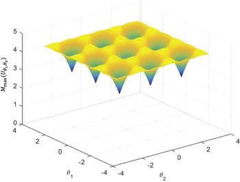
Figure 1. The graph of ${M}_{\max }({U}_{{\theta }_{1},{\theta }_{2}})$ on the domain θ1, θ2 ∈ [−π, π). We see that there are 18 pairs of (θ1, θ2) achieving the same maximal value $1+2\sqrt{3}\approx 4.4641.$ In the region −πθ1θ2 < π, there are 9 pairs of (θ1, θ2), as listed in table 3, which achieve the maximal value. We also observe that ${M}_{\max }({U}_{{\theta }_{1},{\theta }_{2}})\geqslant 3$.
Let (noting here ω = e2πi/3)
$\begin{eqnarray}S=| 0\rangle \langle 0| +| 1\rangle \langle 1| +\omega | 2\rangle \langle 2| =\left(\begin{array}{ccc}1 & 0 & 0\\ 0 & 1 & 0\\ 0 & 0 & \omega \end{array}\right)\end{eqnarray}$
be the qutrit phase gate, which is a Clifford unitary since SXS = XZ and SZS = Z. The following result shows that up to Clifford equivalence, the gate T3 is essentially the only gate among the diagonal unitary gates for optimally generating the magic resource: All the gates listed in table 3 are Clifford equivalent to the gate T3, i.e. are of the forms VT3W for some Clifford unitaries $V,W\in {{ \mathcal C }}_{3}.$ More explicitly

U−2π/9,2π/9 = T3,

U−4π/9,4π/9 = H2T3H2Z2,

U−8π/9,8π/9 = T3Z2,

U−8π/9,−4π/9 = T3Z2S,

U−8π/9,2π/9 = T3Z2S2,

U−4π/9,−2π/9 = H2T3H2Z2S2,

U−2π/9,8π/9 = T3S.

U2π/9,4π/9 = H2T3H2S,

U4π/9,8π/9 = T3ZS2.

Here H is the qutrit Hadamard gate defined by equation (8), and S is the qutrit phase gate defined by equation (12). The proof is via direct verification.
We emphasize that although in the gate set $\{{U}_{{\theta }_{1},{\theta }_{2}}:{\theta }_{1},{\theta }_{2}\in [-\pi ,\pi )\},$ the qutrit T-gate T3 has the maximal magic-resource-generating power, there exist non-diagonal gates possessing higher magic-resource-generating power since, for a qutrit system (d = 3)
$\begin{eqnarray*}\begin{array}{l}\mathop{\max }\limits_{\rho }M(\rho )=1+(3-1)\sqrt{3+1}\\ \quad =5\gt {M}_{\max }({T}_{3})=1+2\sqrt{3}.\end{array}\end{eqnarray*}$
For example, any unitary operator ${U}_{0}\in {{ \mathcal U }}_{3}$ satisfying
$\begin{eqnarray*}{U}_{0}| 0\rangle =\displaystyle \frac{1}{\sqrt{2}}(| 1\rangle -| 2\rangle )\end{eqnarray*}$
has the maximal magic-resource-generating power
$\begin{eqnarray*}{M}_{\max }({U}_{0})=\mathop{\max }\limits_{U\in {{ \mathcal U }}_{d}}{M}_{\max }(U)=5.\end{eqnarray*}$
We summarize the results in table 4.
Table 4. Comparison between magic-resource-generating power for diagonal and general (non-diagonal) unitary gates in qubit and qutrit systems. Here ${{ \mathcal D }}_{d}$ is the set of diagonal unitary operators, which is a subgroup of the set ${{ \mathcal U }}_{d}$ of all unitary operators.
d ${\max }_{U\in {{ \mathcal D }}_{d}}{M}_{\max }(U)={M}_{\max }({T}_{d})$ ${\max }_{U\in {{ \mathcal U }}_{d}}{M}_{\max }(U)$
2 (qubit) $1+\sqrt{2}$ $1+\sqrt{3}$
3 (qutrit) $1+2\sqrt{3}$ 5

4. Summary

In the stabilizer formalism of fault-tolerant quantum computation, the Clifford +T gate set is usually adapted as the basic structure. Since by the Gottesman–Knill theorem, the Clifford circuits can be efficiently simulated by classical means, the quantum power comes from the T-gate and its interaction with Clifford circuits. The T-gate is widely employed to generate magic resource (magic states) from stabilizer states. Consequently, it is desirable to study the power of the T-gate for generating magic resource, and to ask whether it is optimal in some sense.
By employing a natural quantifier of magic (non-stabilizerness), we have shown that the qubit T-gate and qutrit T-gate are indeed optimal for generating magic resource among the class of diagonal unitaries, and furthermore, up to Clifford equivalence, they are essentially the only ones. This highlights a fundamental and optimal feature of the T-gate, and provides new support for the utilization of the T-gate.
For higher dimensional systems, the calculation is considerably more complicated, and we may expect similar results. However, this calls for further investigations. It is certainly worthwhile to classify and identify the optimal gates for generating magic resource in the general case for other quantifiers of magic, such as the relative entropy of magic and sum negativity.

Appendix

Here we present the detailed proof of proposition 2 in section 3.

We first establish equation (10). For the qutrit stabilizer states listed in table 2, by direct calculations, we have

$\begin{eqnarray}M({U}_{{\theta }_{1},{\theta }_{2}}| {\phi }_{j}\rangle )=3,\qquad j=1,2,3\end{eqnarray}$
and
$\begin{eqnarray}M({U}_{{\theta }_{1},{\theta }_{2}}| {\phi }_{j}\rangle )=1+\displaystyle \frac{2}{3}\displaystyle \sum _{k=0}^{2}\sqrt{3+2{x}_{k}},\qquad j=4,\cdots ,12\end{eqnarray}$
with
$\begin{eqnarray*}\begin{array}{rcl}{x}_{k} & = & \cos \left(\alpha +\displaystyle \frac{2k\pi }{3}\right)+\cos \left(-\displaystyle \frac{\alpha }{2}+\displaystyle \frac{3\beta }{2}+\displaystyle \frac{2k\pi }{3}\right)\\ & & +\cos \left(-\displaystyle \frac{\alpha }{2}-\displaystyle \frac{3\beta }{2}+\displaystyle \frac{2k\pi }{3}\right),\qquad k=0,1,2,\end{array}\end{eqnarray*}$
and
$\begin{eqnarray*}\alpha ={\theta }_{1}+{\theta }_{2}\in [-2\pi ,2\pi ),\quad \beta ={\theta }_{1}-{\theta }_{2}\in (-2\pi ,0].\end{eqnarray*}$
Noting that
$\begin{eqnarray*}\displaystyle \sum _{k=0}^{2}\cos \left(x+\displaystyle \frac{2k\pi }{3}\right)=0,\qquad \forall \ x\in [0,2\pi ),\end{eqnarray*}$
we obtain
$\begin{eqnarray}\displaystyle \sum _{k=0}^{2}{x}_{k}=0.\end{eqnarray}$

We need to maximize the quantity

$\begin{eqnarray*}{M}_{\max }({U}_{{\theta }_{1},{\theta }_{2}})=1+\displaystyle \frac{2}{3}\displaystyle \sum _{k=0}^{2}\sqrt{3+2{x}_{k}}\end{eqnarray*}$
over the region −πθ1θ2 < π. By the Cauchy–Schwarz inequality, we have
$\begin{eqnarray*}{\left(\displaystyle \sum _{k=0}^{2}\sqrt{3+2{x}_{k}}\right)}^{2}\leqslant \left(\displaystyle \sum _{k=0}^{2}(3+2{x}_{k})\right)\left(\displaystyle \sum _{k=0}^{2}{1}^{2}\right)=27,\end{eqnarray*}$
with the equality holding if and only if
$\begin{eqnarray*}{x}_{0}={x}_{1}={x}_{2}.\end{eqnarray*}$
Combined with equation (A3), we have
$\begin{eqnarray*}{x}_{0}={x}_{1}={x}_{2}=0.\end{eqnarray*}$
From x0 = 0 we obtain
$\begin{eqnarray}\cos \ \alpha +\cos \left(-\displaystyle \frac{\alpha }{2}+\displaystyle \frac{3\beta }{2}\right)+\cos \left(-\displaystyle \frac{\alpha }{2}-\displaystyle \frac{3\beta }{2}\right)=0.\end{eqnarray}$
From x1 = 0 we obtain
$\begin{eqnarray*}\begin{array}{l}\left(\cos \ \alpha +\cos \left(-\displaystyle \frac{\alpha }{2}+\displaystyle \frac{3\beta }{2}\right)\right.\\ \quad \left.+\cos \left(-\displaystyle \frac{\alpha }{2}-\displaystyle \frac{3\beta }{2}\right)\right)\cos \displaystyle \frac{2\pi }{3}\\ \quad +\left(\sin \ \alpha +\sin \left(-\displaystyle \frac{\alpha }{2}+\displaystyle \frac{3\beta }{2}\right)\right.\\ \quad \left.+\sin \left(-\displaystyle \frac{\alpha }{2}-\displaystyle \frac{3\beta }{2}\right)\right)\sin \displaystyle \frac{2\pi }{3}=0.\end{array}\end{eqnarray*}$
Combined with equation (A4), we obtain
$\begin{eqnarray}\sin \ \alpha +\sin \left(-\displaystyle \frac{\alpha }{2}+\displaystyle \frac{3\beta }{2}\right)+\sin \left(-\displaystyle \frac{\alpha }{2}-\displaystyle \frac{3\beta }{2}\right)=0.\end{eqnarray}$

Now equations (A4) and (A5) can be equivalently rewritten as

$\begin{eqnarray}2\cos {}^{2}\displaystyle \frac{\alpha }{2}-1+2\cos \displaystyle \frac{\alpha }{2}\cos \displaystyle \frac{3\beta }{2}=0,\end{eqnarray}$
$\begin{eqnarray}2\sin \ \displaystyle \frac{\alpha }{2}\left(\cos \displaystyle \frac{\alpha }{2}-\cos \displaystyle \frac{3\beta }{2}\right)=0,\end{eqnarray}$
respectively. The solutions of equations (A6) and (A7) can be directly obtained by considering the following exhaustive cases:

i

(i) From equation (A7), we conclude that either $\sin \ \tfrac{\alpha }{2}=0$ or $\cos \tfrac{\alpha }{2}-\cos \tfrac{3\beta }{2}=0.$ First consider the case $\sin \ \tfrac{\alpha }{2}=0,$ then α = −2π, 0 (noting that α ∈ [−2π, 2π)). We have two subcases

a

(a) α = −2π, then θ1 = θ2 = −π and β = θ1θ2 = 0. This subcase is excluded by equation (A6) since it cannot be satisfied.

b

(b) α = 0, then $\cos \ \tfrac{\alpha }{2}=1,$ and by equation (A6), $\cos \ \tfrac{3\beta }{2}=-\tfrac{1}{2},$ which in turn implies that $\tfrac{3\beta }{2}=-\tfrac{2\pi }{3},-\tfrac{4\pi }{3},-\tfrac{8\pi }{3}$ (noting that β ∈ (−2π, 0]), that is,

$\begin{eqnarray*}\beta =-\displaystyle \frac{4\pi }{9},-\displaystyle \frac{8\pi }{9},-\displaystyle \frac{16\pi }{9}.\end{eqnarray*}$

Consequently, in this subcase, we obtain three solutions of equations (A6) and (A7) as

$\begin{eqnarray*}{\theta }_{1}=-{\theta }_{2}=-\displaystyle \frac{2\pi }{9},-\displaystyle \frac{4\pi }{9},-\displaystyle \frac{8\pi }{9}.\end{eqnarray*}$
In particular, the qutrit T-gate T3 corresponds to ${U}_{{\theta }_{1},{\theta }_{2}}$ with
$\begin{eqnarray*}{\theta }_{1}=-{\theta }_{2}=-\displaystyle \frac{2\pi }{9}.\end{eqnarray*}$
This establishes equation (10).

For clarity, we list the above optimal solutions in table A1.

i

(ii) Now consider the case $\cos \tfrac{\alpha }{2}-\cos \tfrac{3\beta }{2}=0,$ then combined with equation (A6), we have $\cos \tfrac{3\beta }{2}=\pm \tfrac{1}{2}.$ We have two subcases:

a

(a) $\cos \tfrac{3\beta }{2}=-\tfrac{1}{2}.$ In this subcase, $\cos \tfrac{\alpha }{2}=-\tfrac{1}{2}.$ Consequently, $\tfrac{3\beta }{2}=-\pi \pm \tfrac{\pi }{3},-3\pi +\tfrac{\pi }{3}$ (noting that β ∈ (−2π, 0]), i.e. $\beta =-\tfrac{4\pi }{9},-\tfrac{8\pi }{9},-\tfrac{16\pi }{9},$ and $\alpha =\pm \tfrac{4\pi }{3}$ (noting that α ∈ [−2π, 2π)). In this subcase, we obtain the optimal solutions as listed in table A2 (noting that we require θ1, θ2 ∈ [−π, π), θ1θ2).

b

(b) $\cos \tfrac{3\beta }{2}=\tfrac{1}{2}.$ In this subcase, $\cos \tfrac{\alpha }{2}=\tfrac{1}{2}.$ Consequently, $\tfrac{3\beta }{2}=-\tfrac{\pi }{3},-2\pi -\tfrac{\pi }{3},-2\pi +\tfrac{\pi }{3}$ (noting that β ∈ (−2π, 0]), i.e. $\beta =-\tfrac{2\pi }{9},-\tfrac{10\pi }{9},-\tfrac{14\pi }{9},$ and $\tfrac{\alpha }{2}=\pm \tfrac{\pi }{3}$ (noting that α ∈ [−2π, 2π)). In this subcase, we obtain the optimal solutions as listed in table A3 (noting that we require θ1, θ2 ∈ [−π, π), θ1θ2).

Table A1. Optimal solutions for the case (i).
θ1 $-\tfrac{2\pi }{9}$ $-\tfrac{4\pi }{9}$ $-\tfrac{8\pi }{9}$
θ2 $\tfrac{2\pi }{9}$ $\tfrac{4\pi }{9}$ $\tfrac{8\pi }{9}$
Table A2. Optimal solutions for the subcase (ii)(a).
θ1 $-\tfrac{8\pi }{9}$ $\tfrac{4\pi }{9}$
θ2 $-\tfrac{4\pi }{9}$ $\tfrac{8\pi }{9}$
Table A3. Optimal solutions for the subcase (ii)(b).
θ1 $-\tfrac{8\pi }{9}$ $-\tfrac{4\pi }{9}$ $-\tfrac{2\pi }{9}$ $\tfrac{2\pi }{9}$
θ2 $\tfrac{2\pi }{9}$ $-\tfrac{2\pi }{9}$ $\tfrac{8\pi }{9}$ $\tfrac{4\pi }{9}$

We list all solutions (θ1, θ2) of equations (A6) and (A7) achieving the maximal magic-resource-generating power in table 3 in section 3. The maximal value is

$\begin{eqnarray*}\mathop{\max }\limits_{{\theta }_{1},{\theta }_{2}}{M}_{\max }({U}_{{\theta }_{1},{\theta }_{2}})=1+\displaystyle \frac{2}{3}\sqrt{27}=1+2\sqrt{3}.\end{eqnarray*}$
From the above derivation, any gate ${U}_{{\theta }_{1},{\theta }_{2}}$ with (θ1, θ2) in table 3, as well as any of its Clifford equivalent, also has the maximal magic-resource-generating power, with the maximal value
$\begin{eqnarray*}\mathop{\max }\limits_{{\theta }_{1},{\theta }_{2}}{M}_{\max }({U}_{{\theta }_{1},{\theta }_{2}})={M}_{\max }({T}_{3})=1+2\sqrt{3}.\end{eqnarray*}$

Finally, equation (11) follows readily from equation (10) since from equations (A1) and (A2), we have

$\begin{eqnarray*}\begin{array}{rcl}{M}_{\mathrm{ave}}({U}_{{\theta }_{1},{\theta }_{2}}) & = & \displaystyle \frac{1}{12}\left(3\times 3+9\left(1+\displaystyle \frac{2}{3}\displaystyle \sum _{k=0}^{2}\sqrt{3+2{x}_{k}}\right)\right)\\ & = & \displaystyle \frac{3}{4}\left(1+{M}_{\max }({U}_{{\theta }_{1},{\theta }_{2}})\right),\end{array}\end{eqnarray*}$
which implies that the solutions of (θ1, θ2) for achieving the maximal value of ${M}_{\mathrm{ave}}({U}_{{\theta }_{1},{\theta }_{2}})$ are the same as those for ${M}_{\max }({U}_{{\theta }_{1},{\theta }_{2}})$.

This work was supported by the National Key R&D Program of China, Grant No. 2020YFA0712700, and the National Natural Science Foundation of China, Grant No. 11875317.

1
Gottesman D 1997 Stabilizer codes and quantum error correction Ph. D. Thesis California Institute of Technology

2
Gottesman D 1998 The Heisenberg representation of quantum computers arXiv:quant-ph/9807006

3
Gottesman D Chuang I 1999 Demonstrating the viability of universal quantum computation using teleportation and single-qubit operations Nature 402 390

DOI

4
Zhou X Leung D W Chuang I L 2000 Methodology for quantum logic gate construction Phys. Rev. A 62 052316

DOI

5
Aaronson S Gottesman D 2004 Improved simulation of stabilizer circuits Phys. Rev. A 70 052328

DOI

6
Bravyi S Kitaev A 2005 Universal quantum computation with ideal Clifford gates and noisy ancillas Phys. Rev. A 71 022316

DOI

7
Gross D 2006 Hudson's theorem for finite-dimensional quantum systems J. Math. Phys. 47 122107

DOI

8
Nielsen M A Chuang I L 2010 Quantum Computation and Quantum Information (Cambridge Cambridge University Press)

9
Anwar H Campbell E T Browne D E 2012 Qutrit magic state distillation New J. Phys. 14 063006

DOI

10
Campbell E T Anwar H Browne D E 2012 Magic-state distillation in all prime dimensions using quantum Reed–Muller codes Phys. Rev. X 2 041021

DOI

11
Veitch V Mousavian S A H Gottesman D Emerson J 2014 The resource theory of stabilizer quantum computation New J. Phys. 16 013009

DOI

12
Bravyi S Gosset D 2016 Improved classical simulation of quantum circuits dominated by Clifford gates Phys. Rev. Lett. 116 250501

DOI

13
Bravyi S Smith G Smolin J A 2016 Trading classical and quantum computational resources Phys. Rev. X 6 021043

DOI

14
Campbell E Howard M 2017 Unifying gate synthesis and magic state distillation Phys. Rev. Lett. 118 060501

DOI

15
Howard M Campbell E 2017 Application of a resource theory for magic states to fault-tolerant quantum computing Phys. Rev. Lett. 118 090501

DOI

16
Ahmadi M Dang H B Gour G Sanders B C 2018 Quantification and manipulation of magic states Phys. Rev. A 97 062332

DOI

17
Heinrich M Gross D 2019 Robustness of magic and symmetries of the stabiliser polytope Quantum 3 132

DOI

18
Bravyi S Browne D Calpin P Campbell E Gosset D Howard M 2019 Simulation of quantum circuits by low-rank stabilizer decompositions Quantum 3 181

DOI

19
Seddon J R Campbell E T 2019 Quantifying magic for multi-qubit operations Proc. Roy. Soc. A 475 103002

DOI

20
Wang X Wilde M M Su Y 2019 Quantifying the magic of quantum channels New J. Phys. 21 103002

DOI

21
Wang X Wilde M M Su Y 2020 Efficiently computable bounds for magic state distillation Phys. Rev. Lett. 124 090505

DOI

22
Dai H Fu S Luo S 2022 Detecting magic states via characteristic functions Int. J. Theor. Phys. 61 35

DOI

23
Howard M Vala J 2012 Qudit versions of the qubit π/8 gate Phys. Rev. A 86 022316

DOI

24
Giles B Selinger P 2013 Exact synthesis of multiqubit Clifford +T circuits Phys. Rev. A 87 032332

DOI

25
Gosset D Kliuchnikov V Mosca M Russo V 2013 An algorithm for the T-count arXiv:1308.4134v1

26
Selinger P 2014 Efficient Clifford +T approximation of single-qubit operators arXiv:1212.6253v2

27
Watson F H E Campbell E T Anwar H Browne D E 2015 Qudit color codes and gauge color codes in all spatial dimensions Phys. Rev. A 92 022312

DOI

28
Ross N J Selinger P 2016 Optimal ancilla-free Clifford +T approximation of z-rotations Quantum Inf. Comput. 16 901

DOI

29
Zhang F Chen J 2019 Optimizing T gates in Clifford +T circuit as π/4 rotations around Paulis arXiv:1903.12456v1

30
Amy M Glaudell A N Ross N J 2020 Number-theoretic characterizations of some restricted Clifford +T circuits arXiv:1908.06076v3

31
Glaudell A N Ross N J Taylor J M 2019 Canonical forms for single-qutrit Clifford+T operatorts Ann. Phys. 406 54

DOI

32
Giles B Selinger P 2019 Remarks on Matsumoto and Amano's normal form for single-qubit Clifford +T operators arXiv:1312.6584v2

33
Jiang J Wang X 2021 Lower bound the T-count via unitary stabilizer nullity arXiv:2103.09999v1

34
Glaudell A Ross N J van de Wetering J Yeh L 2022 Qutrit metaplectic gates are a subset of Clifford +T arXiv:2202.09235v2

35
Yeh L van de Wetering J 2022 Constructing all qutrit controlled Clifford +T gates in Clifford +T arXiv:2204.00552v1

36
Schwinger J 1960 Unitary operator bases Proc. Natl. Acad. Sci. USA 46 570

DOI

37
Zauner G 1999 Quantendesigns: Grundzüge einer nichtkommutativen Designtheorie PhD Thesis University of Vienna

For an English translation, see: Zauner G 2011 Quantum designs: foundations of a noncommutative design theory Int. J. Quantum Inf. 9 445

DOI

38
Renes J M Blume-Kohout R Scott A J Caves C M 2004 Symmetric informationally complete quantum measurements J. Math. Phys. 45 2171

DOI

39
Appleby D M 2005 Symmetric informationally complete-positive operator valued measures and the extended Clifford group J. Math. Phys. 46 052107

DOI

40
Scott A J 2006 Tight informationally complete quantum measurements J. Phys. A 39 13507

DOI

41
Flammia S T 2006 On SIC-POVMs in prime dimensions J. Phys. A 39 13483

DOI

42
Zhu H 2010 SIC POVMs and Clifford groups in prime dimensions J. Phys. A 43 305305

DOI

43
Scott A J Grassl M 2010 Symmetric informationally complete positive-operator-valued measures: a new computer study J. Math. Phys. 51 042203

DOI

44
Appleby D M Flammia S T Fuchs C A 2011 The Lie algebraic significance of symmetric informationally complete measurements J. Math. Phys. 52 022202

DOI

45
Appleby D M Fuchs C A Zhu H 2015 Group theoretic, Lie algebraic and Jordan algebraic formulations of the SIC existence problem Quantum Inf. Comput. 15 0061

DOI

46
Bengtsson I 2017 The number behind the simplest SIC-POVM Found. Phys. 47 1031

DOI

47
Scott A J 2017 SICs: extending the list of solutions arXiv:1703.03993

48
Grassl M Scott A J 2017 Fibonacci-Lucas SIC-POVMs J. Math. Phys. 58 122201

DOI

49
Fuchs C A Hoang M C Stacey B C 2017 The SIC question: history and state of play Axioms 6 21

DOI

50
Saraceno M Ermann L Cormick C 2017 Phase-space representations of symmetric informationally complete positive-operator-valued-measure fiducial states Phys. Rev. A 95 032102

DOI

51
Appleby M Chien T-Y Flammia S Waldron S 2018 Constructing exact symmetric informationally complete measurements from numerical solutions J. Phys. A 51 165302

DOI

52
Feng L Luo S 2022 Equioverlapping measurements Phys. Lett. A 445 128243

DOI

53
Feng L Luo S 2022 From stabilizer states to SIC-POVM fiducial states Theor. Math. Phys. 213 1747

DOI

Outlines

/