


1. Introduction
The resolution power of an imaging system is an important problem in optics [1, 2]. The conventional approach on measuring the resolution power is the Rayleigh criterion, which gives a minimum distance that two incoherent optical point sources can be distinguished in vision [3]. A modern approach on the resolution power can be established in terms of parameter estimation theory, where the resolution power is measured by the estimation precision of the separation between two optical point sources [4, 5]. By using quantum parameter estimation theory [6–8], which takes into consideration the optimization over quantum measurements, Tsang et al showed that the resolution power for two incoherent optical point sources in the sub-Rayleigh region can be grossly improved by the spatial mode demultiplexing (SPADE) measurement [9, 10].
The SPADE measurement is optimal for estimating the separation of two point sources but needs prior information about the centroid of the two point source to align the involved spatial modes [9]. On the other hand, direct imaging is good at estimating the centroid of two point sources but performs poorly for estimating the separation. The tradeoff between the measurement efficiencies for estimating the centroid and the separation is a manifestation of Heisenberg's uncertainty principle and can be analyzed by resorting to the information regret tradeoff relation (IRTR) [11].
The IRTR restricts the simultaneous optimization for the centroid estimation and the separation estimation through an incompatibility coefficient [12]. For a spatially-invariant imaging system with a Gaussian point-spread function, this incompatibility coefficient approaches to its maximum value as the separations go to zero and vanish for very large separations. Besides, the incompatibility coefficient has a nontrivial zero point when the separation is double the standard deviation of the intensity distribution, which we called the Rayleigh distance. This opens up the possibility of existing a measurement that is simultaneously optimal for estimating the centroid and the separation.
In this work, we will give a positive answer to the existence of a joint optimal measurement for estimating the centroid and the separation at the nontrivial zero point of the incompatibility coefficient. For quantum multiparameter estimation, a complete characterization of the condition on the existence of a measurement that is optimal for estimating all parameter remains open, e.g. see [13–15]. However, it is known that the eigenvectors of the symmetric logarithmic derivative (SLD) operator with respect to a parameter constitutes the basis of an optimal measurement for estimating that parameter [16]. The optimal measurement constructed in this way in general depends on the true value of the parameters to be estimated and thus cannot be directly applied when possible values of the parameters lie in a wide range [17]. Nevertheless, such an optimal measurement is still useful, as it reveals the fundamental limit of estimation precision and can be approached with adaptive feedback control [18, 19]. We will show that for the parameter estimation model of locating two incoherent optical point sources, the SLD operators with respect to the centroid and to the separation are both not unique. Although the 'standard' SLD operators considered in the previous work [9] are not commuting with each other, we can find another pair of commuting SLD operators at the nontrivial zero point of the incompatibility coefficient. Furthermore, we will construct a joint optimal measurement in terms of the common eigenvectors of the commuting SLD operators.
We organized this paper as follows. In section 2 , we give a brief introduction on quantum multiparameter estimation theory and the measurement incompatibility problem. In section 3 , we describe the necessary background about the joint estimation problem for locating two incoherent optical point sources. In section 4 , we investigate the joint optimal measurement for estimating both the centroid and the separation when the incompatibility coefficient vanishes. We summarize our work in section 5 .
2. Quantum multiparameter estimation theory
Let us start with a brief introduction on quantum multiparameter estimation and measurement incompatibility. Assume that the state of a quantum system depends on a set θ = (θ1, θ2, …, θn) of n unknown parameters and is described by a parametric family ρθ of density operator. The values of θ are estimated through processing the outcomes of a measurement performed on the quantum system. A quantum measurement can be mathematically described by a positive operator valued measure (POVM) M = {Ex∣Ex ≥ 0, ∑xEx = $I$}, where I denotes the identity operator and x the measurement outcomes. The probability of obtaining a measurement outcome x is $p(x)=\mathrm{tr}({\rho }_{\theta }{E}_{x})$ according to Born's rule in quantum mechanics. The data processing is represented by the estimators $\hat{\theta }=({\hat{\theta }}_{1},{\hat{\theta }}_{2},\ldots ,{\hat{\theta }}_{n})$, which are maps from the observation data to the estimates. The error-covariance matrix of any unbiased estimator obeys the Cramér–Rao bound [20, 21]
$\begin{eqnarray}\mathrm{Cov}(\hat{\theta })\geqslant {N}^{-1}F{\left(M\right)}^{-1},\end{eqnarray}$
where N is the number of experimental repetitions and F(M) is the Fisher information matrix (FIM) defined by $\begin{eqnarray}{[F(M)]}_{j,k}=\displaystyle \sum _{x}p{\left(x\right)}^{-1}\displaystyle \frac{\partial p(x)}{\partial {\theta }_{j}}\displaystyle \frac{\partial p(x)}{\partial {\theta }_{k}}.\end{eqnarray}$
The FIM depends on the quantum measurement, meaning that we can optimize over quantum measurements. In quantum estimation theory [16, 22–25], it is known that the FIM is bounded from above by the quantum FIM ${ \mathcal F }$ in the sense that $F(M)\leqslant { \mathcal F }$, i.e. ${ \mathcal F }-F(M)$ is positive semi-definite, for all POVMs M. The quantum FIM is defined by $\begin{eqnarray}{{ \mathcal F }}_{j,k}=\mathrm{Re}\,\mathrm{tr}({\rho }_{\theta }{L}_{j}{L}_{k}),\end{eqnarray}$
where the SLD operators Lj for θj are Hermitian operators satisfying $\begin{eqnarray}\displaystyle \frac{\partial {\rho }_{\theta }}{\partial {\theta }_{j}}=\displaystyle \frac{1}{2}({L}_{j}{\rho }_{\theta }+{\rho }_{\theta }{L}_{j}).\end{eqnarray}$
Note that the SLD operator might be not uniquely determined by the above equality; this fact will play an important role in our work.In general, the entries of the FIM cannot be simultaneously maximized by optimizing over quantum measurements; this is known as the measurement compatibility problem in quantum multiparameter estimation theory [14, 15, 26–28]. The degree of nonoptimality of a measurement for estimating an individual parameter θj can be measured by the square-rooted and normalized version of information regret [11]:6 ) holds. For mixed states, it remains open whether the IRTR is tight, even for the special case where the incompatibility coefficient cj,k vanishes.
$\begin{eqnarray}{{\rm{\Delta }}}_{j}={\left(\displaystyle \frac{{{ \mathcal F }}_{j,j}-{[F(M)]}_{j,j}}{{{ \mathcal F }}_{j,j}}\right)}^{1/2}.\end{eqnarray}$
As a manifestation of Heisenberg's uncertainty principle, the information regrets for any two different parameters, e.g. θj and θk, must obey the IRTR [11]: $\begin{eqnarray}{{\rm{\Delta }}}_{j}^{2}+{{\rm{\Delta }}}_{k}^{2}+2\sqrt{1-{c}_{j,k}^{2}}{{\rm{\Delta }}}_{j}{{\rm{\Delta }}}_{k}\geqslant {c}_{j,k}^{2},\end{eqnarray}$
where cj,k is the incompatibility coefficient defined as $\begin{eqnarray}{c}_{j,k}=\displaystyle \frac{\mathrm{tr}| \sqrt{\rho }[{L}_{j},{L}_{k}]\sqrt{\rho }| }{2\sqrt{{{ \mathcal F }}_{j,j}{{ \mathcal F }}_{k,k}}}\end{eqnarray}$
with $| X| := \sqrt{{X}^{\dagger }X}$ for any operator X. The IRTR is tight when ρ is pure, meaning that there always exists a quantum measurement such that the equality in equation (3. Estimation problem for locating two incoherent point sources
We now consider a concrete multiparameter estimation problem—the joint estimation of the centroid and the separation of two incoherent optical point sources [9]. The model is illustrated in figure 1. Following [9], the quantum states of the spatial degree of freedom of a photon arriving at the image plane can be described by the density operator
$\begin{eqnarray}\rho =\displaystyle \frac{1}{2}\left(\left|{\psi }_{1}\right\rangle \left\langle {\psi }_{1}\right|+\left|{\psi }_{2}\right\rangle \left\langle {\psi }_{2}\right|\right),\end{eqnarray}$
where $\left|{\psi }_{j}\right\rangle $ denotes the quantum state of a photon from the jth source. Denoted by ψ(x) the normalized point-spread function of the imaging sources. The state vector $\left|{\psi }_{j}\right\rangle $ can be expressed in the coordinate basis as $\begin{eqnarray}\left|{\psi }_{j}\right\rangle =\int {\rm{d}}x\,\psi (x-{X}_{j})\left|x\right\rangle ,\end{eqnarray}$
where $\left|x\right\rangle $ is the photon image-plane position eigenket. The parameters to be estimated are the centroid θ1 and the separation θ2 that are defined as $\begin{eqnarray}{\theta }_{1}=({X}_{1}+{X}_{2})/2\qquad \mathrm{and}\qquad {\theta }_{2}={X}_{2}-{X}_{1}.\end{eqnarray}$
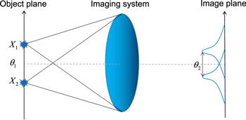
Figure 1. Model of resolving two incoherent optical point sources. Here, X1 and X2 are the one-dimensional coordinates of the first and second point sources, respectively. The parameters θ1 and θ2 represent the centroid and the separation of the two point sources, respectively. |
The SLD equation (4 ) can be solved by resorting to representing all relevant operators by a matrix with an orthonormal basis. A specific orthonormal basis for the minimal subspace that supports both ρ and its derivatives with respect to θ1 and θ2 is given by [9]7 ) is given by [12]:
$\begin{eqnarray}\begin{array}{rcl}\left|{e}_{1}\right\rangle & = & \displaystyle \frac{1}{\sqrt{2(1-\delta )}}\left(\left|{\psi }_{1}\right\rangle -\left|{\psi }_{2}\right\rangle \right),\\ \left|{e}_{2}\right\rangle & = & \displaystyle \frac{1}{\sqrt{2(1+\delta )}}\left(\left|{\psi }_{1}\right\rangle +\left|{\psi }_{2}\right\rangle \right),\\ \left|{e}_{3}\right\rangle & = & \displaystyle \frac{1}{{\eta }_{3}}\left[\displaystyle \frac{1}{\sqrt{2}}\left(\displaystyle \frac{\partial \left|{\psi }_{1}\right\rangle }{\partial {X}_{1}}+\displaystyle \frac{\partial \left|{\psi }_{2}\right\rangle }{\partial {X}_{2}}\right)-\displaystyle \frac{\gamma }{\sqrt{1-\delta }}\left|{e}_{1}\right\rangle \right],\\ \left|{e}_{4}\right\rangle & = & \displaystyle \frac{1}{{\eta }_{4}}\left[\displaystyle \frac{1}{\sqrt{2}}\left(\displaystyle \frac{\partial \left|{\psi }_{1}\right\rangle }{\partial {X}_{1}}-\displaystyle \frac{\partial \left|{\psi }_{2}\right\rangle }{\partial {X}_{2}}\right)+\displaystyle \frac{\gamma }{\sqrt{1+\delta }}\left|{e}_{2}\right\rangle \right],\end{array}\end{eqnarray}$
where the coefficients δ, κ, γ, and β are defined as $\begin{eqnarray}\begin{array}{rcl}\delta & = & \int {\rm{d}}x\,\psi (x-{X}_{1})\psi (x-{X}_{2}),\\ \kappa & = & {\int }_{-\infty }^{\infty }{\rm{d}}x{\left[\frac{\partial \psi (x)}{\partial x}\right]}^{2},\\ \gamma & = & {\int }_{-\infty }^{\infty }{\rm{d}}x\,\frac{\partial \psi (x)}{\partial x}\psi (x-{\theta }_{2}),\\ \beta & = & {\int }_{-\infty }^{\infty }{\rm{d}}x\,\frac{\partial \psi ({\rm{x}})}{\partial x}\frac{\partial \psi (x-{\theta }_{2})}{\partial x},\end{array}\end{eqnarray}$
and η3 and η4 are determined by the normalization condition as $\begin{eqnarray}{\eta }_{3}=\sqrt{\kappa +\beta -\displaystyle \frac{{\gamma }^{2}}{1-\delta }},\quad {\eta }_{4}=\sqrt{\kappa -\beta -\displaystyle \frac{{\gamma }^{2}}{1+\delta }}.\end{eqnarray}$
With this orthonormal basis, the density operator for the image-plane one-photon state is represented by $\begin{eqnarray}\rho =\displaystyle \frac{1-\delta }{2}\left|{e}_{1}\right\rangle \left\langle {e}_{1}\right|+\displaystyle \frac{1+\delta }{2}\left|{e}_{2}\right\rangle \left\langle {e}_{2}\right|.\end{eqnarray}$
The SLD operators with respect to θ1 and θ2 are represented by $\begin{eqnarray}\begin{array}{rcl}{L}_{1} & = & \left(\begin{array}{cccc}0 & \displaystyle \frac{2\gamma \delta }{\sqrt{1-{\delta }^{2}}} & 0 & \displaystyle \frac{2{\eta }_{4}}{\sqrt{1-\delta }}\\ \displaystyle \frac{2\gamma \delta }{\sqrt{1-{\delta }^{2}}} & 0 & \displaystyle \frac{2{\eta }_{3}}{\sqrt{1+\delta }} & 0\\ 0 & \displaystyle \frac{2{\eta }_{3}}{\sqrt{1+\delta }} & 0 & 0\\ \displaystyle \frac{2{\eta }_{4}}{\sqrt{1-\delta }} & 0 & 0 & 0\end{array}\right),\\ {L}_{2} & = & \left(\begin{array}{cccc}\displaystyle \frac{-\gamma }{1-\delta } & 0 & \displaystyle \frac{-{\eta }_{3}}{\sqrt{1-\delta }} & 0\\ 0 & \displaystyle \frac{\gamma }{1+\delta } & 0 & \displaystyle \frac{-{\eta }_{4}}{\sqrt{1+\delta }}\\ \displaystyle \frac{-{\eta }_{3}}{\sqrt{1-\delta }} & 0 & 0 & 0\\ 0 & \displaystyle \frac{-{\eta }_{4}}{\sqrt{1+\delta }} & 0 & 0\end{array}\right).\end{array}\end{eqnarray}$
With the above matrices, the incompatibility coefficient defined by equation ( $\begin{eqnarray}{c}^{2}=\displaystyle \frac{{\beta }^{2}}{\kappa (\kappa -{\gamma }^{2})}.\end{eqnarray}$
Here, we omit the subscripts of c for brevity, as we here only consider the estimation of two parameters.We are interested in the case where the incompatibility coefficient c becomes zero; This will happen when β vanishes according to equation (16 ). Assume that the point-spread function of the imaging system is Gaussian, viz.,
$\begin{eqnarray}\psi (x)={\left(2\pi {\sigma }^{2}\right)}^{-1/4}\exp \left(-\displaystyle \frac{{x}^{2}}{4{\sigma }^{2}}\right),\end{eqnarray}$
where σ is a characteristic width on the image plane. In such a case, it can be shown that [12] $\begin{eqnarray}\beta =\displaystyle \frac{4{\sigma }^{2}-{\theta }_{2}^{2}}{16{\sigma }^{2}}\exp \left(-\displaystyle \frac{{\theta }_{2}^{2}}{8{\sigma }^{2}}\right).\end{eqnarray}$
The nontrivial case of β = 0 occurs at θ2 = 2σ, which we call the Rayleigh distance. At this parameter point, the IRTR becomes ${{\rm{\Delta }}}_{1}^{2}+{{\rm{\Delta }}}_{2}^{2}\geqslant 0$, which no longer restricts the simultaneous optimization of quantum measurements for estimating the centroid and separation of two incoherent optical point sources. This gives us the possibility of an optimal joint measurement. If there exists such a measurement, it will outperform direct imaging and the SPADE measurement in the perspective of multiparameter estimation (see figure 2 for an illustration).
Figure 2. Information regrets for the centroid θ1 and the separation θ2 of direct imaging, the SPADE measurement, and the ideal optimal joint measurement. Here, the true value of the separation is set to θ2 = 2σ. The SPADE is performed with Hermite–Gaussian modes, whose origin point is placed at the centroid of the two sources. |
4. Joint optimal measurement
We now derive the joint optimal measurement for the aforementioned two-parameter estimation problem. Braunstein and Caves [16] showed that, for single parameter estimation, the POVM constituted by the eigen-projectors of the SLD operator is optimal in the sense that the extracted classical Fisher information attains its quantum limit—the quantum Fisher information. For multiparameter estimation, if the SLD operator commutes with each other, they have common eigen-projectors, which constitutes a joint optimal measurement in the sense that the classical FIM under this measurement equals to the quantum FIM. We will utilize this property to construct a joint optimal measurement for the problem of jointly estimating the centroid and separation of two incoherent optical point sources.
Although the SLD operators given in equation (15 ) do not commute with each other, it is possible to find a pair of commuting SLD operators, as the SLD operators might not be uniquely determined by an estimation problem. It is evident that, if Lj is an SLD operator of ρ with respect to θj and Kj is a Hermitian operator satisfying Kjρ = ρKj = 0, then ${L}_{j}^{\prime} \,={L}_{j}+{K}_{j}$ is also a Hermitian operator satisfying the SLD equation (4 ) and thus can be considered as an SLD operator. The additional Kj to the SLD operator does not affect the value of the quantum FIM as $\mathrm{tr}({L}_{j}\rho {L}_{k})=\mathrm{tr}[({L}_{j}+{K}_{j})\rho ({L}_{k}+{K}_{k})]$.
To find a set {Kj} of Hermitian operators such that the SLD operators commutes with each other, we will analyze in detail the representations of the SLD operator. Let ${ \mathcal H }$ be the (local) relevant Hilbert subspace of the estimation model at a parameter point θ. Concretely, ${ \mathcal H }$ is the union of the support of the density operators ρ and its derivatives ∂ρ/∂θj at the parameter point θ. Note that the relevant Hilbert subspace ${ \mathcal H }$ depends on the value of θ. We only need to consider the SLD operators acting on ${ \mathcal H }$. Furthermore, the Hilbert subspace can be decomposed as ${ \mathcal H }={ \mathcal S }\oplus { \mathcal K }$, where ${ \mathcal S }$ denotes the support of the density operator ρ and ${ \mathcal K }$ is the orthogonal complement of ${ \mathcal S }$ in ${ \mathcal H }$. We decompose the matrix representation of the SLD operators on ${ \mathcal H }$ in the block form with respect to the space decomposition ${ \mathcal H }={ \mathcal S }\oplus { \mathcal K }$:4 ), whereas Kj can be an arbitrary Hermitian matrix.
$\begin{eqnarray}{L}_{j}=\left(\begin{array}{cc}{A}_{j} & {B}_{j}\\ {B}_{j}^{\dagger } & {K}_{j}\end{array}\right).\end{eqnarray}$
Because Lj is Hermitian operators, the matrices Aj and Kj are all Hermitian. The matrices Aj and Bj are uniquely determined by the SLD equation (For the two-parameter estimation problem, we need to find the Hermitian matrices K1 and K2 such that L1L2 = L2L1. Using the above block forms, we get21 ) is a necessary condition on the existence of a joint optimal measurement. Equations (22 ) and (23 ) represent the conditions that should be satisfied by Kj.
$\begin{eqnarray}{L}_{1}{L}_{2}=\left(\begin{array}{cc}{A}_{1}{A}_{2}+{B}_{1}{B}_{2}^{\dagger } & {A}_{1}{B}_{2}+{B}_{1}{K}_{2}\\ {B}_{1}^{\dagger }{A}_{2}+{K}_{1}{B}_{2}^{\dagger } & {B}_{1}^{\dagger }{B}_{2}+{K}_{1}{K}_{2}\end{array}\right).\end{eqnarray}$
Comparing block by block both sides of the condition L1L2 = L2L1, we obtain the following equations: $\begin{eqnarray}{A}_{1}{A}_{2}-{A}_{2}{A}_{1}={B}_{2}{B}_{1}^{\dagger }-{B}_{1}{B}_{2}^{\dagger },\end{eqnarray}$
$\begin{eqnarray}{B}_{1}{K}_{2}-{B}_{2}{K}_{1}={A}_{2}{B}_{1}-{A}_{1}{B}_{2},\end{eqnarray}$
$\begin{eqnarray}{K}_{1}{K}_{2}-{K}_{2}{K}_{1}={B}_{2}^{\dagger }{B}_{1}-{B}_{1}^{\dagger }{B}_{2}.\end{eqnarray}$
Here, equation (For the concrete estimation problem considered in this paper, the set $\{\left|{e}_{j}\right\rangle | j=1,2,3,4\}$ given in equation (11 ) is an orthonormal basis of the relevant Hilbert subspace ${ \mathcal H }$. Meanwhile, the subspace ${ \mathcal S }$ and ${ \mathcal K }$ are spanned by $\{\left|{e}_{1}\right\rangle ,\left|{e}_{2}\right\rangle \}$ and $\{\left|{e}_{3}\right\rangle ,\left|{e}_{4}\right\rangle \}$, respectively. With this Hilbert space decomposition, we can extract the matrices A1, B1, A2, and B2 from the SLD operators given in equation (15 ). It can be verified that the necessary condition equation (21 ) is satisfied. For the canonical SLD operator in equation (15 ), both K1 and K2 are the zero matrix but can be set to arbitrary Hermitian matrices. Our objective is to find a pair of K1 and K2 that satisfy the conditions equations (22 ) and (23 ).
We can expand an arbitrary two-dimensional matrix X as the linear combination of the two-dimensional identity matrix ${\hat{\sigma }}_{0}$ and the Pauli matrices ${\hat{\sigma }}_{1}$, ${\hat{\sigma }}_{2}$, and ${\hat{\sigma }}_{3}$, namely,23 ) are traceless so that the expansion coefficients v0 of both sides vanish. Therefore, the conditions equation (22 ) and equation (23 ) give a system of 7 equations involving 8 variables, viz., vα(K1) and vα(K2) for α = 0, 1, 2, 3. This system of equations is undetermined and has infinitely many solutions. We give a specific solution as follows:
$\begin{eqnarray}X=\displaystyle \sum _{\alpha =0}^{3}{v}_{\alpha }(X){\hat{\sigma }}_{\alpha }\qquad \mathrm{with}\qquad {v}_{\alpha }(X)=\displaystyle \frac{1}{2}\mathrm{tr}({\hat{\sigma }}_{\alpha }X).\end{eqnarray}$
If X is Hermitian, vα(X) are all real numbers. Note that both sides of equation ( $\begin{eqnarray}{K}_{1}=\left(\displaystyle \frac{2\gamma }{1-{\delta }^{2}}-\displaystyle \frac{2\kappa }{\gamma }\right){\hat{\sigma }}_{0}-\displaystyle \frac{2\delta \gamma }{1-{\delta }^{2}}{\hat{\sigma }}_{3},\end{eqnarray}$
$\begin{eqnarray}{K}_{2}=\displaystyle \frac{{\eta }_{3}{\eta }_{4}}{\gamma }{\hat{\sigma }}_{1}+\displaystyle \frac{\left(1+{\delta }^{2}\right)\gamma }{1-{\delta }^{2}}{\hat{\sigma }}_{3}.\end{eqnarray}$
Putting the above K1 and K2 into equation (19 ), we get a pair of commuting SLD operators L1 and L2, which can be simultaneously diagonalized. Denote by φj the jth common eigenvectors of L1 and L2 and φj,k the kth component of φj. The measurement basis for the joint optimal measurement is given by11 ), we can express the wave function of the measurement basis $\left|{q}_{j}\right\rangle $ in terms of the point-spread function and its derivative. We numerically solve the common eigenvectors of L1 and L2 at the Rayleigh distance θ2 = 2σ and plot in figure 3 the wave function qj(x) = ⟨x∣qj⟩ of the joint optimal measurement basis.
$\begin{eqnarray}\left|{q}_{j}\right\rangle \equiv \displaystyle \sum _{k=1}^{4}{\phi }_{j,k}\left|{e}_{k}\right\rangle \qquad \mathrm{for}\qquad j=1,2,3,4.\end{eqnarray}$
With equation (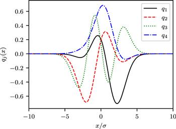
Figure 3. The wave functions of the measurement basis for the joint optimal measurement given in equation ( |
We here emphasize that the optimal measurement basis constructed by the eigenvectors of the SLD operator in general depends on the true values of the parameters to be estimated. The significance of such a measurement basis is that it can reveal the fundamental limit of the joint estimation precision with a quantum measurement. For practical application, the adaptive feedback control can help the quantum measurement approach to the optimal status.
5. Conclusions
In this work, we have constructed a joint optimal measurement that simultaneously extracts the maximal Fisher information about the centroid and the separation of two incoherent optical point sources. The method we used is utilizing the fact that the SLD operator is not uniquely determined by the parameter estimation model. By decomposing the SLD operators into the block form, we have found a pair of commuting SLD operators whose common eigenvectors can be taken as the basis of the joint optimal measurement. Our work, on the one hand, confirms the existence of a joint optimal measurement for the specific model of simultaneously estimating the centroid and the separation of two incoherent optical point sources at the Rayleigh distance, on the other hand, gives a promising method to characterize the condition on measurement compatibility for general multiparameter estimation problems.