


1. Introduction
The Kuramoto model is a paradigm for theoretically modeling collective behaviors in large systems of interacting agents. Since its introduction in 1975 [1], the model has been frequently used to explore synchronization transitions and relevant cooperative phenomena in numerous physical, biological, and social systems. Typical examples range from Josephson junctions [2], pacemaker cells in the heart [3], and power grids [4] to brain dynamics [5]. The model has attracted increasing interest in both physics and applied mathematics. Because it offers significant insights for a better understanding of synchronization transitions and various collective dynamics taking place in large populations of self-sustained oscillators [6–8].
The original version of the Kuramoto model elucidates synchronization transition emerging due to the interplay between the intrinsic frequency of the oscillators and the global coupling among them. Specifically, the heterogeneous natural frequencies distributed randomly according to a prescribed distribution tend to desynchronize the system, while the attracting coupling strength among the oscillators opposite this disorder tends towards synchrony [9–11].
In addition to the uniform coupling with a continuous phase transition, recent work in neuroscience and physics has highlighted the potential importance of the adaptive coupling between dynamical units. Namely, the coupling strength between individual oscillators is not necessarily uncorrelated, but rather oscillator dependent [12–14]. Such an adaptive scheme can be encoded by means of a nonlinear feedback function with respect to the global rhythm of the population. This adaptive rule often represents a realistic setup for a wide range of applications that goes beyond the conventional homogeneous coupling. For instance, such adaptive interactions have been used to describe the collective dynamics in neural networks with synaptic plasticity, or to describe the emergent behaviors in hypernetworks organized via nonpairwise (many body) interactions [15–19]. Despite substantial attention, the generic influence on the networked systems by the adaptive schemes remains largely unexplored.
In this work, we therefore consider a variant of the Kuramoto model incorporating the nonlinearity in the coupling. Specifically, we establish correlations between the coupling strength and the global rhythm of the population, in which the coupling is considered to be dependent on the amplitude of the mean field via a generic nonlinear function. As we will see, the interplay between these two effects significantly determines the overall collective behaviors as well as the local critical dynamics. More importantly, the model is analytically tractable, so our research provides theoretical insights for understanding the generic mechanism in coupled oscillator systems with adaptive coupling.
The aim of this paper is to provide a complete framework for investigating the generic dynamic properties induced by the nonlinear feedback function. To this end, we establish a self-consistent equation describing the order parameter that enables us to predict all possible equilibrium states of the system. Remarkably, we reveal that the property of the nonlinear function at its origin plays an important role in determining both the critical coupling and the types of the phase transition towards synchronization. Furthermore, we pay our particular attention to the relaxation dynamics of the incoherent state in the subcritical region by performing a detailed linear stability analysis. Correspondingly, the critical point characterizing the onset of synchronization is obtained analytically which is consistent with the analysis of the mean-field theory. The eigenspectrum structure of the linear operator demonstrates that the discrete spectrum is absent, manifesting a neutrally stable incoherent state. Nevertheless, we develop a framework for systematically exploring the relaxation dynamics of the equilibrium state in terms of the resonant pole theory. We show that the macroscopic order parameter does actually decay to zero in the long time limit, and the relaxation rate, which is due to analytic continuation, can be obtained from a general formula. All the theoretical results are well supported by the numerical simulations. In the following, we report both the theoretical and the numerical results in detail.
2. Dynamical model
We consider a generalized Kuramoto model, whose evolution is described by the following differential equations
$\begin{eqnarray}\dot{{\theta }_{i}}={\omega }_{i}+\displaystyle \frac{{Kf}(R)}{N}\displaystyle \sum _{j=1}^{N}\sin ({\theta }_{j}-{\theta }_{i}),i=1,...,N.\end{eqnarray}$
Here, θi(t) denotes the instantaneous phase of the ith oscillator. $\left\{{\omega }_{i}\right\}$ are the natural frequencies distributed according to a probability density g(ω). K > 0 is the coupling strength, and N is the size of the system. f(R) is a generic nonlinear function with respect to the amplitude of the order parameter defined by $\begin{eqnarray}Z(t)=R(t){{\rm{e}}}^{{\rm{i}}{\rm{\Theta }}(t)}=\displaystyle \frac{1}{N}\displaystyle \sum _{j=1}^{N}{{\rm{e}}}^{{\rm{i}}{\theta }_{j}(t)}.\end{eqnarray}$
Z(t) is the complex-valued vector within the unit circle representing the centroid of the configuration $\left\{{{\rm{e}}}^{{\rm{i}}{\theta }_{j}}\right\}$. R(t) and Θ(t) are respectively the amplitude and argument. Specifically, R(t) represents the level of the coherence of the system, and Θ(t) locates the average phase of the population. The most important feature of the model is that we introduce the adaptive coupling scheme [20, 21]. We emphasize that f(R) typically represents a sort of nonlinear correlation between the coupling and the global rhythm of the system, such as the synaptic plasticity of the neurons [22–24]. Depending on the intrinsic nonlinearity and the quenched disorder of the natural frequencies, the model defined above exhibits nontrivial collective behaviors, which are significantly richer than the dynamics of the traditional Kuramoto model with homogeneous linear coupling [25].Before proceeding with the analysis, we make a few remarks about the model. On the one hand, nonlinear coupling can be introduced by means of phase reduction in a system of limit cycle oscillators [26, 27]. For instance, one may set a power law function of f(R), i.e. f(R) = Rβ−1, with the exponent β > 1 and 0 < β ≤ 1, to establish the positive or the negative feedback between the coupling and the global coherence, respectively. On the other hand, recent works in neuroscience and physics highlighted the importance of high-order or group interactions, e.g. the interaction is described by three ways or more connections that are organized via simplicial complexes. More importantly, it has been shown that the effects of the high-order interactions are equivalent to the nonlinear coupling.
The aim of this work is to investigate the generic dynamical properties of the equilibrium states induced by nonlinear coupling. Without loss of generality, the distribution g(ω) is assumed to be unimodal and symmetric about the origin, i.e. g( − ω) = g(ω), and $g^{\prime} (\omega )\leqslant 0$ with ω ≥ 0. The function f(R) is an arbitrary nonlinear function of R, and f(R) > 0. These choices can be always achieved by rotating the frame and rescaling the time. Finally, the size N → ∞ is assumed throughout the paper.
3. Self-consistent approach
According to the definition of the order parameter equation (2 ) the governing equation (1 ) can be rewritten into the mean-field form as
$\begin{eqnarray}{\dot{\theta }}_{i}={\omega }_{i}+{Kf}(R)R\sin ({\rm{\Theta }}-{\theta }_{i}).\end{eqnarray}$
Remarkably, Kf(R)R represents an effective force acting on each individual phase oscillator.The next step is to formulate the self-consistent approach describing the stationary dynamics of equation (1 ). The key idea is to assume that the macroscopic quantity R(t) reaches a constant, and the average phase Θ(t) rotates uniformly in the long term evolution, i.e. Θ(t) = Ωt + Θ0. Furthermore, Θ0 and Ω can be set to zero by shifting initial conditions and setting up an appropriate rotating frame. Thus, equation (3 ) is simplified as
$\begin{eqnarray}{\dot{\theta }}_{i}={\omega }_{i}-{KRf}(R)\sin {\theta }_{i}.\end{eqnarray}$
Depending on the magnitude KRf(R), it can be seen from equation (4 ) that the phase oscillators exhibit two types of behaviors. Specifically, for $\left|{\omega }_{i}\right|\lt {KRf}(R)$, the oscillators are phase-locked with
$\begin{eqnarray}\sin {\theta }_{i}^{* }=\displaystyle \frac{{\omega }_{i}}{{KRf}(R)},\end{eqnarray}$
and $\begin{eqnarray}\cos {\theta }_{i}^{* }=\sqrt{1-\displaystyle \frac{{\omega }_{i}^{2}}{{K}^{2}{R}^{2}{f}^{2}(R)}}.\end{eqnarray}$
Correspondingly, in the limit N → ∞ , the distribution formed by the phase-locked oscillators is $\begin{eqnarray}{\rho }_{l}(\theta ,\omega )=\delta (\theta -{\theta }^{* }),\end{eqnarray}$
where δ( · ) denotes the Dirac function and the subscript l highlights the locked oscillators.When $\left|{\omega }_{i}\right|\gt {KRf}(R)$, the oscillators become drifting, i.e. they can never be entrained by the mean-field and rotate nonuniformly on the unit circle, thereby forming a smooth distribution given by
$\begin{eqnarray}{\rho }_{d}(\theta ,\omega )=\displaystyle \frac{\mathrm{sgn}(\omega )}{2\pi }\displaystyle \frac{\sqrt{{\omega }^{2}-{K}^{2}{R}^{2}{f}^{2}(R)}}{\omega -{KRf}(R)\sin \theta }.\end{eqnarray}$
Here $\mathrm{sgn}(\omega )$ is the sign function guaranteeing that the distribution is positive definite, and the subscript d highlights the drifting oscillators.The splitting of the population into the phase-locked cluster and the drifting cluster allows us to obtain the expression of the order parameter, which yields
$\begin{eqnarray}Z={\left\langle {{\rm{e}}}^{{\rm{i}}\theta }\right\rangle }_{l}+{\left\langle {{\rm{e}}}^{{\rm{i}}\theta }\right\rangle }_{d},\end{eqnarray}$
where $\left\langle \cdot \right\rangle $ denotes the average over the ensemble. A straightforward calculation shows that ${\left\langle {{\rm{e}}}^{{\rm{i}}\theta }\right\rangle }_{d}=0$, and ${\left\langle \sin \theta \right\rangle }_{l}=0$, which implies that the drifting population has no contribution to the order parameter and the locked ones only contribute to its real part. This symmetric condition is consistent with our previous assumption Θ = 0. Therefore, the order parameter is formulated as $\begin{eqnarray}R={\int }_{-{KRf}(R)}^{{KRf}(R)}\sqrt{1-\displaystyle \frac{{\omega }^{2}}{{K}^{2}{R}^{2}{f}^{2}(R)}}g(\omega ){\rm{d}}\omega .\end{eqnarray}$
Equation (10 ) provides a closed equation for the dependence of the amplitude R on the coupling strength K in terms of distribution g(ω) and the nonlinear coupling f(R). The expression for the order parameter R could be solved numerically or analytically for a given g(ω) and f(R). However, a full analysis of the stationary solution with an arbitrary form of g(ω) and any possible nonlinear function f(R) is beyond the scope of this research. Instead, we focus on the generic and representative properties of the self-consistent equation, for example, the critical point corresponding to the onset of synchronization.
First, we note that R = 0 is always a trivial solution of equation (10 ), which implies that the incoherent state always exists for any value of K and given f(R). The stability of this solution will be discussed in the following sections.
Apart from the trivial solution R = 0, let x = ω/KRf(R), the corresponding self-consistent equation is then reduced to the following form11 ), one obtains the critical coupling strength Kc yielding12 ) is a straightforward generalization of the result obtained by Kuramoto, in which f(R) = 1.
$\begin{eqnarray}\displaystyle \frac{1}{K}={\int }_{-1}^{1}\sqrt{1-{x}^{2}}g({KRf}(R)x)f(R){\rm{d}}x.\end{eqnarray}$
In the limit case R → 0+, taking into account the Taylor series expansion of the right-hand side of equation ( $\begin{eqnarray}{K}_{c}=\displaystyle \frac{2}{\pi g(0)f(0)}.\end{eqnarray}$
Obviously, equation (In light of the analysis above, the critical point characterizing the emergence of synchronization transition is determined by the value of the nonlinear function at its origin regardless of the specific form of f(R). In other words, the property of f(0) plays an essential role for the onset of synchrony, which can be discussed in three distinct scenarios. First, if f(0) is finite, then Kc is also finite. This demonstrates that the only effect of the nonlinear coupling is to delay or advance the threshold for the occurrence of synchronization. Second, if f(0) = 0, then Kc = +∞, which implies that the emergence of synchrony can never take place spontaneously. Third, if f(0) = +∞, then Kc = 0, which indicates that the transition to synchronization immediately occurs once K > 0.
The results above are summarized in figures 1–2. It should be pointed out that the analysis above does not depend on the specific form of g(ω) provided that it is a unimodal and symmetric one. To this end, in both panels, the distribution is $g(\omega )=\tfrac{1}{\sqrt{2\pi }}{{\rm{e}}}^{-\tfrac{{\omega }^{2}}{2}}$ (Gaussian distribution with unit width), and $f(R)={a}^{2}{{\rm{e}}}^{-{R}^{2}}$ (figure 1(a)), $f(R)=\tfrac{1}{{R}^{2}+{a}^{2}}$ (figure 1(b)). Figure 1 plots two typical cases of the critical coupling Kc as a function of the parameter a in the nonlinear function f(R), which exhibits a monotonously decreasing or increasing function of the parameter a, respectively.
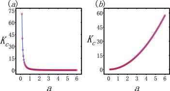
Figure 1. The critical coupling Kc versus the parameter a with $g(\omega )=\tfrac{1}{2\pi }{{\rm{e}}}^{-\tfrac{{\omega }^{2}}{2}}$. (a) $f(R)={a}^{2}{{\rm{e}}}^{-{R}^{2}}$. (b) $f(R)=\tfrac{1}{{R}^{2}+{a}^{2}}$. The solid lines are the theoretical predictions, and the circles are numerical simulations with N = 10 000. |
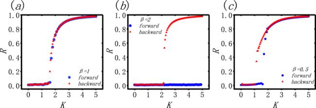
Figure 2. Phase diagram of the order parameter R versus the coupling strength K for different exponents β. The blue circles and the red triangles represent the forward and backward processes, respectively. The size N = 10 000. |
Figure 2 illustrates three different situations of phase transition toward synchronization. We set f(R) = Rβ−1. In figure 2(a), β = 1, which recovers the classical Kuramoto model. The system undergoes a second-order (continuous) phase transition to synchronization. In figure 2(b), β = 2, the corresponding feedback is weakened for 0 < R < 1. The system exhibits an irreversibly abrupt desynchronization transition, with the incoherent states being stable for the adiabatic forward processes. In contrast, the order parameter displays a continuous jump for the adiabatic backward continuations. In figure 2(c), β = 0.5, and the associated feedback is strengthened. The system experiences a phase transition to synchronization with the vanishing onset.
4. Linear stability analysis
The discussion above reveals that the mean-field theory provides a framework for characterizing the stationary behaviors and collective dynamics of the coupled system equation (1 ). Using the self-consistent equation, the collective amplitude R can be formally solved for the generic nonlinear function f(R). However, the stability properties of the equilibrium states are still unclear. In this section, we perform a detailed stability analysis to the incoherent state (R = 0). As it will appear momentarily, the spectrum structure of the incoherent state can be obtained analytically, which complements the self-consistent analysis.
In the thermodynamic limit N → ∞ , a probability density function ρ(θ, ω, t) can be used to characterize the microscopic dynamics. ρ(θ, ω, t)dθ accounts for the fraction of oscillators with phase lying in the interval (θ, θ + dθ) for a fixed time t and natural frequency ω. The normalization condition requires that2 ), which takes the integral form
$\begin{eqnarray}{\int }_{0}^{2\pi }\rho (\theta ,\omega ,t){\rm{d}}\theta =1.\end{eqnarray}$
Furthermore, the conservation of oscillator number implies a continuity equation of the form $\begin{eqnarray}\displaystyle \frac{\partial \rho }{\partial t}+\displaystyle \frac{\partial (\rho \upsilon )}{\partial \theta }=0.\end{eqnarray}$
The velocity field is given by $\begin{eqnarray}\upsilon =\omega +\displaystyle \frac{{Kf}(R)}{2i}(Z(t){{\rm{e}}}^{-{\rm{i}}\theta }-{Z}^{* }(t){{\rm{e}}}^{{\rm{i}}\theta }),\end{eqnarray}$
where Z(t) is the order parameter defined by equation ( $\begin{eqnarray}Z(t)={\int }_{-\infty }^{+\infty }{\int }_{0}^{2\pi }{{\rm{e}}}^{{\rm{i}}\theta }\rho (\theta ,\omega ,t)g(\omega ){\rm{d}}\theta {\rm{d}}\omega ,\end{eqnarray}$
and '*' denotes the complex conjugate.Notice that ρ(θ, ω, t) is a 2π-periodic function with respect to θ variable, which allows for a Fourier expansion of the form
$\begin{eqnarray}\rho (\theta ,\omega ,t)=\displaystyle \frac{1}{2\pi }\displaystyle \sum _{n=-\infty }^{+\infty }{z}_{n}(\omega ,t){{\rm{e}}}^{-{\rm{i}}n\theta }.\end{eqnarray}$
Here, zn(ω, t) is the nth Fourier coefficient defined by $\begin{eqnarray}{z}_{n}(\omega ,t)={\int }_{0}^{2\pi }{{\rm{e}}}^{{\rm{i}}n\theta }\rho (\theta ,\omega ,t){\rm{d}}\theta .\end{eqnarray}$
Obviously, z0 = 1 due to the normalization condition equation (13 ). Taking into account the real value of ρ(θ, ω, t), it can be shown that ${z}_{-n}={z}_{n}^{* }$. Substituting equation (17 ) into equation (14 ), the evolution of the Fourier coefficients satisfies the following differential equations
$\begin{eqnarray}\displaystyle \frac{{\rm{d}}{z}_{n}}{{\rm{d}}t}=n{\rm{i}}\omega {z}_{n}+\displaystyle \frac{{nKf}(R)}{2}(Z(t){z}_{n-1}-{Z}^{* }(t){z}_{n+1}),\end{eqnarray}$
which must be solved self-consistently with the order parameter given by $\begin{eqnarray}Z(t)={\int }_{-\infty }^{+\infty }{z}_{1}(\omega ,t)g(\omega ){\rm{d}}\omega =\hat{g}{z}_{1}(\omega ,t),\end{eqnarray}$
where the integral operator $\hat{g}$ is introduced to ease notation.It can be seen that equation (19 ) has a trivial fixed point zn = 0 with n ≠ 0, corresponding to the incoherent state $\rho (\theta ,\omega )=\tfrac{1}{2\pi }$, and R = 0. In order to study the stability of this steady state, we introduce small perturbations away from the incoherent state, i.e. zn(ω, t) = 0 + ϵηn(ω, t) (n ≠ 0) with 0 < ϵ ≪ 1 being the magnitude of the perturbation, and ηn(ω, t) is the perturbative vector. Correspondingly, the perturbed order parameter reads
$\begin{eqnarray}\varepsilon Z(t)=\varepsilon \hat{g}{\eta }_{l}(\omega ,t),\end{eqnarray}$
and the nonlinear function under perturbation becomes $\begin{eqnarray}\begin{array}{rcl}f(R) & = & f(\sqrt{{\varepsilon }^{2}Z(t){Z}^{* }(t)})\\ & = & f(\varepsilon \sqrt{\hat{g}{\eta }_{l}\hat{g}{\eta }_{l}^{* }})\\ & = & f(0)+\varepsilon f^{\prime} (0)\sqrt{\hat{g}{\eta }_{l}\hat{g}{\eta }_{l}^{* }}+O({\varepsilon }^{2}).\end{array}\end{eqnarray}$
Inserting these perturbations into equation (19 ) and ignoring the second and higher-order terms of ϵ, we get a set of linear evolution equations for ηn(ω, t), which are
$\begin{eqnarray}\displaystyle \frac{{\rm{d}}{\eta }_{l}}{{\rm{d}}t}={\rm{i}}\omega {\eta }_{l}+\displaystyle \frac{{Kf}(0)}{2}\hat{g}{\eta }_{l}={ \mathcal L }{\eta }_{l},\end{eqnarray}$
and $\begin{eqnarray}\displaystyle \frac{{\rm{d}}{\eta }_{n}}{{\rm{d}}t}=n{\rm{i}}\omega {\eta }_{n},\,n\gt 1.\end{eqnarray}$
The linear operator ${ \mathcal L }$ is defined as $\begin{eqnarray}{ \mathcal L }\phi (\omega )={\rm{i}}\omega \phi (\omega )+\displaystyle \frac{{Kf}(0)}{2}{\int }_{-\infty }^{+\infty }\phi (\omega )g(\omega ){\rm{d}}\omega ,\end{eqnarray}$
with φ(ω) being the smooth function.Regarding the high-order Fourier coefficient, we note from equation (24 ) that its solution has the form21 )). Hence, we only need to concentrate on the evolution of the l-th Fourier coefficient ηl(ω, t).
$\begin{eqnarray}{\eta }_{n}(\omega ,t)={{\rm{e}}}^{{\rm{i}}n\omega t}{\eta }_{n}(\omega ,0),\end{eqnarray}$
where ηn(ω, 0) represents its initial condition. This indicates that the magnitude of the perturbation remains unchanged under evolution, i.e. neutrally stable. At the same time, the high-order Fourier coefficient has no contribution to the order parameter itself (see equation (Let $\lambda \in {\mathbb{C}}$ be the eigenvalue of the linear operator ${ \mathcal L }$, we have28 ), we arrive at the self-consistent eigenvalue equation
$\begin{eqnarray}\displaystyle \frac{{\rm{d}}{\eta }_{l}}{{\rm{d}}t}={ \mathcal L }{\eta }_{l}=\lambda {\eta }_{l}.\end{eqnarray}$
Considering the definition of the operator ${ \mathcal L }$, we then obtain the vector $\begin{eqnarray}{\eta }_{l}=\displaystyle \frac{{Kf}(0)}{2}\displaystyle \frac{\hat{g}{\eta }_{l}}{\lambda -{\rm{i}}\omega }.\end{eqnarray}$
Applying the integral operator $\hat{g}$ to both sides of equation ( $\begin{eqnarray}\displaystyle \frac{1}{K}=\displaystyle \frac{f(0)}{2}\hat{g}\displaystyle \frac{1}{\lambda -{\rm{i}}\omega },\lambda \in {\mathbb{C}}\setminus {\rm{i}}\omega ,\end{eqnarray}$
where λ is on the complex plane except for those points $\left\{{\rm{i}}\omega \right\}$.Equation (29 ) relates implicitly the global coupling K with the eigenvalue λ. It has been proven that, for a unimodal distribution g(ω), $\lambda \in {\mathbb{R}}$. This conclusion coincides with the assumption Θ = 0, and the latter is closely related to the imaginary part of λ [28]. To simplify the discussion, we rewrite equation (29 ) into the following parametric form30 ) has only one positive root, which means that the incoherent state is linearly unstable. The critical case occurs at λ → 0+, at which the line K−1 is tangent to the curve F(λ) at its maximum. Accordingly, the critical point featuring the instability of the incoherent state is obtained by imposing the limit λ → 0+, which yields30 ) has no roots. Consequently, we conclude that the incoherent state is neutrally stable to perturbation in the subcritical region 0 < K < Kc, in which the linear operator ${ \mathcal L }$ has only the continuous spectrum $\left\{{\rm{i}}\omega \right\}$ lying on the whole imaginary axis.
$\begin{eqnarray}\displaystyle \frac{1}{K}=F(\lambda )=\displaystyle \frac{f(0)}{2}{\int }_{-\infty }^{+\infty }\displaystyle \frac{\lambda }{{\lambda }^{2}+{\omega }^{2}}g(\omega ){\rm{d}}\omega .\end{eqnarray}$
The sign of λ determines the stability of the incoherent state. It should be pointed out that λ > 0 provided that K > 0. Moreover, the parametric function F(λ) is strictly decreasing for λ > 0. To see this, $\begin{eqnarray}\begin{array}{rcl}\displaystyle \frac{{\rm{d}}F(\lambda )}{{\rm{d}}\lambda }\displaystyle \frac{1}{f(0)} & = & \displaystyle \frac{1}{2}{\int }_{-\infty }^{+\infty }\displaystyle \frac{{\omega }^{2}-{\lambda }^{2}}{{\left({\lambda }^{2}+{\omega }^{2}\right)}^{2}}g(\omega ){\rm{d}}\omega \\ & = & {\int }_{0}^{\lambda }\displaystyle \frac{{\omega }^{2}-{\lambda }^{2}}{{\left({\lambda }^{2}+{\omega }^{2}\right)}^{2}}g(\omega ){\rm{d}}\omega \\ & & +{\int }_{\lambda }^{+\infty }\displaystyle \frac{{\omega }^{2}-{\lambda }^{2}}{{\left({\lambda }^{2}+{\omega }^{2}\right)}^{2}}g(\omega ){\rm{d}}\omega \\ & \leqslant & g(\lambda ){\int }_{0}^{\lambda }\displaystyle \frac{{\omega }^{2}-{\lambda }^{2}}{{\left({\lambda }^{2}+{\omega }^{2}\right)}^{2}}{\rm{d}}\omega \\ & & +g(\lambda ){\int }_{\lambda }^{+\infty }\displaystyle \frac{{\omega }^{2}-{\lambda }^{2}}{{\left({\lambda }^{2}+{\omega }^{2}\right)}^{2}}{\rm{d}}\omega =0,\end{array}\end{eqnarray}$
and $\begin{eqnarray}\mathop{\mathrm{lim}}\limits_{\lambda \to +\infty }F(\lambda )=0,\end{eqnarray}$
as shown in figure 3. Therefore, for a sufficiently large value of K, equation ( $\begin{eqnarray}{K}_{c}=\mathop{\mathrm{lim}}\limits_{\lambda \to {0}^{+}}{F}^{-1}(\lambda )=\displaystyle \frac{2}{\pi g(0)f(0)}.\end{eqnarray}$
Once again, we recover the critical point for synchronization transition obtained by the self-consistent analysis. Furthermore, if the global coupling is decreased (K < Kc), the eigenvalue of the linear operator actually does not exist provided that f(0) > 0, since equation (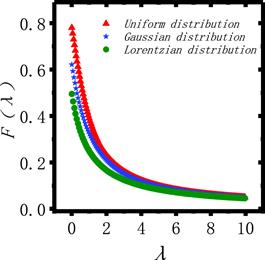
Figure 3. The schematic diagram of the parametric function F(λ) versus λ for different frequency distributions. |
It is worth mentioning that, for the limit case f(0) = 0, equation (30 ) has no roots for any value of K. Thus it can be confirmed that the incoherent state is always neutrally stable as long as K > 0, and the spontaneous transition to synchronization can never occur. On the contrary, for the case f(0) = +∞ , in which the nonlinear term dominates the coupling near R = 0, equation (30 ) must have at least one positive root. This implies that the incoherent state loses its stability so long as K > 0. As a result, in this scenario, the system undergoes a phase transition towards synchronization accompanied by the vanishing onset.
5. Relaxation dynamics of the incoherent state
Based on the discussion above, the microscopic incoherent state of the coupled system is only neutrally stable for K < Kc. However, it is well-known that the macroscopic order parameter actually decays to zero in an exponential form in the classical Kuramoto model, when the coupling strength is below the threshold for synchronization transition [29–31]. In this section, we show that such a decaying effect is far more generic even in such a system where the phase oscillators are coupled adaptively via a nonlinear feedback function.
Investigating such an issue may provide significant insights for understanding the intrinsic statistical mechanical properties of the equilibrium states. Since it has already been shown that the relaxation to the equilibrium is closely related to the susceptibility in response to external stimulations in statistical physics [32–34]. Remarkably, such a decaying mechanism is analogous to Landau damping in plasma physics [35–38]. To this end, we provide a general framework for determining the decaying exponents with extensive numerical simulations supporting the theoretical predictions as shown in figure 4.
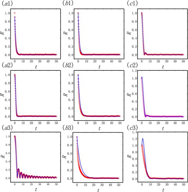
Figure 4. The perturbed order parameter R versus the time t for different control parameters Kf(0). The left column corresponds to Kf(0) = 0, with (a1) the Lorentzian distribution ${\left[\pi ({\omega }^{2}+1)\right]}^{-1}$, (a2) the Gaussian distribution $\tfrac{1}{\sqrt{2\pi }}{{\rm{e}}}^{-\tfrac{{\omega }^{2}}{2}}$, and (a3) the uniform distribution $g(\omega )=\tfrac{1}{2},\omega \in \left[-1,1\right]$. The middle column corresponds to ${\left[\pi ({\omega }^{2}+1)\right]}^{-1}$, with (b1) Kf(0) = 0.5, (b2) Kf(0) = 1.0, and (b3) Kf(0) = 1.5. The right column corresponds to $g(\omega )=\sqrt{2}{\left[\pi ({\omega }^{4}+1)\right]}^{-1}$, with (c1) Kf(0) = 0, (c2) Kf(0) = 0.5, and (c3) Kf(0) = 1.0. In all the panels, the solid lines are the theoretical predictions, and the circles are numerical simulations with N = 100 000. The initial value of each phase oscillator is set to be identical which implies that η1(ω, 0) ≡ 1. |
According to equation (23 ), a solution of the perturbation vector η1(ω, t) with an initial value η1(ω, 0) is formally solved as
$\begin{eqnarray}{\eta }_{1}(\omega ,t)={{\rm{e}}}^{{ \mathcal L }t}{\eta }_{1}(\omega ,0).\end{eqnarray}$
The operator ${e}^{{ \mathcal L }t}$ is calculated by means of the inverse Laplace transform, which yields $\begin{eqnarray}{{\rm{e}}}^{{ \mathcal L }t}=\displaystyle \frac{1}{2\pi {\rm{i}}}\mathop{\mathrm{lim}}\limits_{y\to +\infty }{\int }_{x-{\rm{i}}y}^{x+{\rm{i}}y}{{\rm{e}}}^{{st}}{\left(s-{ \mathcal L }\right)}^{-1}{\rm{d}}s,\end{eqnarray}$
for t > 0, and x > 0.Next, we focus on deriving the explicit expression of the resolvent ${\left(s-{ \mathcal L }\right)}^{-1}$. To do so, let φ(ω) be an arbitrary smooth function, we define36 ) by the operator $(s-{ \mathcal L })$, we thus have
$\begin{eqnarray}\begin{array}{rcl}{\boldsymbol{B}}(s)\phi (\omega ) & = & {\left(s-{ \mathcal L }\right)}^{-1}\phi (\omega )\\ & = & {\left(s-{\rm{i}}\omega -\displaystyle \frac{{Kf}(0)}{2}\hat{g}\right)}^{-1}\phi (\omega ).\end{array}\end{eqnarray}$
Multiplying both sides of the equation ( $\begin{eqnarray}\begin{array}{rcl}{\boldsymbol{B}}\left(s\right)\phi \left(\omega \right) & = & {\left(s-{\rm{i}}\omega \right)}^{-1}\phi \left(\omega \right)+\displaystyle \frac{{Kf}\left(0\right)}{2}{\left(s-{\rm{i}}\omega \right)}^{-1}\\ & & \times \,\hat{g}\left[{\boldsymbol{B}}(s)\phi (\omega )\right].\end{array}\end{eqnarray}$
Applying the integral operator $\hat{g}$ to both sides of equation (37 ), we obtain
$\begin{eqnarray}\hat{g}\left[{\boldsymbol{B}}(s)\phi (\omega )\right]=\hat{g}\left[\displaystyle \frac{\phi (\omega )}{s-{\rm{i}}\omega }\right]+\displaystyle \frac{{Kf}(0)}{2}\hat{g}\left[\displaystyle \frac{1}{s-{\rm{i}}\omega }\right]\hat{g}\left[{\boldsymbol{B}}(s)\phi (\omega )\right],\end{eqnarray}$
which is rearranged as $\begin{eqnarray}\hat{g}[{\boldsymbol{B}}(s)\phi (\omega )]=\displaystyle \frac{\hat{g}\left[\tfrac{\phi (\omega )}{s-{\rm{i}}\omega }\right]}{1-\tfrac{{Kf}(0)}{2}\hat{g}\left[\tfrac{1}{s-{\rm{i}}\omega }\right]}.\end{eqnarray}$
Turning to the order parameter, according to equation (20 ), equation (34 ), and equation (39 ), we have
$\begin{eqnarray}\begin{array}{rcl}Z(t) & = & \hat{g}{\eta }_{1}(\omega ,t)\\ & = & \hat{g}[{{\rm{e}}}^{{ \mathcal L }t}{\eta }_{1}(\omega ,0)]\\ & = & \displaystyle \frac{1}{2\pi {\rm{i}}}\mathop{\mathrm{lim}}\limits_{y\to +\infty }{\int }_{x-{\rm{i}}y}^{x+{\rm{i}}y}{{\rm{e}}}^{{st}}\hat{g}[{\left(s-{ \mathcal L }\right)}^{-1}{\eta }_{1}(\omega ,0)]{\rm{d}}s\\ & = & \displaystyle \frac{1}{2\pi {\rm{i}}}\mathop{\mathrm{lim}}\limits_{y\to +\infty }{\int }_{x-{\rm{i}}y}^{x+{\rm{i}}y}{{\rm{e}}}^{{st}}\hat{g}[{\boldsymbol{B}}(s){\eta }_{1}(\omega ,0)]{\rm{d}}s\\ & = & {{\boldsymbol{L}}}^{-1}[\displaystyle \frac{D(s)}{1-Q(s)}].\end{array}\end{eqnarray}$
L−1 denotes the inverse Laplace transform, and the two functions appearing in the numerator and denominator are given by $\begin{eqnarray}D(s)={\int }_{-\infty }^{+\infty }\displaystyle \frac{g(\omega ){\eta }_{1}(\omega ,0)}{s-{\rm{i}}\omega }{\rm{d}}\omega ,\end{eqnarray}$
and $\begin{eqnarray}Q(s)=\displaystyle \frac{{Kf}(0)}{2}{\int }_{-\infty }^{+\infty }\displaystyle \frac{g(\omega )}{s-{\rm{i}}\omega }{\rm{d}}\omega .\end{eqnarray}$
The inverse Laplace transform equation (40 ) is controlled by the poles of $\tfrac{D(s)}{1-Q(s)}$, which are exactly the resonant poles leading the order parameter to decay exponentially. To invert the Laplace transform, the calculation should be analytically continued to the left-half complex plane, where $\mathrm{Re}$(s) < 0. Indeed, if f(0) = 0, then the order parameter $Z(t)={{\boldsymbol{L}}}^{-1}[D(s)]=\hat{g}[{{\rm{e}}}^{{\rm{i}}\omega t}{\eta }_{1}(\omega ,0)]$, which is precisely the Fourier transform of g(ω)η1(ω, 0). Equivalently, each oscillator rotates at its own angular frequency provided that η1(ω, 0) is a constant. In fact, Z(t) → 0 in the long time limit t → ∞, which can be proven rigorously in terms of the Riemann-Lebesgue lemma. Namely, the order parameter of the incoherent state always relaxes to zero no matter how strong the coupling K is.
For the case f(0) = +∞, the resonant pole s0 determined from the identity 1 − Q(s) = 0 is equivalent to ${P}_{n}({s}_{0})=\tfrac{{Kf}(0)}{2}$, where Pn(s0) is the nth polynomial. This implies a positive root s0 once K > 0, causing the incoherent state to become unstable.
Lastly, if 0 < f(0) < + ∞ , and the distribution g(ω) is a rational case, e.g. ${g}_{n}(\omega )=\tfrac{n\sin (\tfrac{\pi }{2n})}{\pi ({\omega }^{2n}+1)}$ (the generalized Lorentzian distribution). The resonant poles can be calculated analytically For example, n = 1, we have ${s}_{0}=\tfrac{{Kf}(0)}{2}-1$. If n = 2, we have two resonant poles ${s}_{0,\pm }\,=\tfrac{1}{4}(-2\sqrt{2}+{Kf}(0)\pm \sqrt{-8\,+\,4\sqrt{2}{Kf}(0)+{K}^{2}{f}^{2}(0)})$. The above results suggest that the Landau damping effect is a generic property, which is rooted in the occurrence of the resonant poles caused by the analytic continuation. In the critical case $K\to \tfrac{2}{\pi g(0)f(0)}$, one of the resonant poles goes through the imaginary axis from left to right symbolizing the instability of an incoherent state.
The results are summarized in figure 4 where the numerical simulations confirm the theoretical predictions well except for a deviation at the beginning of time (figure 4(c)). Theoretically, it should be pointed out that the relaxation dynamics of the macroscopic order parameters are valid only in the linear region. It implies that the corresponding microscopic perturbed distribution should be near the incoherent state. In other words, the analytical expression for the time-varying order parameter (see equation (40 )) is asymptotically valid. This is because all the discussions about the relaxation dynamics are based on the framework of the linear stability analysis. Numerically, the initial phases of the oscillators are chosen to be identical to obtain the explicit formula of the order parameter. However, this initial perturbation is far away from the linear region. Nevertheless, the associated perturbation is getting closer and closer to the linear region with the evolution of time. Consequently, the corresponding deviation between the theoretical predictions and the numerical simulations will be smaller and smaller. This explains why there exists a deviation between the theory and the simulation during the initial transient time. Particularly, this feature becomes more evident when Kf(0) is slightly larger than zero.
6. Conclusions
To summarize, we extended the classical Kuramoto model for synchronization transition, occurring in the large populations of globally coupled phase oscillators, to an adaptively interacting coupling, where the homogeneous coupling strength is weighted by the global coherence of the system via a generic nonlinear function f(R). Theoretically, the mean-field theory, the linear stability analysis, and the resonant pole method have been carried out to get analytical insights. Together with the extensive numerical simulations, our research presented the following main results.
First, we formulated the self-consistent equation that describes the stationary behaviors of the system. Second, the analytical expression of the critical coupling characterizing the emergence of synchronization was established in a universal formula, where the property of the nonlinear function at its origin plays a crucial role in determining the critical coupling Kc as well as the ways of synchronization transition. Specifically, for a finite value of f(0), the threshold for phase transition is either postponed or accelerated. If f(0) = 0, an irreversibly abrupt desynchronization transition is identified. However, for the case f(0) = +∞ , the system undergoes a continuous phase transition with the vanishing onset. Third, the relaxation dynamics of the incoherent state were further addressed. We provided evidence of the subcritical region(K < Kc), in which the microscopic distribution is predicted to be neutrally stable to perturbation, while the macroscopic order parameter does decay exponentially. Furthermore, we developed a general framework for analytically determining the relaxation rate in terms of the resonant pole theory.
Our work provided a complete framework for investigating the generic dynamical properties of the phase oscillator models with nonlinear coupling, and the results could enhance our understanding of synchronization transition and collective dynamics in networked oscillators with adaptive coupling schemes.