


1. Introduction
At present, information storage and retrieval have become important functions of new magnetic materials. With the development of nanotechnology, the successful preparation of graphene and the excellent physical properties of graphene-like films in information storage have aroused significant interest from scientists [1–3]. On one hand, the graphene-like layers can display the magnetic characteristic by using physical and chemical methods, such as doping [4], adsorption [5], hydrogenation [6], and so on. On the other hand, the magnetic characteristics of the graphene-like layers structures are researched by many theoretical methods, such as effective field theory (EFT) [7], mean field theory [8], and density functional theory [9].
The Monte Carlo method, as one of the important methods, has been used to examine the magnetic properties of some graphene-like layered structures. In addition, the Ising model is a classical model to study the phase transition of various magnetic systems [10–12]. It is also worth noting that in order to reveal the interesting magnetic behaviors of Ising systems with graphene layers, a number of Monte Carlo researches have been employed. For example, the phase diagrams of the graphene monolayer were discussed [13]. Aktas et al researched the influence of thickness on magnetic behaviors in graphene-like layers [14]. R. Masrour et al revealed the significant role of defects on magnetization in the nano-graphene bilayer by using the Monte Carlo method [15]. Furthermore, the same method can also be employed to research the thermodynamic characteristics of the graphene-like bilayer caused by the magnetic field [16]. A number of novel magnetic behaviors have been observed. For instance, A. Mhirech expounded on the compensation behaviors of the graphene bilayer structure [17]. And the compensation behavior of the mixed spin-1 and spin-3/2 (1, 3/2) trilayer graphene structure was also investigated [18]. Besides the appearance of the compensation behavior, researchers focused more on the hysteresis behavior of the graphene-like layers. Magnetic properties of the bilayer-decorated graphene structure were investigated by N. Tahiri et al and they found that the exchange coupling can increase the value of the coercivity [19]. A. Jabar et al also obtained the triple hysteresis loops in the graphene with alternate layers [20]. It was found that not only the exchange coupling but also the temperature can affect the coercivity. The abundant magnetic behaviors of graphene-like layers such as the compensation behaviors and multiple hysteresis loops all arise our great interest.
Although many studies on the magnetic characteristics of graphene-like layers have been reported, little effort was made to clarify the phase diagrams and hysteresis behaviors in the graphene bilayer. What characteristics can the compensation behavior of this system display caused by crystal field and exchange coupling? In previous studies, we have presented the microscopic magnetic behavior of other nanostructures [21–33]. Accordingly, the paper aims to examine compensation temperature and hysteresis behaviors of a graphene-like bilayer, which is organized as follows: in section 2 , the Ising model and MC method are clarified. In section 3 , the magnetic behaviors of the system are discussed in detail. Finally, in section 4 , we give a brief conclusion.
2. Model and method
Figure 1 shows a ferrimagnetic mixed-spin (3/2, 5/2) Ising model on the graphene-like bilayer, which is composed of the spin-3/2 sublattices, a (red balls), and the spin-5/2 sublattices, b (blue balls). There are 2 × N2 × L spins on the graphene-like bilayer, where 2 × N2 is the number of spins per layer and L = 2 is the thickness of the bilayer. To determine the value of 2 × N2, we have increased the value of 2 × N2 from 2 × 202 to 2 × 602 for simulation. However, no obvious difference can be observed in this simulation. Hence, the size of graphene-like bilayer 2 × N2 × L = 2 × 202 × 2 was chosen for our simulation.
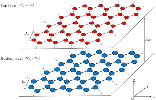
Figure 1. Three-dimensional view of the ferrimagnetic mixed-spin (3/2, 5/2) Ising model with the graphene-like bilayer. |
The Hamiltonian of this system is given as follows:
$\begin{eqnarray}\begin{array}{rcl}H & = & -{J}_{a}\displaystyle \sum _{\langle i,j\rangle }{\sigma }_{{ia}}^{z}{\sigma }_{{ja}}^{z}-{J}_{b}\displaystyle \sum _{\langle i^{\prime} ,j^{\prime} \rangle }{S}_{i^{\prime} a}^{z}{S}_{j^{\prime} a}^{z}\\ & & -{J}_{{ab}}\displaystyle \sum _{\langle i,i^{\prime} \rangle }{\sigma }_{{ia}}^{z}{S}_{i^{\prime} b}^{z}-{D}_{a}\displaystyle \sum _{\langle i\rangle }{\left({\sigma }_{{ia}}^{z}\right)}^{2}\\ & & -{D}_{b}\displaystyle \sum _{\langle i^{\prime} \rangle }{\left({S}_{i^{\prime} b}^{z}\right)}^{2}-h(\displaystyle \sum _{\langle i\rangle }{\sigma }_{{ia}}^{z}+\displaystyle \sum _{\langle i^{\prime} \rangle }{S}_{i^{\prime} b}^{z}),\end{array}\end{eqnarray}$
where, the spins of sublattices a and b take ${\sigma }_{{ia}}^{z}\,=\pm 3/2,\pm 1/2$ and ${S}_{{ja}}^{z}=\pm 5/2,\pm 3/2,\pm 1/2$, respectively. Ja and Jb represent the intralayer coupling between the same kind of sublattices a − a and b − b within the top and bottom layers, while Jab is the interlayer exchange coupling between sublattices a and b. Ja is chosen as the unit of energy and temperature and then is fixed 1. Da and Db are the crystal fields of sublattices a and b. Finally, the applied magnetic field is expressed by h.We used the Monte Carlo method described by the Metropolis algorithm [34] to simulate the ferrimagnetic bilayer. We employed periodic boundary conditions in the x and y directions, and the free boundary condition in the z direction. In addition, in order to balance this system, we discarded the first 3 × 10⁴ MC steps and used the remaining 5 × 10⁴ MC steps to obtain the simulation data. At last, the error bars were calculated through ten samples based on the Jackknife statistical approach [35]. The thermodynamic quantities are calculated as follows:
The internal energy of the system per spin is:
$\begin{eqnarray}U=\displaystyle \frac{1}{2{N}^{2}L}\langle H\rangle ,\end{eqnarray}$
The magnetic specific heat of the system per spin is given by: $\begin{eqnarray}\displaystyle \frac{C}{{k}_{{\rm{B}}}}=\displaystyle \frac{{\beta }^{2}}{2{N}^{2}L}(\langle {H}^{2}\rangle -\langle H{\rangle }^{2}).\end{eqnarray}$
The magnetizations of sublattices a and b per spin are presented by: $\begin{eqnarray}{M}_{a}=\displaystyle \frac{1}{2{N}^{2}}\displaystyle \sum _{i}{\sigma }_{{ia}}^{z},\end{eqnarray}$
$\begin{eqnarray}{M}_{b}=\displaystyle \frac{1}{2{N}^{2}}\displaystyle \sum _{j}{S}_{{jb}}^{z},\end{eqnarray}$
and the magnetization of the whole system per spin can be given by: $\begin{eqnarray}M=\displaystyle \frac{1}{2}({M}_{a}+{M}_{b}).\end{eqnarray}$
The susceptibilities of sublattices a and b per spin are described by: $\begin{eqnarray}{\chi }_{a}=2{N}^{2}\beta (\langle {M}_{a}^{2}\rangle -\langle {M}_{a}{\rangle }^{2}),\end{eqnarray}$
$\begin{eqnarray}{\chi }_{b}=2{N}^{2}\beta (\langle {M}_{b}^{2}\rangle -\langle {M}_{b}{\rangle }^{2}),\end{eqnarray}$
and the susceptibility of the whole system per spin is expressed by: $\begin{eqnarray}\chi =\displaystyle \frac{1}{2}({\chi }_{a}+{\chi }_{b}).\end{eqnarray}$
Here $\beta =\tfrac{1}{{k}_{{\rm{B}}}T}$, in which kB and T represent Boltzmann constant and temperature, respectively. Here, kB is set 1 for brevity.3. Results and discussion
3.1. Magnetization, susceptibility
Figures 2(a)–(c) show the effect of Da on the M, Ma, Mb, and χ with fixed Db = −0.4, Jab = −0.2, and Jb = −0.2. The different behaviors of M curves can be obviously noticed in figure 2(a). When Da is changed from −0.3 to −1.1, the M curves first begin from the same saturation value M = 0.5 to drop below zero and then approach the constant value (M = 0) with T increasing. It can be clearly noticed that there are two zero points in the M curves. The temperature corresponding to M = 0 in the low-temperature zone is the compensation temperature Tcomp, which can be widely applied in the magnetic recording device [36]. This type of M curve pertains to the N-type curves predicted by $N\acute{e}{el}$ theory [37]. For the above compensation behavior, an explanation can be given. As T increases, the Ma and Mb decrease at different speeds. Therefore, the Ma and Mb offset each other at the same temperature, at which total magnetization (M) is zero, known as the compensation temperature (Tcomp). In addition, as Da decreases, Tcomp moves slowly to the high-temperature zone. The stronger crystal field breaks the structural stability and makes the spins of sublattices flip more easily. In experiments, the compensation behavior has also been found in graphene-based film [38]. It has been found that the possibility of designing a magnetically compensated graphene-based SAF/SFiM system is based on the discovery of the compensation temperature. It is worth noting that Ju. A. Mamalui et al have found that the anisotropy in ferrite-garnet can influence the compensation temperature Tcomp of the system [39]. This is consistent with the conclusion found in figure 2(a). We can observe clearly in figure 2(b) that the magnetizations of sublattices (Ma, Mb) at Tcomp are equal in value and opposite in direction. When Da continues to be changed from −1.5 to −2.7, the P-type curves predicted by $N\acute{e}{el}$ theory [37] can be found. On one hand, the stronger Da can help the spins of the sublattice flip from the high spin state to the low one, resulting in the appearance of more spin configurations. We can also notice clearly in figure 2(b) that when Da = −2.7, Ma is changed from −1.5 to −0.5, and Mb is changed from 2.5 to 1.5. In fact, each kind of sublattice has its own crystal field, which affects the corresponding magnetization of the sublattice directly. For example, in figure 2(b), the crystal field of sublattice a Da can directly influence its magnetization Ma and correspondingly the saturation values of Ma are also changed. However, due to the existence of the exchange coupling Jab between the sublattices a and b, Mb is also affected by the change of Da. As one can notice, the Mb also exhibits an additional small saturation value Mb = 1.5 for the relatively strong anisotropy Da = −2.7. Besides, the profile of the Mb curve is not only directly determined by the crystal field Db, but also by the various exchange couplings Jab, Jb, and temperature. On the other hand, with the increase of temperature, the thermal disturbance can release the frustrated spin states, resulting in a significant reduction in the M with T increasing. Similarly, the same spin frustration behavior with the maximum of magnetic moment can be discovered in the experimental investigations of the graphene-layered structures [40, 41]. Namely, a maximum in the magnetization curve at low temperatures can be observed, which corresponds to the coexistence of the spins with different spin states. The effects of Da and T on susceptibility χ can be studied in figure 2(c). There is a peak in every χ curve corresponding to the transition temperature TC. It can be observed that the TC moves to the low-temperature zone as $\left|{D}_{a}\right|$ increases. This phenomenon is due to the competition between Da and T. The thermal disturbance caused by temperature increases the order of the system, while the negative increase of Da can make the system more disordered. In addition, when Da = −2.7, there are two peaks in the χ curve. The existence of a peak at low temperature should be associated with the sudden drop in the M curve with the same parameter in figure 2(a).
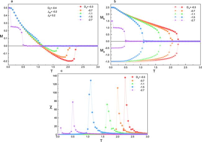
Figure 2. The influence of Da on the M, Ma, Mb, χ with fixed Db = −0.4, Jab = −0.2, and Jb = 0.2. |
Figures 3(a)–(c) show the impact of Db on M, Ma, Mb, and χ with fixed Da = −0.1, Jab = −0.2, Jb = 0.2. It can be found from figure 3(a) that compared with the effect of Da, the saturation values of M are sensitive to the effect of Db because the more saturation values of M(= 0.5, 0, −0.5) can be found. That is explained by the fact that there are more saturated spin values of sublattice b than those of sublattice a. We can notice in figure 3(b) that when Db is changed from −0.2 to −2.8, the saturation values of Mb are equal to 2.5, 1.5, and 0.5. Furthermore, when Db = −0.1 and −0.2, the N-type curves can be discovered. From figure 3(c), it can be found that the influence of Db on TC is similar to that of Da on TC. With $\left|{D}_{b}\right|$ increasing, the peak of the χ curve shifts to low temperature. Figures 4(a)–(c) present the temperature dependence of M, Ma, Mb, and χ for Jab with fixed Da = −0.1, Db = −0.4, Jb = 0.2. It can be obviously observed from figure 5(a) that two saturation values (M = 0, 0.5) are found caused by Jab. This can also be reflected in figure 4(b). With the increase of Jab, the saturation values of Mb are changed from 2.5 to 1.5, while the saturation value of Ma is not changed. This phenomenon can also reflect that Jab has a greater impact on Mb than Ma. When Jab = −0.2 and −0.3, the compensation behaviors in M curves are observed clearly. In figure 4(c), with $\left|{J}_{{ab}}\right|$ increasing, the peak moves right, which is contrary to the rule of figures 2(c) and 3(c). We can remark that the strong exchange coupling is not advantageous to the occurrence of the phase transition for the system.
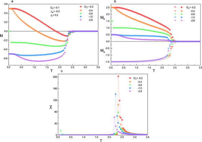
Figure 3. The influence of Db on the M, Ma, Mb, χ with fixed Da = −0.1, Jab = −0.2, and Jb = 0.2. |
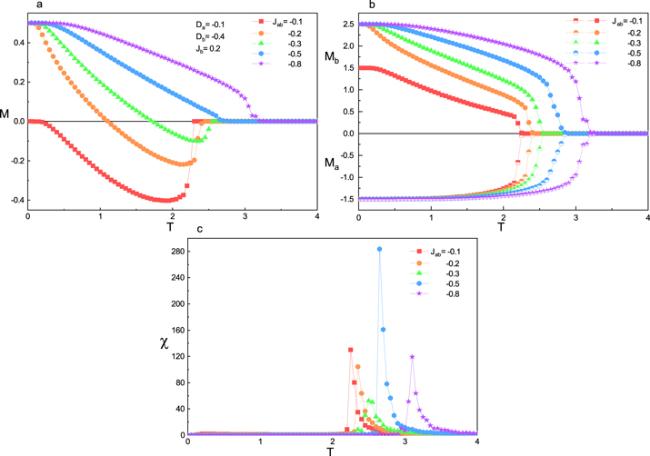
Figure 4. The influence of Jab on the M, Ma, Mb, χ with fixed Da = −0.1, Db = −0.4, and Jb = 0.2. |
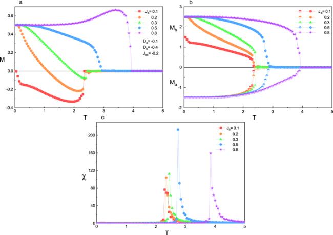
Figure 5. The influence of Jb on the M, Ma, Mb, χ with fixed Da = −0.1, Db = −0.4, and Jab = −0.2. |
Figures 5(a)–(c) present the influence of Jb on M, Ma, Mb, and χ with fixed Da = −0.1, Db = −0.4, and Jab = −0.2. In figure 5(a), the two saturation values (M = 0, 0.5) are also found for different values of Jb. And there are N-type curves for Jb = 0.2, 0.3, and P-type curves for Jb = 0.8 as predicted in $N\acute{e}{el}$ theory [37]. With Jb increasing, Tcomp is gradually moving to the high-temperature region, and the χ curves also shift right as shown in figure 5(c).
3.2. Phase diagram
To further examine the change of TC and Tcomp with various physical parameters, we plot the phase diagrams in different planes in figures 6(a)–(d). Every phase diagram is divided into paramagnetic (PF) and ferrimagnetic phases (FI) through the TC curve in each figure. In addition, we also find an interesting phenomenon that there is a critical value of every parameter (Da, Db, Jab, and Jb) that determines whether the graphene-like bilayer can display the compensation temperature. For example, these critical values of the parameters are Da = −1.4, Db = −0.12, Jab = −0.4, and Jb = 0.4, respectively. It can be observed from figures 6(a)–(b) that the value of TC becomes smaller with the crystal field increasing. However, the influence of Da and Db on Tcomp is the opposite. In figure 6(a), the value of Tcomp becomes bigger with $\left|{D}_{a}\right|$ increasing and when $\left|{D}_{a}\right|$ increases to 1.4, Tcomp disappears. But in figure 6(b), the stronger $\left|{D}_{b}\right|$, the smaller value of Tcomp, which reflects that the stronger $\left|{D}_{b}\right|$ promotes the appearance of compensation behavior. In figures 6(c) and 6(d), we can find that the stronger exchange couplings Jab and Jb can increase the value of TC, which is opposite to the effect of Da and Db on TC. And the weaker the exchange coupling, the more easily the compensation temperature appears. It has been also experimentally found that the magnetic anisotropy and the exchange coupling have a great influence on the phase transition of graphene-like layered structures. Namely, the stronger magnetic anisotropy and the weak interlayer exchange coupling are more conducive to the phase transition of the graphene-CrI3 system [42, 43]. This behavior can be compared with ours in figure 6.
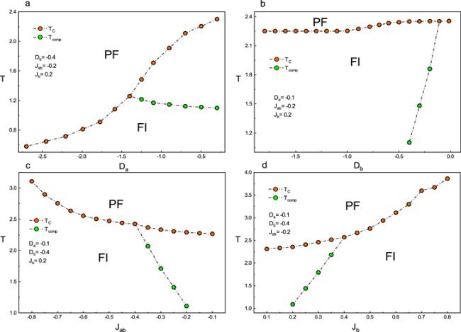
Figure 6. a. The phase diagram in the (T, Da) plane with Db = −0.4, Jab = −0.2, and Jb = 0.2. b. The phase diagram in the (T, Db) plane with Da = −0.1, Jab = −0.2, and Jb = 0.2. c. The phase diagram in the (T, Jab) plane with Da = −0.1, Db = −0.4, and Jb = 0.2. d. The phase diagram in the (T, Jb) plane with Da = −0.1, Db = −0.4, and Jab = −0.2. |
3.3. Specific heat, internal energy
Figures 7(a)–(b) show the influence of Da on the C and U with Db = −0.4, Jab = −0.2, and Jb = 0.2. In figure 7(a), with the increasing of $\left|{D}_{a}\right|$, the values of T corresponding to the peaks of the C curves become lower. In addition, we can clearly find in figure 7(b) that at fixed T, the stronger the $\left|{D}_{a}\right|$, the higher the U. This indicates that the system becomes more disordered with $\left|{D}_{a}\right|$ increasing.
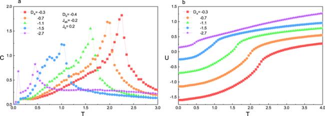
Figure 7. The influence of Da on C and U with fixed Db = −0.4, Jab = −0.2, and Jb = 0.2. |
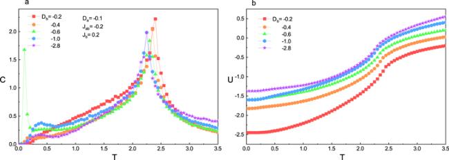
Figure 8. The influence of Db on C and U with fixed Da = −0.1, Jab = −0.2, and Jb = 0.2. |
The effect of Jab on the C and U with fixed Da = −0.1, Db = −0.4, and Jb = 0.2 is given in figures 9(a)–(b). Contrary to the rules of figures 7(a) and 8(a), with $\left|{J}_{{ab}}\right|$ increasing, the C curve moves to the high-temperature zone. It is interesting that there are two peaks in the C curve when Jab = −0.1. This is caused by the thermal disturbance of the system in the low-temperature zone. And we can find that the value of U becomes smaller under the greater value of $\left|{J}_{{ab}}\right|$, suggesting that the system becomes more stable for the stronger exchange coupling.
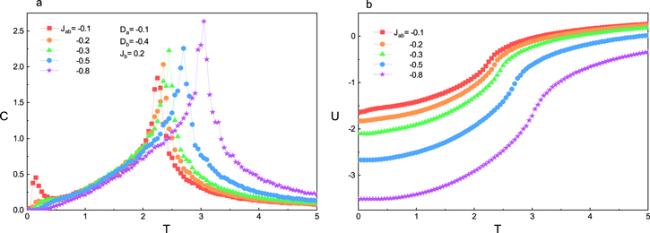
Figure 9. The influence of Jab on C and U with fixed Da = −0.1, Db = −0.4, and Jb = 0.2. |
We plot figures 10(a)–(b) to search the influence of Jb on the C and U with fixed Da = −0.1, Db = −0.4, and Jab = −0.2. One can see from figure 10(a) that the value of T corresponding to the peak of the C curve becomes higher with Jb increasing. In addition, in figure 10(b), the U is reduced at a certain temperature as Jb increases.
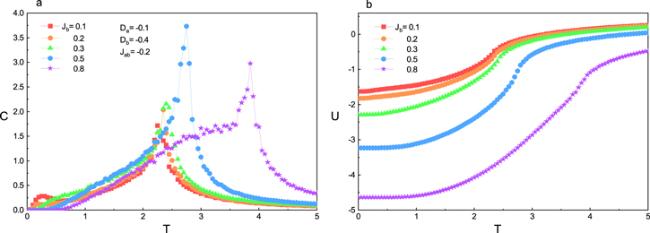
Figure 10. The influence of Jb on C and U with fixed Da = −0.1, Db = −0.4, and Jab = −0.2. |
3.4. Hysteresis loop
Figure 11 shows how Da affects the hysteresis loops of the whole system with Db = −1.0, Jab = −0.8, Jb = 1.0, and T = 0.5. There are triple loops when Da = −0.1 in figure 11(a), resulting from the competition among the external field, exchange coupling, and crystal field. For one thing, the spins of sublattices a and b tend to align along the direction of the strong external field. For another, the exchange coupling between two sublattices can prompt those spins to an antiparallel arrangement, and the strong crystal field can enrich more spin states. In addition, we can also find that when Da is changed from −0.1 to −0.7, the number of hysteresis loops is also changed from three to one, and the area of the hysteresis loop also decreases.
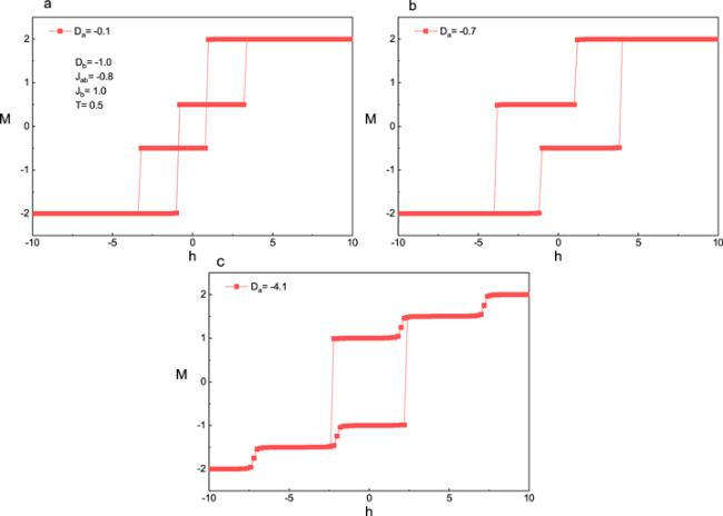
Figure 11. The influence of Da on the hysteresis loops of the system when Db = −1.0, Jab = −0.8, Jb = 1.0, and T = 0.5. |
Figure 12 shows the hysteresis loops caused by Db with Da = −0.5, Jab = −0.8, Jb = 1.0, and T = 0.5. It can be clearly observed that the number of the hysteresis loops is three when Db = −1.2. Similarly, we find the same rules in figure 12 as in 11, in which Db can also reduce the area of hysteresis loops.
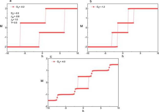
Figure 12. The influence of Db on the hysteresis loops of the system when Da = −0.5, Jab = −0.8, Jb = 1.0, and T = 0.5. |
The influence of Jab on the hysteresis loops is presented in figure 13 when Da = −0.5, Db = −1.0, Jab = −0.8, and T = 0.5. When Jab = −1.8, the triple hysteresis loops appear. Compared with the conclusions of figures 11 and 12, the effect of Jab is the opposite, in which increasing $\left|{J}_{{ab}}\right|$ can increase the area of the hysteresis loops.
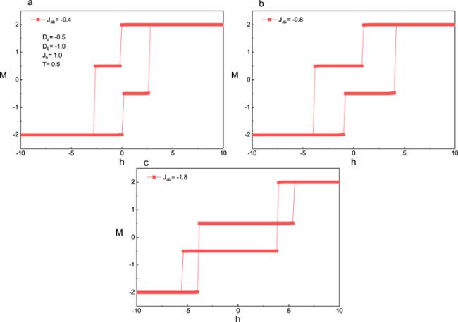
Figure 13. The influence of Jab on the hysteresis loops of the system when Da = −0.5, Db = −1.0, Jb = 1.0, and T = 0.5. |
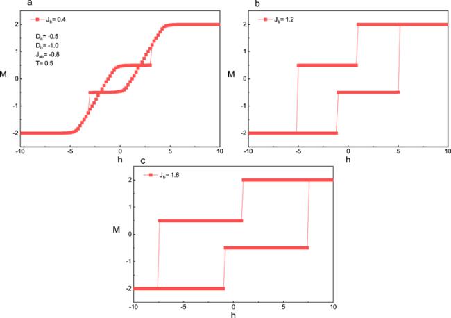
Figure 14. The influence of Jb on the hysteresis loops of the system when Da = −0.5, Db = −1.0, Jab = −0.8, and T = 0.5. |
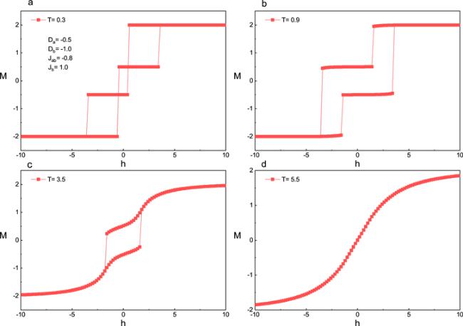
Finally, figure 15 presents the effect of T on the hysteresis loops when Da = −0.5, Db = −1.0, Jab = −0.8, and Jb = 1.0. From figures 15(a)–(d), at T = 0.3, the system shows the triple-loop hysteresis behavior. Further increasing T, the hysteresis loop turns into the single loop, with the area of the loop decreasing. When increasing T to 5.5, the hysteresis behavior vanishes. It indicates that the system becomes paramagnetic and the magnetization of the system is completely controlled by the external magnetic field and temperature. Similar hysteresis behaviors have been found both experimentally and theoretically. For instance, L. Fu et al have found that the coercivity and the remanence of bilayer graphene decrease with the temperature increasing. The area of hysteresis loops also becomes smaller with T increasing [44]. In addition, our results also agree well with those of the theoretical investigations of other low-dimensional structures [28, 45–50] and experimental research of graphene-CrI3 films [41], graphene nanoribbons [51], and graphene monolayers [52].
Figure 15. The influence of T on the hysteresis loops of the system when Da = −0.5, Db = −1.0, Jab = −0.8, and Jb = 1.0. |
4. Conclusion
By using the Monte Carlo method, we researched the compensation temperature and hysteresis behaviors of the ferrimagnetic graphene-like bilayer. The results show that the compensation behavior appears more easily by decreasing $\left|{J}_{{ab}}\right|,{J}_{b}$ and $\left|{D}_{a}\right|$, whereas the increase of $\left|{D}_{b}\right|$ can also prompt the appearance of the compensation behavior. In phase diagrams, we obtain four critical values of physical parameters that are related to the existence of compensation temperature. Finally, under the physical parameters, the triple-loop hysteresis behavior can be observed. The conclusions may offer a meaningful reference for the research of graphene-like layered films.