


1. Introduction
The study of constructing solutions to nonlinear evolution equations (NLEEs) has received much attention [1–9]. NLEEs can be used to model various nonlinear waves in the nature [10–18]. A considerable number of NLEEs can be solved exactly in many ways, such as the inverse scattering method [19], the Bäcklund transformation [20] and the Hirota bilinear method [21]. The inverse scattering method provides an efficient tool to solve initial value problems and needs strong assumptions about NLEEs [19]. With the Bäcklund transformation, the N-soliton solutions and infinite conservation laws can be derived by algebraic procedures [20]. The Hirota bilinear method is another approach for finding N-soliton solutions to some NLEEs [21–25]. Based on the bilinear forms to NLEEs, other exact solutions, such as lump solutions, periodic solutions and interaction solutions, can be deduced via the test function method [26–33].
The test function method was firstly applied to construct the lump solutions to the Kadomtsev–Petviashvili (KP) equation in 2015 [34]. It is proved that positive quadratic functions can yield lump solutions to NLEEs under the logarithmic transformation of a dependent variable. Then the sufficient and necessary conditions for the existence of positive quadratic functions solutions to Hirota bilinear equations were given in 2017 [35]. Multiple lump solutions, including two-, four-, and eight-lump solutions to a (3+1)-dimensional Boiti-Leon-Manna-Pempinelli equation can be generated from the polynomial functions [36]. The interaction solutions, such as lump-periodic solutions, one-lump-one-stripe solutions, one-lump-one-soliton solutions, and even one-lump-multi-stripe solutions, can be derived by choosing different test functions [37–42]. The one-lump-one-stripe solutions and one-lump-one-soliton solutions to the KP equation have been constructed by assuming that the test function is a combination of quadratic functions with one exponential function, or quadratic functions with one hyperbolic cosine function, respectively [43, 44]. New and more general one-lump-one-soliton solutions to the KP equation have been derived with an optional decoupling condition approach [45]. Moreover, based on two kinds of test function, the necessary and sufficient conditions have been presented for one-lump-multi-stripe solutions and one-lump-multi-soliton solutions to NLEEs [46]. The necessary and sufficient conditions have been employed to construct the two kinds of interaction solutions to the (2+1)-dimensional Ito equation, the (2+1)-dimensional Nizhnik-Novikov-Veselov system and a (2+1)-dimensional generalized Korteweg–de Vries equation [46]. It should be noted that the test function method can also be used to construct exact solutions to some NLEEs with variable coefficients [47].
The KP equation1 ) can be applied to many fields, such as plasmas, Bose–Einstein condensate and nonlinear optics [50]. The lump solutions, one-lump-one-stripe solutions and one-lump-one-soliton to equation (1 ) with σ = 1 have been derived based on the test function method [34, 43–45]. The long wave limit method was employed to obtain the M-lump solutions to equation (1 ) with σ = 1 [51]. Equation (1 ) enjoys the following bilinear form
$\begin{eqnarray}{\left({u}_{t}+6{{uu}}_{x}+{u}_{{xxx}}\right)}_{x}-\sigma {u}_{{yy}}=0,\sigma =\pm 1,\end{eqnarray}$
is an integrable equation, possessing N-soliton solutions, infinite conservation laws and the Lax pair [48, 49]. Equation ( $\begin{eqnarray}({D}_{x}{D}_{t}+{D}_{x}^{4}-\sigma {D}_{y}^{2})f\cdot f=0,\end{eqnarray}$
under the transformation $u=2{\left[\mathrm{ln}\,f(x,y,t)\right]}_{{xx}}$, where the D-operators [21] are defined as follows $\begin{eqnarray*}\begin{array}{l}{D}_{x}^{\alpha }{D}_{y}^{\beta }{D}_{t}^{\gamma }(f\cdot g)={\left(\displaystyle \frac{\partial }{\partial x}-\displaystyle \frac{\partial }{\partial x^{\prime} }\right)}^{\alpha }{\left(\displaystyle \frac{\partial }{\partial y}-\displaystyle \frac{\partial }{\partial y^{\prime} }\right)}^{\beta }\\ \quad \times {\left.{\left(\displaystyle \frac{\partial }{\partial t}-\displaystyle \frac{\partial }{\partial t^{\prime} }\right)}^{\gamma }f(x,y,t)g(x^{\prime} ,y^{\prime} ,t^{\prime} )\right|}_{x^{\prime} =x,y^{\prime} =y,t^{\prime} =t.}\end{array}\end{eqnarray*}$
The extended (2+1)-dimensional shallow water wave equation3 ) have been derived with the help of a general Riemann theta function and Bell polynomials [53]. Moreover, the lump solutions and lump-kink solutions to equation (3 ) have been constructed via the test function method [52]. Equation (3 ) enjoys the following bilinear form
$\begin{eqnarray}{u}_{{yt}}+3{u}_{{xxxy}}-3{u}_{{xx}}{u}_{y}-3{u}_{x}{u}_{{xy}}+\kappa {u}_{{xy}}=0,\end{eqnarray}$
can describe the evolution of nonlinear shallow water wave propagation [52]. The periodic wave solutions to equation ( $\begin{eqnarray}({D}_{y}{D}_{t}+{D}_{x}^{3}{D}_{y}+\kappa {D}_{x}{D}_{y})f\cdot f=0,\end{eqnarray}$
where κ is a constant, under the transformation$u=-2{\left[\mathrm{ln}\,f(x,y,t)\right]}_{x}$.In the case of σ = 1 and κ = − 1, the combination version of equations (2 ) and (4 ) reads
$\begin{eqnarray}({D}_{x}{D}_{t}+{D}_{x}^{4}-{D}_{y}^{2}+{D}_{y}{D}_{t}+{D}_{x}^{3}{D}_{y}-{D}_{x}{D}_{y})f\cdot f=0,\end{eqnarray}$
which is corresponding to the (2+1)-dimensional nonlinear model $\begin{eqnarray}\begin{array}{l}{\left({u}_{t}+6{{uu}}_{x}+{u}_{{xxx}}\right)}_{x}-{u}_{{yy}}+{u}_{{xxxy}}+3{u}_{{xx}}\\ \quad \times {\int }_{-\infty }^{x}{u}_{y}\,{\rm{d}}x+6{u}_{x}{u}_{y}+3{{uu}}_{{xy}}+{u}_{{yt}}-{u}_{{xy}}=0,\end{array}\end{eqnarray}$
under the transformation $u=2{\left[\mathrm{ln}\,f(x,y,t)\right]}_{{xx}}$.This paper is concerned with equation (6 ), which is a new (2+1)-dimensional nonlinear model. There exist various and complicated factors to affect the generation and propagation of nonlinear waves. The nonlinearity and dispersion are two of the important factors, which determine the nonlinear perturbation and decay of waves, respectively. With the development of the computation technology, it is worth dealing with more complex factors by extending initial models. The dispersion terms in equation (6 ) contain all the dispersion terms in equations (1 ) and (3 ), such as the second-order dispersions uxt, uyt and −uxy, and the fourth-order dispersions uxxxx and uxxxy. There exist new nonlinear terms in equation (6 ), which are different from those in equations (1 ) and (3 ), such as $3{u}_{{xx}}{\int }_{-\infty }^{x}{u}_{y}\,{\rm{d}}x$, 6uxuy and 3uuxy. Equation (6 ) describes more nonlinear and dispersion effect and has potential application in physics. We would like to investigate the evolution of solutions to equation (6 ) under the recombination of dispersion and nonlinear terms. Moreover, the bilinear form equation (5 ) can be rewritten as $({D}_{x}+{D}_{y})({D}_{t}+{D}_{x}^{3}-{D}_{y})f\cdot f\,=\,0$, which provides the possibility for the existence of one-lump-multi-stripe solutions and one-lump-multi-soliton solutions. Reference [46] has given the necessary and sufficient conditions for one-lump-multi-stripe solutions and one-lump-multi-soliton solutions to NLEEs. We will apply the theory and method in Ref. [46] to study the two kinds of solutions to equation (6 ), which could model nonlinear waves in mathematical physics and explain some properties of nonlinear mechanism.
In what follows, the dynamic behaviors of the lump solutions to equation (6 ) will be discussed in section 2 . Then the one-lump-multi-stripe solutions to equation (6 ) will be constructed by the test function combining quadratic functions and multiple exponential functions in section 3 . The one-lump-multi-soliton solutions will be deduced by the test function combining quadratic functions and multiple hyperbolic cosine functions in section 4 . Some concluding remarks will be given in section 5 .
2. Lump solutions to equation (6 )
We begin with the following test function [34]
$\begin{eqnarray}f={g}^{2}+{h}^{2}+{a}_{9},\end{eqnarray}$
with $\begin{eqnarray*}\begin{array}{rcl}g & = & {a}_{1}x+{a}_{2}y+{a}_{3}t+{a}_{4},\\ h & = & {a}_{5}x+{a}_{6}y+{a}_{7}t+{a}_{8},\end{array}\end{eqnarray*}$
where ai (1 ≤ i ≤ 9) are arbitrary constants. Two conditions a1a6 − a2a5 ≠ 0 and a9 > 0 need to be satisfied to guarantee the analyticity of lump solutions.Substituting equation (7 ) into equation (5 ) and making all the coefficients of each power of x, y, t to zero yield two sets of relations among ai (i = 1, 2,…,9)
Case 1
$\begin{eqnarray}\begin{array}{l}\left\{{a}_{2}=-\displaystyle \frac{{a}_{1}^{2}+{a}_{5}^{2}+{a}_{5}{a}_{6}}{{a}_{1}},\right.\\ \left.{a}_{3}=-\displaystyle \frac{{a}_{1}^{2}+{a}_{5}^{2}+{a}_{5}{a}_{6}}{{a}_{1}},\,{a}_{7}={a}_{6}\right\},\end{array}\end{eqnarray}$
Case 2
$\begin{eqnarray}\left\{{a}_{1}=-{a}_{3},\,{a}_{2}={a}_{3},\,{a}_{5}=0,\,{a}_{7}={a}_{6}\right\}.\end{eqnarray}$
Taking the Case 1 as an example, we obtain the lump solutions to equation (6 )
$\begin{eqnarray}u=\displaystyle \frac{4({a}_{1}^{2}+{a}_{5}^{2})}{f}-\displaystyle \frac{8{\left({a}_{1}g+{a}_{5}h\right)}^{2}}{{f}^{2}},\end{eqnarray}$
where $\begin{eqnarray*}\begin{array}{rcl}f & = & {\left({a}_{1}x-\displaystyle \frac{{a}_{1}^{2}+{a}_{5}^{2}+{a}_{5}{a}_{6}}{{a}_{1}}y-\displaystyle \frac{{a}_{1}^{2}+{a}_{5}^{2}+{a}_{5}{a}_{6}}{{a}_{1}}t+{a}_{4}\right)}^{2}\\ & & +{\left({a}_{5}x+{a}_{6}y+{a}_{6}t+{a}_{8}\right)}^{2}+{a}_{9},\\ g & = & {a}_{1}x-\displaystyle \frac{{a}_{1}^{2}+{a}_{5}^{2}+{a}_{5}{a}_{6}}{{a}_{1}}y-\displaystyle \frac{{a}_{1}^{2}+{a}_{5}^{2}+{a}_{5}{a}_{6}}{{a}_{1}}t+{a}_{4},\\ h & = & {a}_{5}x+{a}_{6}y+{a}_{6}t+{a}_{8}.\end{array}\end{eqnarray*}$
One maximum point and two minimum points of the lump wave locate at6 ) is shown in figure 1. The amplitude of the lump wave is constant, and it moves with the velocity (vx = 0, vy = − 1).
$\begin{eqnarray}\begin{array}{l}\left(x=-\displaystyle \frac{{a}_{1}^{2}{a}_{8}+{a}_{5}^{2}{a}_{8}+{a}_{1}{a}_{4}{a}_{6}+{a}_{5}{a}_{6}{a}_{8}}{({a}_{1}^{2}+{a}_{5}^{2})({a}_{5}+{a}_{6})},\right.\\ \left.y=-t-\displaystyle \frac{{a}_{1}({a}_{1}{a}_{8}-{a}_{4}{a}_{5})}{({a}_{1}^{2}+{a}_{5}^{2})({a}_{5}+{a}_{6})}\right),\end{array}\end{eqnarray}$
and $\begin{eqnarray}\begin{array}{l}\left(x=-\displaystyle \frac{\left({a}_{1}^{2}{a}_{8}+{a}_{5}^{2}{a}_{8}+{a}_{1}{a}_{4}{a}_{6}+{a}_{5}{a}_{6}{a}_{8}\right)}{({a}_{1}^{2}+{a}_{5}^{2})({a}_{5}+{a}_{6})}\right.\\ \quad \pm \displaystyle \frac{\sqrt{3{a}_{9}({a}_{1}^{2}+{a}_{5}^{2})}}{{a}_{1}^{2}+{a}_{5}^{2}},\\ \left.y=-t-\displaystyle \frac{{a}_{1}({a}_{1}{a}_{8}-{a}_{4}{a}_{5})}{({a}_{1}^{2}+{a}_{5}^{2})({a}_{5}+{a}_{6})}\right),\end{array}\end{eqnarray}$
respectively. These results indicate that the velocity of the lump wave is (vx = 0, vy = − 1), which is independent of the variables ai (1 ≤ i ≤ 9). By taking a selection of the variables, the evolution of lump solutions to equation (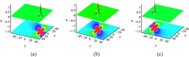
Figure 1. The evolution of lump solutions to equation ( |
3. One-lump-multi-stripe solutions to equation (6 )
By assuming that θi = ki1x + ki2y + ki3t + ki4 with θi ≠ θj (i ≠ j) and ${k}_{i1}{k}_{i3}+{k}_{i1}^{4}-{k}_{i2}^{2}+{k}_{i2}{k}_{i3}+{k}_{i1}^{3}{k}_{i2}-{k}_{i1}{k}_{i2}=0$, then the test function $f={g}^{2}+{h}^{2}+{a}_{9}+{\sum }_{i=1}^{N}{e}^{{\theta }_{i}}$ can generate the one-lump-multi-stripe solutions [46] to equation (6 ), if and only if
$\begin{eqnarray}\left\{\begin{array}{l}F({D}_{x},{D}_{y},{D}_{t})({g}^{2}+{h}^{2}+{a}_{9})\cdot ({g}^{2}+{h}^{2}+{a}_{9})=0,\\ F({D}_{x},{D}_{y},{D}_{t})({g}^{2}+{h}^{2}+{a}_{9})\cdot {e}^{{\theta }_{i}}=0,\,\,i=1,2,\cdots ,N,\\ F({k}_{i1}-{k}_{j1},{k}_{i2}-{k}_{j2},{k}_{i3}-{k}_{j3})=0,\,\,i\ne j,\,i,j=1,2,\cdots ,N,\end{array}\right.\end{eqnarray}$
where F(x, y, t) = xt + x4 − y2 + yt + x3y − xy. The proof can be referred to Ref. [46].Solving equation (13 ), we obtain two relations among ai (i = 1, 2,…,9) and kjm (j = 1, 2, ⋯ ,N, m = 1, 2, 3, 4)
Case 1
$\begin{eqnarray}\left\{\begin{array}{c}{a}_{2}=-\displaystyle \frac{{a}_{1}^{2}+{a}_{5}^{2}+{a}_{5}{a}_{6}}{{a}_{1}},\,{a}_{3}=-\displaystyle \frac{{a}_{1}^{2}+{a}_{5}^{2}+{a}_{5}{a}_{6}}{{a}_{1}},\,{a}_{7}={a}_{6},\\ {k}_{i2}=-{k}_{i1},\,{k}_{i3}=-{k}_{i1}-{k}_{i1}^{3},\,i=1,2,\cdots ,N\end{array}\right\},\end{eqnarray}$
Case 2
$\begin{eqnarray}\left\{\begin{array}{c}{a}_{1}=-{a}_{3},\,{a}_{2}={a}_{3},\,{a}_{5}=0,\,{a}_{7}={a}_{6},\,{k}_{i2}=-{k}_{i1},\,{k}_{i3}=-{k}_{i1}-{k}_{i1}^{3},\,i=1,2,\cdots ,N\end{array}\right\}.\end{eqnarray}$
Since the one-lump-multi-stripe solution in Case 2 has similar properties to that in Case 1, we take the Case 1 as an example, and the one-lump-multi-stripe solutions to equation (6 ) are
$\begin{eqnarray}\begin{array}{rcl}u & = & \displaystyle \frac{2\left(2{a}_{1}^{2}+2{a}_{5}^{2}+{\sum }_{i=1}^{N}{k}_{i1}^{2}{e}^{{\theta }_{i}}\right)}{f}\\ & & -\displaystyle \frac{2{\left(2{a}_{1}g+2{a}_{5}h+{\sum }_{i=1}^{N}{k}_{i1}{e}^{{\theta }_{i}}\right)}^{2}}{{f}^{2}},\end{array}\end{eqnarray}$
where $\begin{eqnarray*}\begin{array}{rcl}f & = & {\left({a}_{1}x-\displaystyle \frac{{a}_{1}^{2}+{a}_{5}^{2}+{a}_{5}{a}_{6}}{{a}_{1}}y-\displaystyle \frac{{a}_{1}^{2}+{a}_{5}^{2}+{a}_{5}{a}_{6}}{{a}_{1}}t+{a}_{4}\right)}^{2}\\ & & +{\left({a}_{5}x+{a}_{6}y+{a}_{6}t+{a}_{8}\right)}^{2}+{a}_{9}+\displaystyle \sum _{i=1}^{N}{e}^{{\theta }_{i}},\\ g & = & {a}_{1}x-\displaystyle \frac{{a}_{1}^{2}+{a}_{5}^{2}+{a}_{5}{a}_{6}}{{a}_{1}}y-\displaystyle \frac{{a}_{1}^{2}+{a}_{5}^{2}+{a}_{5}{a}_{6}}{{a}_{1}}t+{a}_{4},\\ h & = & {a}_{5}x+{a}_{6}y+{a}_{6}t+{a}_{8},\\ {\theta }_{i} & = & {k}_{i1}x-{k}_{i1}y-({k}_{i1}+{k}_{i1}^{3})t+{k}_{i4},\,i=1,2,\cdots ,N,\end{array}\end{eqnarray*}$
while a1a6 − a2a5 ≠ 0 and a9 > 0.The one-lump-one-stripe solutions to equation (6 ) are
$\begin{eqnarray}\begin{array}{rcl}u & = & \displaystyle \frac{2\left(2{a}_{1}^{2}+2{a}_{5}^{2}+{k}_{11}^{2}{e}^{{\theta }_{1}}\right)}{f}\\ & & -\displaystyle \frac{2{\left(2{a}_{1}g+2{a}_{5}h+{k}_{11}{e}^{{\theta }_{1}}\right)}^{2}}{{f}^{2}},\end{array}\end{eqnarray}$
where $\begin{eqnarray*}\begin{array}{rcl}f & = & {\left({a}_{1}x-\displaystyle \frac{{a}_{1}^{2}+{a}_{5}^{2}+{a}_{5}{a}_{6}}{{a}_{1}}y-\displaystyle \frac{{a}_{1}^{2}+{a}_{5}^{2}+{a}_{5}{a}_{6}}{{a}_{1}}t+{a}_{4}\right)}^{2}\\ & & +{\left({a}_{5}x+{a}_{6}y+{a}_{6}t+{a}_{8}\right)}^{2}+{a}_{9}+{e}^{{\theta }_{1}},\\ g & = & {a}_{1}x-\displaystyle \frac{{a}_{1}^{2}+{a}_{5}^{2}+{a}_{5}{a}_{6}}{{a}_{1}}y-\displaystyle \frac{{a}_{1}^{2}+{a}_{5}^{2}+{a}_{5}{a}_{6}}{{a}_{1}}t+{a}_{4},\\ h & = & {a}_{5}x+{a}_{6}y+{a}_{6}t+{a}_{8},\\ {\theta }_{1} & = & {k}_{11}x-{k}_{11}y-({k}_{11}+{k}_{11}^{3})t+{k}_{14},\end{array}\end{eqnarray*}$
while a1a6 − a2a5 ≠ 0 and a9 > 0.The one-lump-two-stripe solutions to equation (6 ) are
$\begin{eqnarray}\begin{array}{rcl}u & = & \displaystyle \frac{2\left(2{a}_{1}^{2}+2{a}_{5}^{2}+{k}_{11}^{2}{e}^{{\theta }_{1}}+{k}_{21}^{2}{e}^{{\theta }_{2}}\right)}{f}\\ & & -\displaystyle \frac{2{\left(2{a}_{1}g+2{a}_{5}h+{k}_{11}{e}^{{\theta }_{1}}+{k}_{21}{e}^{{\theta }_{2}}\right)}^{2}}{{f}^{2}},\end{array}\end{eqnarray}$
where $\begin{eqnarray*}\begin{array}{rcl}f & = & \left({a}_{1}x-\displaystyle \frac{{a}_{1}^{2}+{a}_{5}^{2}+{a}_{5}{a}_{6}}{{a}_{1}}y\right.\\ & & {\left.-\displaystyle \frac{{a}_{1}^{2}+{a}_{5}^{2}+{a}_{5}{a}_{6}}{{a}_{1}}t+{a}_{4}\right)}^{2}\\ & & +{\left({a}_{5}x+{a}_{6}y+{a}_{6}t+{a}_{8}\right)}^{2}+{a}_{9}+{e}^{{\theta }_{1}}+{e}^{{\theta }_{2}},\\ g & = & {a}_{1}x-\displaystyle \frac{{a}_{1}^{2}+{a}_{5}^{2}+{a}_{5}{a}_{6}}{{a}_{1}}y\\ & & -\displaystyle \frac{{a}_{1}^{2}+{a}_{5}^{2}+{a}_{5}{a}_{6}}{{a}_{1}}t+{a}_{4},\\ h & = & {a}_{5}x+{a}_{6}y+{a}_{6}t+{a}_{8},\\ {\theta }_{1} & = & {k}_{11}x-{k}_{11}y-({k}_{11}+{k}_{11}^{3})t+{k}_{14},\\ {\theta }_{2} & = & {k}_{21}x-{k}_{21}y-({k}_{21}+{k}_{21}^{3})t+{k}_{24},\end{array}\end{eqnarray*}$
while a1a6 − a2a5 ≠ 0 and a9 > 0.The one-lump-three-stripe solutions to equation (6 ) are
$\begin{eqnarray}\begin{array}{rcl}u & = & \displaystyle \frac{2\left(2{a}_{1}^{2}+2{a}_{5}^{2}+{k}_{11}^{2}{e}^{{\theta }_{1}}+{k}_{21}^{2}{e}^{{\theta }_{2}}+{k}_{31}^{2}{e}^{{\theta }_{3}}\right)}{f}\\ & & -\displaystyle \frac{2{\left(2{a}_{1}g+2{a}_{5}h+{k}_{11}{e}^{{\theta }_{1}}+{k}_{21}{e}^{{\theta }_{2}}+{k}_{31}{e}^{{\theta }_{3}}\right)}^{2}}{{f}^{2}},\end{array}\end{eqnarray}$
where $\begin{eqnarray*}\begin{array}{rcl}f & = & \left({a}_{1}x-\displaystyle \frac{{a}_{1}^{2}+{a}_{5}^{2}+{a}_{5}{a}_{6}}{{a}_{1}}y\right.\\ & & {\left.-\displaystyle \frac{{a}_{1}^{2}+{a}_{5}^{2}+{a}_{5}{a}_{6}}{{a}_{1}}t+{a}_{4}\right)}^{2}\\ & & +{\left({a}_{5}x+{a}_{6}y+{a}_{6}t+{a}_{8}\right)}^{2}+{a}_{9}\\ & & +{e}^{{\theta }_{1}}+{e}^{{\theta }_{2}}+{e}^{{\theta }_{3}},\\ g & = & {a}_{1}x-\displaystyle \frac{{a}_{1}^{2}+{a}_{5}^{2}+{a}_{5}{a}_{6}}{{a}_{1}}y\\ & & -\displaystyle \frac{{a}_{1}^{2}+{a}_{5}^{2}+{a}_{5}{a}_{6}}{{a}_{1}}t+{a}_{4},\\ h & = & {a}_{5}x+{a}_{6}y+{a}_{6}t+{a}_{8},\\ {\theta }_{1} & = & {k}_{11}x-{k}_{11}y-({k}_{11}+{k}_{11}^{3})t+{k}_{14},\\ {\theta }_{2} & = & {k}_{21}x-{k}_{21}y-({k}_{21}+{k}_{21}^{3})t+{k}_{24},\\ {\theta }_{3} & = & {k}_{31}x-{k}_{31}y-({k}_{31}+{k}_{31}^{3})t+{k}_{34},\end{array}\end{eqnarray*}$
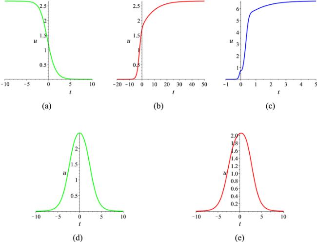
while a1a6 − a2a5 ≠ 0 and a9 > 0.Since ki1: ki2 = 1: − 1 (i = 1, 2, ⋯ ,N), all the stripe waves are parallel. The magnitudes of the velocities of the stripe waves and lump wave are $\tfrac{\sqrt{2}}{2}(1+{k}_{i1}^{2})\,(i=1,2,\cdots ,N)$ and $\tfrac{\sqrt{2}}{2}$, respectively. The direction of them is the vector (1, − 1). These facts indicate that the stripe waves move faster than the lump wave if ki1 ≠ 0 (i = 1, 2, ⋯ ,N). Figure 2 displays the evolution of one-lump-one-stripe solutions. There exist one lump wave and one stripe wave at t = −20. Since the stripe wave moves faster than the lump wave, the two waves collide with each other at t = − 2. Then the lump wave is gradually swallowed by the stripe wave. Figure 3 shows the fission process of one lump wave and two stripe waves. There exists one stripe wave at t = −20. The lump wave separates from the stripe wave at t = 3. one stripe wave splits into two stripe waves at t = 22. Figure 4 displays the nonelastic collisions among one lump wave and three stripe waves. The stripe wave s1 splits into two waves s2 and s3 at t = 2. Then the stripe wave s3 splits into two waves s4 and s5 at t = 3.5. The distance between the lump wave and the three stripe waves increases with time for the reason that the lump wave moves more slowly. Substituting equation (11 ) into equations (17 ), (18 ) and (19 ), we get the evolution of the amplitude of the lump waves shown in figure 7. The amplitude of the lump wave in figure 2 gradually decreases with time. Different from that, the amplitude of the lump wave in figures 3 and 4 gradually increases with time.
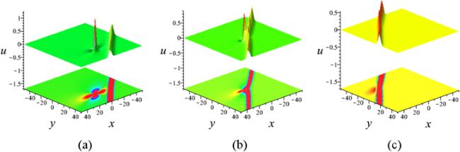
Figure 2. The evolution of one-lump-one-stripe solutions to equation ( |
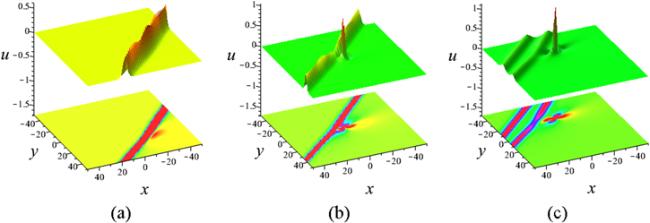
Figure 3. The evolution of one-lump-two-stripe solutions to equation ( |

Figure 4. The evolution of one-lump-three-stripe solutions to equation ( |
4. One-lump-multi-soliton solutions to equation (6 )
By assuming that θi = ki1x + ki2y + ki3t + ki4 with θi ≠ ± θj (i ≠ j) and ${k}_{i1}{k}_{i3}+{k}_{i1}^{4}-{k}_{i2}^{2}+{k}_{i2}{k}_{i3}+{k}_{i1}^{3}{k}_{i2}-{k}_{i1}{k}_{i2}=0$, g2 + h2 + a9 is a solution to equation (5 ), then the test function $f={g}^{2}+{h}^{2}+{a}_{9}+{\sum }_{i=1}^{N}\cosh {\theta }_{i}+c$, where c is a constant, can generate the one-lump-multi-soliton solutions [46] to equation (6 ), if and only if
$\begin{eqnarray}\left\{\begin{array}{l}F({D}_{x},{D}_{y},{D}_{t})({g}^{2}+{h}^{2}+{a}_{9})\cdot {e}^{{\theta }_{i}}=0,\,\,i=1,2,\cdots ,N,\\ F({k}_{i1}-{k}_{j1},{k}_{i2}-{k}_{j2},{k}_{i3}-{k}_{j3})=0,\,\,i\ne j,\,i,j=1,2,\cdots ,N,\\ F({k}_{i1}+{k}_{j1},{k}_{i2}+{k}_{j2},{k}_{i3}+{k}_{j3})=0,\,\,i\ne j,\,i,j=1,2,\cdots ,N,\\ F({D}_{x},{D}_{y},{D}_{t})({g}^{2}+{h}^{2}+{a}_{9})\cdot c+\displaystyle \sum _{i=1}^{N}\displaystyle \frac{1}{4}F(2{k}_{i1},2{k}_{i2},2{k}_{i3})=0.\end{array}\right.\end{eqnarray}$
The proof can be referred to Ref. [46].Solving equation (20 ), we obtain the same relations among ai (i = 1, 2,…,9) and kjm (j = 1, 2, ⋯ ,N, m = 1, 2, 3, 4) as equations (14 ) and (15 ). Since the one-lump-multi-soliton solution in Case 2 has similar properties to that in Case 1, we take the Case 1 as an example, and the one-lump-multi-soliton solutions to equation (6 ) are
$\begin{eqnarray}\begin{array}{rcl}u & = & \displaystyle \frac{2\left(2{a}_{1}^{2}+2{a}_{5}^{2}+\sum _{i=1}^{N}{k}_{i1}^{2}\cosh {\theta }_{i}\right)}{f}\\ & & -\displaystyle \frac{2{\left(2{a}_{1}g+2{a}_{5}h+\sum _{i=1}^{N}{k}_{i1}\sinh {\theta }_{i}\right)}^{2}}{{f}^{2}},\end{array}\end{eqnarray}$
where $\begin{eqnarray*}\begin{array}{rcl}f & = & \left({a}_{1}x-\displaystyle \frac{{a}_{1}^{2}+{a}_{5}^{2}+{a}_{5}{a}_{6}}{{a}_{1}}y\right.\\ & & {\left.-\displaystyle \frac{{a}_{1}^{2}+{a}_{5}^{2}+{a}_{5}{a}_{6}}{{a}_{1}}t+{a}_{4}\right)}^{2}\\ & & +{\left({a}_{5}x+{a}_{6}y+{a}_{6}t+{a}_{8}\right)}^{2}+{a}_{9}\\ & & +\displaystyle \sum _{i=1}^{N}\cosh {\theta }_{i}+c,\end{array}\end{eqnarray*}$
$\begin{eqnarray*}\begin{array}{rcl}g & = & {a}_{1}x-\displaystyle \frac{{a}_{1}^{2}+{a}_{5}^{2}+{a}_{5}{a}_{6}}{{a}_{1}}y-\displaystyle \frac{{a}_{1}^{2}+{a}_{5}^{2}+{a}_{5}{a}_{6}}{{a}_{1}}t+{a}_{4},\\ h & = & {a}_{5}x+{a}_{6}y+{a}_{6}t+{a}_{8},\\ {\theta }_{i} & = & {k}_{i1}x-{k}_{i1}y-({k}_{i1}+{k}_{i1}^{3})t+{k}_{i4},\,i=1,2,\cdots ,N,\end{array}\end{eqnarray*}$
while a1a6 − a2a5 ≠ 0, a9 > 0 and c ≥ 0.The one-lump-one-soliton solutions to equation (6 ) are
$\begin{eqnarray}\begin{array}{rcl}u & = & \displaystyle \frac{2\left(2{a}_{1}^{2}+2{a}_{5}^{2}+{k}_{11}^{2}\cosh {\theta }_{1}\right)}{f}\\ & & -\displaystyle \frac{2{\left(2{a}_{1}g+2{a}_{5}h+{k}_{11}\sinh {\theta }_{1}\right)}^{2}}{{f}^{2}},\end{array}\end{eqnarray}$
where $\begin{eqnarray*}\begin{array}{rcl}f & = & {\left({a}_{1}x-\displaystyle \frac{{a}_{1}^{2}+{a}_{5}^{2}+{a}_{5}{a}_{6}}{{a}_{1}}y-\displaystyle \frac{{a}_{1}^{2}+{a}_{5}^{2}+{a}_{5}{a}_{6}}{{a}_{1}}t+{a}_{4}\right)}^{2}\\ & & +{\left({a}_{5}x+{a}_{6}y+{a}_{6}t+{a}_{8}\right)}^{2}+{a}_{9}\\ & & +\cosh {\theta }_{1}+c,\end{array}\end{eqnarray*}$
$\begin{eqnarray*}\begin{array}{rcl}g & = & {a}_{1}x-\displaystyle \frac{{a}_{1}^{2}+{a}_{5}^{2}+{a}_{5}{a}_{6}}{{a}_{1}}y-\displaystyle \frac{{a}_{1}^{2}+{a}_{5}^{2}+{a}_{5}{a}_{6}}{{a}_{1}}t+{a}_{4},\\ h & = & {a}_{5}x+{a}_{6}y+{a}_{6}t+{a}_{8},\\ {\theta }_{1} & = & {k}_{11}x-{k}_{11}y-({k}_{11}+{k}_{11}^{3})t+{k}_{14},\end{array}\end{eqnarray*}$
while a1a6 − a2a5 ≠ 0, a9 > 0 and c ≥ 0.The one-lump-two-soliton solutions to equation (6 ) are
$\begin{eqnarray}\begin{array}{rcl}u & = & \displaystyle \frac{2\left(2{a}_{1}^{2}+2{a}_{5}^{2}+{k}_{11}^{2}\cosh {\theta }_{1}+{k}_{21}^{2}\cosh {\theta }_{2}\right)}{f}\\ & & -\displaystyle \frac{2{\left(2{a}_{1}g+2{a}_{5}h+{k}_{11}\sinh {\theta }_{1}+{k}_{21}\sinh {\theta }_{2}\right)}^{2}}{{f}^{2}},\end{array}\end{eqnarray}$
where $\begin{eqnarray*}\begin{array}{rcl}f & = & {\left({a}_{1}x-\displaystyle \frac{{a}_{1}^{2}+{a}_{5}^{2}+{a}_{5}{a}_{6}}{{a}_{1}}y-\displaystyle \frac{{a}_{1}^{2}+{a}_{5}^{2}+{a}_{5}{a}_{6}}{{a}_{1}}t+{a}_{4}\right)}^{2}\\ & & +{\left({a}_{5}x+{a}_{6}y+{a}_{6}t+{a}_{8}\right)}^{2}+{a}_{9}\\ & & +\cosh {\theta }_{1}+\cosh {\theta }_{2}+c,\end{array}\end{eqnarray*}$
$\begin{eqnarray*}\begin{array}{rcl}g & = & {a}_{1}x-\displaystyle \frac{{a}_{1}^{2}+{a}_{5}^{2}+{a}_{5}{a}_{6}}{{a}_{1}}y-\displaystyle \frac{{a}_{1}^{2}+{a}_{5}^{2}+{a}_{5}{a}_{6}}{{a}_{1}}t+{a}_{4},\\ h & = & {a}_{5}x+{a}_{6}y+{a}_{6}t+{a}_{8},\\ {\theta }_{1} & = & {k}_{11}x-{k}_{11}y-({k}_{11}+{k}_{11}^{3})t+{k}_{14},\\ {\theta }_{2} & = & {k}_{21}x-{k}_{21}y-({k}_{21}+{k}_{21}^{3})t+{k}_{24},\end{array}\end{eqnarray*}$
while a1a6 − a2a5 ≠ 0, a9 > 0 and c ≥ 0.Similar to the one-lump-multi-stripe solutions, the collision among one lump wave and soliton waves are nonelastic. The amplitude of the lump wave changes due to the collision with soliton waves. The one-lump-one-soliton solutions is shown in figure 5. The lump wave generates from the wave s1, then it is swallowed by the wave s2 because the lump wave moves more slowly than the wave s2. The evolution of one-lump-two-soliton solutions shown in figure 6 is more complicated. There exist multiple fusions and fissions of waves. Only two waves s1 and s2 appear at t = − 30. Then the wave s1 splits into s3 and s4. The wave s5 turns up because of the fusion of s2 and s4. The lump wave generates from s3, and is swallowed by s5. Finally, the fission (s3 → s6 + s7) and the fusion (s5 + s7 → s8) happen again. Substituting equation (11 ) into equations (22 ) and (23 ), we get the evolution of the amplitudes of the lump waves shown in figure 7. The amplitudes of the lump wave in figures 5 and 6 increase from 0 and then decrease to 0, which indicate that the collision among the lump wave and soliton waves are nonelastic.
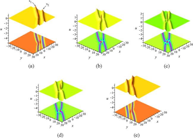
Figure 5. The evolution of the one-lump-one-soliton solutions to equation ( |
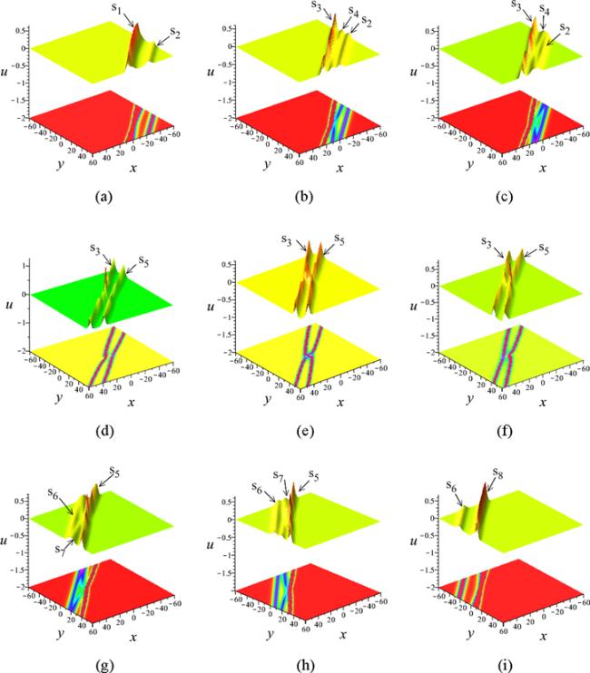
Figure 6. The evolution of the one-lump-two-soliton solutions to equation ( |
5. Conclusions
In this paper, we propose a combined form of bilinear KP equation and the bilinear extended (2+1)-dimensional shallow water wave equation, which is linked with a novel (2+1)-dimensional nonlinear model. Under the effect of a novel combination of nonlinearity and dispersion terms, two cases of lump solutions have been derived by searching for the quadratic function solutions to the bilinear form of equation (6 ). Taking the first case as an example, the velocity and amplitude of the lump wave are constant. There exist two types of one-lump-multi-stripe solutions. All the stripe waves are parallel and move faster than the lump wave as long as ki1 ≠ 0 (i = 1, 2, ⋯ ,N) in the test function. The lump wave and stripe waves move in the same direction, which is the vector (1, − 1). The lump wave can appear from the stripe waves or be swallowed by them. For the one-lump-multi-soliton solutions, the relations among ai (i = 1, 2,…,9) and kjm (j = 1, 2, ⋯ ,N, m = 1, 2, 3, 4) are the same as them in the one-lump-multi-stripe solutions. The collisions among one lump wave and soliton waves are nonelastic. The amplitude of the lump wave changes due to the collision with soliton waves. Based on the two test functions in this paper, there exist one-lump-multi-stripe solutions and one-lump-multi-soliton solutions to the extended (2+1)-dimensional shallow water wave equation. But there exist one-lump-one-stripe solutions and one-lump-one-soliton solutions to the KP equation. In this case, the extended (2+1)-dimensional shallow water wave equation has a greater impact in the analysis process of equation (6 ). Investigating the one-lump-multi-stripe solutions and one-lump-multi-soliton solutions is of importance to provide efficient expressions to model nonlinear waves and explain some interaction mechanism of nonlinear waves in physics. In the future, we will investigate the integrable properties of equation (6 ), such as Bäcklund transformations, Lax pairs and infinite conservation laws.
Acknowledgments
This work is supported by the Project of the Fundamental Research Funds for the Central Universities of China (2022JBMC034), the National Natural Science Foundation of China under Grant No. 12275017, and Beijing Laboratory of National Economic Security Early-warning Engineering, Beijing Jiaotong University.
Declaration of competing interest
The authors declare that they have no known competing financial interests or personal relationships that could have appeared to influence the work reported in this paper.
Data availability statement
All data, models, and code generated or used during the study appear in the submitted article.