


1. Introduction
The study of exotic hadrons with heavy quarks commenced with the discovery of the scalar charm-strange meson ${D}_{s0}^{* }(2317)$ decaying to ${D}_{s}^{+}{\pi }^{0}$ by the BaBar Collaboration [1] and the axial-vector charm-strange meson Ds1(2460) decaying to ${D}_{s}^{* +}{\pi }^{0}$ by the CLEO Collaboration [2]. In fact, in the BaBar data of the ${D}_{s}^{+}{\pi }^{0}\gamma $ invariant mass distribution with ${D}_{s}^{+}\gamma $ constrained in the ${D}_{s}^{* +}$ signal region, there is also a peak around 2.46 GeV [1], which could correspond to the Ds1(2460) state. No isospin partners for these states have been found, and their widths are extremely small, with upper bounds of 3.8 MeV and 3.5 MeV for the ${D}_{s0}^{* }(2317)$ and Ds1(2460), respectively [3]. Thus, these two mesons are isoscalar states. Since their masses are much lower than the quark model predictions of the lowest $c\bar{s}$ mesons with the corresponding JP quantum numbers [4], various models were proposed to understand them, including, for instance, modifying the $c\bar{s}$ quark model [5], interpreting the ${D}_{s0}^{* }(2317)$ and Ds1(2460) as D(*)K hadronic molecules, respectively [6–11], compact tetraquarks [12, 13], and chiral partners of the ground state Ds and ${D}_{s}^{* }$ mesons [14, 15]. Tremendous progress has been made towards understanding the ${D}_{s0}^{* }$ and Ds1, as well as their nonstrange partners, using lattice quantum chromodynamics or by analyzing the lattice data [16–30] (for a recent review, see [31]). Important information on the internal structure of these mesons can also be obtained from B(s) decays [32–35] and e+e− collisions [36].
Crucial observables to distinguish the hadronic molecular scenario from the others are the isospin breaking hadronic decay widths ${D}_{s0}^{* }(2317)\to {D}_{s}^{+}{\pi }^{0}$ and ${D}_{s1}(2460)\to {D}_{s}^{* +}{\pi }^{0}$, which are of the order of 100 keV for hadronic molecules [16, 25, 37] and much smaller in the other models [14, 38, 39]. The reason is that as D(*)K hadronic molecule, the ${D}_{s0}^{* }(2317)$ (Ds1(2460)) strongly couples to D(*)K and the isospin splittings of the charged and neutral D(*) and K mesons lead to significant isospin breaking effects since the respective poles are located rather close to the thresholds. Radiative decays of the ${D}_{s0}^{* }(2317)$ and Ds1(2460) have been computed in [37, 40–43] in the hadronic molecular model and in [14] in the chiral doublet model.
For the Ds1(2460), in addition to the isospin-breaking hadronic decay into the ${D}_{s}^{+}{\pi }^{0}$, also the decay into ${D}_{s}^{+}{\pi }^{+}{\pi }^{-}$ is allowed kinematically, respecting isospin symmetry, since the two pions can be in even partial waves and thus in an isoscalar state. The ratio of the partial width of this three-body decay relative to the two-body hadronic decay has been measured by the Belle Collaboration as [44]
$\begin{eqnarray}\displaystyle \frac{{\rm{\Gamma }}\left({D}_{s1}{\left(2460\right)}^{+}\to {D}_{s}^{+}{\pi }^{+}{\pi }^{-}\right)}{{\rm{\Gamma }}\left({D}_{s1}{\left(2460\right)}^{+}\to {D}_{s}^{* +}{\pi }^{0}\right)}=0.14\pm 0.04\pm 0.02,\end{eqnarray}$
while the value from the fit by the Particle Data Group (PDG) is 0.09 ± 0.02 [3]. Not much work has been done regarding the decay ${D}_{s1}{(2460)}^{+}\to {D}_{s}^{+}{\pi }^{+}{\pi }^{-}$. In [45], by treating the Ds1(2460) as a P-wave charm-strange meson, the width of the ${D}_{s1}{(2460)}^{+}\to {D}_{s}^{+}{\pi }^{+}{\pi }^{-}$ was predicted to be about 0.25 keV. In that work, the outgoing Ds is taken at rest such that the pion pair must be in a P-wave to conserve parity and angular momentum. Accordingly, in that work also the two-pion decay is isospin violating in contrast to our calculation, where the P-wave sits between the outgoing Ds and the isoscalar pion pair.The latest calculation of the width of ${D}_{s1}{(2460)}^{+}\to {D}_{s}^{* +}{\pi }^{0}$ within the D*K molecule scenario for Ds1(2460) is given in [43] where its value of (111 ± 15) keV is obtained from the complete isospin breaking contributions in the framework of unitarized chiral perturbation theory (UChPT) up to the next-to-leading order. In this work, we explicitly calculate the two-pion transitions and demonstrate that, assisted with the result of [43], the ratio in equation (1 ) is consistent with the D*K molecular picture for the Ds1(2460). We also show the internal structure of the Ds1(2460) leaves a characteristic imprint on the π+π− invariant mass distribution in the decay ${D}_{s1}{(2460)}^{+}\to {D}_{s}^{+}{\pi }^{+}{\pi }^{-}$.
Furthermore, predictions on the ${B}_{s1}\to {B}_{s}^{0}{\pi }^{+}{\pi }^{-}$ will be made, where the Bs1 is the bottom partner of the Ds1(2460).
2. Decay of the Ds1(2460)+ as a hadronic molecule into ${{\boldsymbol{D}}}_{{\boldsymbol{s}}}^{+}{\pi }^{+}{\pi }^{-}$
In this section, we calculate the decay width and π+π− invariant mass distribution of the ${D}_{s1}(2460)\to {D}_{s}^{+}{\pi }^{+}{\pi }^{-}$, taking into account the S-wave final-state interaction (FSI) between the two pions.
A crucial quantity distinguishing a hadronic molecular state from a compact state is the coupling of the state to the constituent hadrons, because the coupling squared is proportional to the probability of the physical state being composite [46–48]. Here we focus on the Ds1(2460). If the Ds1(2460) is a purely compact state with negligible D*K component, then its coupling to D*K would be negligibly small. In contrast, if the Ds1(2460) is a pure D*K bound state, then its coupling to D*K is maximal and the corresponding loops appear in all transitions at leading order, sometimes accompanied by short-ranged operators to absorb the pertinent divergences. The three-body decay into ${D}_{s}^{+}{\pi }^{+}{\pi }^{-}$ can proceed through the diagrams shown in figures 1 (a), (b) and (c). The loops are divergent and accordingly there is necessarily a counter term, shown as diagram (d), at the same order. In the molecular picture, the effect of this counter term can be estimated as (γ/β) = 25%, where β = 0.77 GeV is the mass of the lightest exchange particle allowed (in this case the ρ meson) and $\gamma =\sqrt{2\mu \epsilon }=0.19\,\mathrm{GeV}$ is the binding momentum, with μ for the reduced mass of the D*K system and ε = 45 MeV for the binding energy.7(7 Note that this estimate is built on the concept of resonance saturation which requires employing a natural cut-off in the calculation as we do it below [49].) If on the other hand, the Ds1(2460) were a compact state, the loops would be strongly suppressed and the transition amplitude would be dominated by diagram (d).
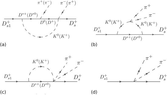
Figure 1. Diagrams for the decay ${D}_{s1}{(2460)}^{+}\to {D}_{s}^{+}{\pi }^{+}{\pi }^{-}$ with (a + b + c) and without (d) the D*K contribution. |
2.1. ${D}_{s1}{\left(2460\right)}^{+} \rightarrow {D}_{s}^{+}{\pi }^{+}{\pi }^{-}$ through the D*K component
Let us consider first the decay of the ${D}_{s1}{(2460)}^{+}\to {D}_{s}^{+}{\pi }^{+}{\pi }^{-}$ with the molecular assumption occurring through the one-loop triangle diagrams (a), (b) and (c) in figure 1. For the decay ${D}_{s1}(2460)\to {D}_{s}^{+}{\pi }^{+}{\pi }^{-}$ to keep isospin symmetry, the π+π− system in the final state must be an isospin scalar. Therefore, the quantum numbers of the π+π− system must be JPC = even++. Then the lowest partial wave between the π+π− system and ${D}_{s}^{+}$ is a P-wave.
To calculate the amplitudes for diagrams (a), (b) and (c) in figure 1, we employ the following effective Lagrangians for the Ds1D*K [42] and the other vertices [50, 51]
$\begin{eqnarray}{{ \mathcal L }}_{{{PD}}^{* \dagger }{D}_{s1}}=\displaystyle \frac{f}{\sqrt{2}}{D}_{s1}^{\mu }\left({D}_{\mu }^{* +\dagger }{K}^{0\dagger }+{D}_{\mu }^{* 0\dagger }{K}^{+\dagger }\right)+{\rm{h}}.{\rm{c}}.,\end{eqnarray}$
$\begin{eqnarray}\begin{array}{l}{{ \mathcal L }}_{\chi }=\displaystyle \frac{{F}_{\pi }^{2}}{4}\mathrm{Tr}\left[{\partial }_{\mu }U{\partial }^{\mu }{U}^{\dagger }\right]-\left\langle {H}_{a}({\rm{i}}v\cdot {{ \mathcal D }}_{{ab}}){\bar{H}}_{b}\right\rangle \\ \qquad +\,g\left\langle {H}_{a}\gamma \cdot {{ \mathcal A }}_{{ab}}{\gamma }_{5}{\bar{H}}_{b}\right\rangle ,\end{array}\end{eqnarray}$
where $U={u}^{2}=\exp (\sqrt{2}{\rm{i}}{\rm{\Phi }}/{F}_{\pi })$ is a nonlinear function of the field Φ for the light pseudoscalar Goldstone bosons with $\begin{eqnarray}{\rm{\Phi }}=\left(\begin{array}{ccc}\displaystyle \frac{{\pi }^{0}}{\sqrt{2}}+\displaystyle \frac{\eta }{\sqrt{6}} & {\pi }^{+} & {K}^{+}\\ {\pi }^{-} & -\displaystyle \frac{{\pi }^{0}}{\sqrt{2}}+\displaystyle \frac{\eta }{\sqrt{6}} & {K}^{0}\\ {K}^{-} & {\bar{K}}^{0} & -\displaystyle \frac{2\eta }{\sqrt{6}}\end{array}\right),\end{eqnarray}$
with Fπ the pion decay constant in the chiral limit. ${H}_{a}=1/2(1+v\cdot \gamma )[{P}_{a,\mu }^{* }{\gamma }^{\mu }-{P}_{a}{\gamma }_{5}]$, with a the light flavor index, is a superfield for the ground state pseudoscalar and vector heavy mesons, which are in the same heavy quark spin multiplet, where ${P}_{\mu }^{* }$ and P annihilate the vector and pseudoscalar heavy mesons, respectively. ${{ \mathcal D }}_{{ab}}^{\mu }={\delta }_{{ab}}{\partial }^{\mu }-{{ \mathcal V }}_{{ab}}^{\mu }$ is the chirally covariant derivative with ${{ \mathcal V }}_{\mu }=({u}^{\dagger }{\partial }_{\mu }u+u{\partial }_{\mu }{u}^{\dagger })/2$ the light meson vector current and ${{ \mathcal A }}_{\mu }\,={\rm{i}}({u}^{\dagger }{\partial }_{\mu }u-u{\partial }_{\mu }{u}^{\dagger })/2$ the corresponding axial current. Tr[·] and $\left\langle \cdot \right\rangle $ take traces in the flavor and spinor spaces, respectively.Since the Ds1(2460) mass is smaller than the D*K threshold by just about 45 MeV, the binding momentum of the Ds1(2460) as a D*K bound state is about 0.19 GeV, much smaller than both the kaon and D* masses. Thus, we may use a constant coupling for the Ds1D*K coupling in equation (2 ), following [42]. The coupling f squared can be computed from the residue of the unitarized D*K → D*K scattering amplitude in UChPT, and it is related to the ${D}_{s0}^{* }(2317){DK}$ coupling by means of heavy quark spin symmetry as done in [43]. We take $f={10.1}_{-0.9}^{+0.8}$ GeV from [43], which is the result in UChPT using the low-energy constants (LECs) determined in [16]. The axial coupling constant g is determined to be 0.565 ± 0.006 by reproducing the measured partial width of D*+ → D0π+, that is, (83.4 ± 1.8) keV for the total width of D*+ with the branching fraction 0.677 ± 0.005 [3]. For the pion decay constant, we use the physical value Fπ = 92 MeV.
The amplitude for the triangle diagrams in figure 1 is given by
$\begin{eqnarray}\begin{array}{l}{{ \mathcal M }}_{({\rm{a}})+({\rm{b}})+({\rm{c}})}={{ \mathcal M }}_{({\rm{a}})}+{{ \mathcal M }}_{({\rm{b}})}+{{ \mathcal M }}_{({\rm{c}})}+{{ \mathcal M }}_{({\rm{a}})}{| }_{{p}_{{\pi }^{+}}\leftrightarrow {p}_{{\pi }^{-}}}\\ \,+\,{{ \mathcal M }}_{({\rm{b}})}{| }_{{p}_{{\pi }^{+}}\leftrightarrow {p}_{{\pi }^{-}}}+{{ \mathcal M }}_{({\rm{c}})}{| }_{{p}_{{\pi }^{+}}\leftrightarrow {p}_{{\pi }^{-}}},\end{array}\end{eqnarray}$
where ${{ \mathcal M }}_{({\rm{a}})}$, ${{ \mathcal M }}_{({\rm{b}})}$ and ${{ \mathcal M }}_{({\rm{c}})}$ read $\begin{eqnarray}\begin{array}{l}{{ \mathcal M }}_{({\rm{a}})}=\displaystyle \frac{-{{fgM}}_{D}\sqrt{{M}_{{D}_{s}}{M}_{{D}^{* }}}}{2{F}_{\pi }^{3}}\int \displaystyle \frac{{{\rm{d}}}^{4}k}{{\left(2\pi \right)}^{4}}\\ \,\times \,\displaystyle \frac{{\rm{i}}v\cdot (k-{p}_{{D}_{s1}}-{p}_{{\pi }^{-}}){\epsilon }_{{D}_{s1}}^{(\lambda )}\cdot {p}_{{\pi }^{+}}}{({k}^{2}-{M}_{{D}^{* }}^{2})[{\left({p}_{{D}_{s1}}-k\right)}^{2}-{M}_{K}^{2}][{\left(k-{p}_{{\pi }^{+}}\right)}^{2}-{M}_{D}^{2}]},\end{array}\end{eqnarray}$
$\begin{eqnarray}\begin{array}{l}{{ \mathcal M }}_{({\rm{b}})}=\frac{{{fgM}}_{D}\sqrt{{M}_{{D}_{s}}{M}_{D}^{* }}}{12{F}_{\pi }^{3}}\int \frac{{{\rm{d}}}^{4}k}{{\left(2\pi \right)}^{4}}\\ \,\times \,\frac{-2{\rm{i}}{\epsilon }_{{D}_{s1}}^{(\lambda )}\cdot ({p}_{{D}_{s1}}-{p}_{{\pi }^{+}}-{p}_{{\pi }^{-}}-k)}{({k}^{2}-{M}_{{D}^{* }}^{2})[{\left({p}_{{D}_{s1}}-k\right)}^{2}-{M}_{K}^{2}][{\left({p}_{{D}_{s1}}-{p}_{{\pi }^{+}}-{p}_{{\pi }^{-}}-k\right)}^{2}-{M}_{K}^{2}]}\\ \,\times \,\left({M}_{{D}_{s1}}^{2}-{M}_{\pi }^{2}+{p}_{{D}_{s1}}\cdot (2{p}_{{\pi }^{-}}-4{p}_{{\pi }^{+}}-2k)\right.\\ \,\left.+\,{k}^{2}-2{p}_{{\pi }^{+}}\cdot {p}_{{\pi }^{-}}+k\cdot (4{p}_{{\pi }^{+}}-2{p}_{{\pi }^{-}}\right),\end{array}\end{eqnarray}$
$\begin{eqnarray}\begin{array}{l}{{ \mathcal M }}_{({\rm{c}})}=\displaystyle \frac{-{\rm{i}}{fg}\sqrt{{M}_{{D}_{s}}{M}_{{D}^{* }}}}{12{F}_{\pi }^{3}}\\ \,\times \int \displaystyle \frac{{{\rm{d}}}^{4}k}{{\left(2\pi \right)}^{4}}\displaystyle \frac{{\epsilon }_{{D}_{s1}}^{(\lambda )}\cdot ({p}_{{\pi }^{+}}-k-2{p}_{{\pi }^{-}})}{({k}^{2}-{M}_{K}^{2})[{\left({p}_{{D}_{s1}}^{}-k\right)}^{2}-{M}_{{D}^{* }}^{2}]}\,.\end{array}\end{eqnarray}$
Here, ${\epsilon }_{{D}_{s1}}^{(\lambda )}$ is the polarization vector of the Ds1, with λ denoting the polarization components, ${p}_{{D}_{s1}}$ is the four-momentum of the Ds1 meson, and ${p}_{{\pi }^{\pm }}$ is the four-momentum of the π± emitted from the Ds1 decay.In the UChPT calculation for the isospin-breaking hadronic decays and radiative decays of the Ds1(2460) and ${D}_{s0}^{* }(2317)$, a three-momentum cut-off ${q}_{\max }={745}_{-37}^{+35}\,\mathrm{MeV}$ is introduced [43]. Here, we use the same cut-off range for the loop integrals to ensure the treatment to be consistent with the calculation of the decay ${D}_{s1}{\left(2460\right)}^{+}\to {D}_{s}^{* +}{\pi }^{0}$ in [43].
2.2. Partial wave projection and the ππ FSI
Since the two pions can be in the isoscalar S-wave and the phase space allows the π+π− invariant mass to be up to 0.49 GeV, the ππ final state interaction (FSI) needs to be considered in the calculation of both the ${D}_{s1}(2460)\to {D}_{s}^{+}{\pi }^{+}{\pi }^{-}$ partial width and the corresponding π+π− invariant mass distribution. In particular, the f0(500) resonance, also known as the σ meson, contributes through the S-wave ππ FSI.
To that end, we briefly introduce the partial wave projection that is used to include the S-wave ππ FSI effect. We work in the rest frame of ${D}_{s1}{\left(2460\right)}^{+}$ and choose the positive z-axis to be along the moving direction of ${D}_{s}^{+}$. The decay amplitude ${ \mathcal M }$ of ${D}_{s1}{\left(2460\right)}^{+}\to {D}_{s}^{+}{\pi }^{+}{\pi }^{-}$ in equation (5 ) is a function of the polarization vector ${\epsilon }_{{D}_{s1}}^{(\lambda )}$ of Ds1 and two kinematic variables ${m}_{{\pi }^{+}{\pi }^{-}}$ and θ, i.e. ${ \mathcal M }={ \mathcal M }({m}_{{\pi }^{+}{\pi }^{-}},\theta ,{\epsilon }_{{D}_{s1}}^{(\lambda )})$, where ${m}_{{\pi }^{+}{\pi }^{-}}$ is the π+π− invariant mass and θ denotes the angle between the π+ moving direction in the center-of-mass (c.m.) frame of π+π− and the moving direction of the π+π− system in the Ds1 rest frame. Then the partial wave projection is carried out by means of the formula (see, e.g. [52])
$\begin{eqnarray}\begin{array}{l}{{ \mathcal M }}^{l}({m}_{{\pi }^{+}{\pi }^{-}})=\displaystyle \frac{2\pi {{\rm{Y}}}_{\bar{l}}^{0}(\hat{{\bf{z}}})}{2J+1}\displaystyle \sum _{\lambda ,m}\int \mathrm{dcos}\theta \,{{\rm{Y}}}_{l}^{m}{\left(\theta \right)}^{* }(m0m| {lSJ})\\ \,\times \,(0\lambda m| \bar{l}\bar{S}J){ \mathcal M }({m}_{{\pi }^{+}{\pi }^{-}},\theta ,{\epsilon }_{{D}_{s1}}^{(\lambda )}),\end{array}\end{eqnarray}$
where (mSzJz∣lSJ) are the Clebsch–Gordan coefficients for the coupling of orbital angular momentum l and spin S to the total angular momentum J, with m, Sz and Jz the corresponding third components, and ${{\rm{Y}}}_{l}^{m}(\theta )$ is the spherical harmonic function. Here, we use l, S and $\bar{l},\bar{S}$ to denote the quantum numbers of the π+π− and Ds1(2460)Ds systems, respectively. Thus, for the S-wave ππ, we have $\{J=0,l=S=0,\bar{l}=\bar{S}=1\};$ for the D-wave ππ, we have $\{J=l=2,S=0,\bar{l}=\bar{S}=1\}$ and $\{J=l=2,S=0,\bar{l}=3,\bar{S}=1\}$. Since the lightest tensor meson f2(1270) is far away from the region of interest, only the S-wave ππ FSI effect is taken into account.The ππ FSI for the decay ${D}_{s1}{\left(2460\right)}^{+}\to {D}_{s}^{+}{\pi }^{+}{\pi }^{-}$, as shown in figure 2, is taken into account using a dispersion relation approach with inhomogeneity inducing the left-hand cut contribution. A similar approach has been used in studying other hadronic processes, see e.g. [53–60]. Here, the inhomogeneity comes from the loop diagrams shown in figures 1 (a), (b) and (c). The decay amplitude ${{ \mathcal M }}_{{\pi }^{+}{\pi }^{-}}$ for the process ${D}_{s1}{\left(2460\right)}^{+}\to {D}_{s}^{+}{\pi }^{+}{\pi }^{-}$ with the S-wave ππ rescattering (here only the π0π0 and π+π− channels are relevant due to the phase space limitation, and the D-wave rescattering is negligible because the f2(1270) mass is much higher than the energy region of interest) included satisfies the unitarity relation10 ) and equation (12 ), one can obtain5 ).
$\begin{eqnarray}\begin{array}{l}\displaystyle \frac{1}{2{\rm{i}}}\mathrm{disc}\,{{ \mathcal M }}_{{\pi }^{+}{\pi }^{-}}^{00}=\displaystyle \frac{2}{3}{\left({t}_{0}^{0}\right)}^{* }{\sigma }_{\pi }{{ \mathcal M }}_{{\pi }^{+}{\pi }^{-}}^{00}\\ \quad +\displaystyle \frac{1}{3}{\left({t}_{0}^{0}\right)}^{* }{\sigma }_{\pi }{{ \mathcal M }}_{{\pi }^{0}{\pi }^{0}}^{00}={\left({t}_{0}^{0}\right)}^{* }{\sigma }_{\pi }{{ \mathcal M }}_{{\pi }^{+}{\pi }^{-}}^{00},\end{array}\end{eqnarray}$
where $\mathrm{disc}\,{{ \mathcal M }}_{{\pi }^{+}{\pi }^{-}}^{00}$ is the discontinuity of the ${D}_{s1}{\left(2460\right)}^{+}\to {D}_{s}^{+}{\pi }^{+}{\pi }^{-}$ amplitude in the isoscalar S partial wave along the ππ right-hand cut, starting from the ππ threshold to infinity along the positive real axis, and ${{ \mathcal M }}_{{\pi }^{0}{\pi }^{0}}^{00}$ is the decay amplitude of ${D}_{s1}{\left(2460\right)}^{+}\to {D}_{s}^{+}{\pi }^{0}{\pi }^{0}$ in the isoscalar S partial wave. For the second identity, ${{ \mathcal M }}_{{\pi }^{0}{\pi }^{0}}^{00}={{ \mathcal M }}_{{\pi }^{+}{\pi }^{-}}^{00}$ in the isospin limit is applied. Furthermore, ${\sigma }_{\pi }=\sqrt{1-4{M}_{\pi }^{2}/s}$ is the phase space factor of the two-pion channel with $\sqrt{s}={m}_{\pi \pi }$ the c.m. energy of the ππ system, ${t}_{0}^{0}$ represents the elastic isoscalar S-wave ππ scattering amplitude, and $\begin{eqnarray}{\left({t}_{0}^{0}\right)}^{* }{\sigma }_{\pi }={e}^{-{\rm{i}}{\delta }_{0}^{0}}\sin {\delta }_{0}^{0},\end{eqnarray}$
with ${\delta }_{0}^{0}$ the isoscalar S-wave ππ scattering phase shift. The Omnès function Ω(s) is introduced as the solution of the unitarity relation $\begin{eqnarray}\displaystyle \frac{1}{2{\rm{i}}}\mathrm{disc}\,{\rm{\Omega }}={\left({t}_{0}^{0}\right)}^{* }{\sigma }_{\pi }{\rm{\Omega }},\end{eqnarray}$
which can be solved by [61] $\begin{eqnarray}{\rm{\Omega }}(s)=\exp \left(\displaystyle \frac{s}{\pi }{\int }_{4{M}_{\pi }^{2}}^{\infty }\displaystyle \frac{{\rm{d}}{s}^{{\prime} }}{{s}^{{\prime} }}\displaystyle \frac{{\delta }_{0}^{0}({s}^{{\prime} })}{{s}^{{\prime} }-s-{\rm{i}}\epsilon }\right).\end{eqnarray}$
Starting from equation ( $\begin{eqnarray}\displaystyle \frac{1}{2{\rm{i}}}\mathrm{disc}\,\displaystyle \frac{{{ \mathcal M }}^{00}-{{ \mathcal M }}_{L}^{00}}{{\rm{\Omega }}}=\displaystyle \frac{1}{{\rm{\Omega }}}{\left({t}_{0}^{0}\right)}^{* }{\sigma }_{\pi }{{ \mathcal M }}_{L}^{00}=\displaystyle \frac{1}{| {\rm{\Omega }}| }\sin {\delta }_{0}^{0}{{ \mathcal M }}_{L}^{00},\end{eqnarray}$
where ${{ \mathcal M }}_{L}^{00}$ is the part of ${{ \mathcal M }}_{{\pi }^{+}{\pi }^{-}}^{00}$ containing only the inhomogeneity that is modeled by diagrams (a) + (b) + (c) in figure 1 in the present work, i.e. the S-wave projection of ${{ \mathcal M }}_{({\rm{a}})+({\rm{b}})+({\rm{c}})}$ in equation (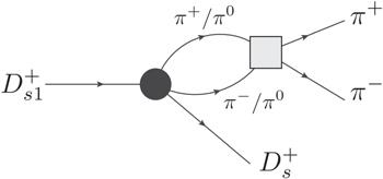
Figure 2. Diagram for the decay ${D}_{s1}{(2460)}^{+}\to {D}_{s}^{+}{\pi }^{+}{\pi }^{-}$ with the ππ FSI considered. The black circle denotes the amplitude of ${D}_{s1}{(2460)}^{+}\to {D}_{s}^{+}{\pi }^{+}{\pi }^{-}$ for the diagrams in figure 1 and similar loop diagram contributions to ${D}_{s1}{(2460)}^{+}\to {D}_{s}^{+}{\pi }^{0}{\pi }^{0}$. The square represents the pion–pion rescattering. |
Then one can write a once-subtracted dispersion relation for the decay amplitude of ${D}_{s1}{\left(2460\right)}^{+}\to {D}_{s}^{+}{\pi }^{+}{\pi }^{-}$ with the S-wave ππ FSI effect included15 ) can be interpreted diagrammatically. ${{ \mathcal M }}_{L}^{00}$ is the amplitude of diagrams (a), (b) and (c) in figure 1 projected to the ππ S-wave, as mentioned above. The second term in the square bracket (together with the Ω(s) factor outside) corresponds to the triangle diagrams connected to the ππ FSI. The subtraction term a Ω(s) corresponds to a Ds1Dsππ contact term connected to the ππ FSI, which can be expressed as
$\begin{eqnarray}\begin{array}{l}{{ \mathcal M }}^{00}(s)={{ \mathcal M }}_{L}^{00}+{\rm{\Omega }}(s)\left[a+\displaystyle \frac{s}{\pi }{\int }_{4{M}_{\pi }^{2}}^{{s}_{\max }}\,\displaystyle \frac{{\rm{d}}s^{\prime} }{s^{\prime} }\,\right.\\ \,\,\left.\times \,\displaystyle \frac{{{ \mathcal M }}_{L}^{00}\sin {\delta }_{0}^{0}(s^{\prime} )}{| {\rm{\Omega }}(s^{\prime} )| \,(s^{\prime} -s-{\rm{i}}\epsilon )}\right],\end{array}\end{eqnarray}$
where a is a subtraction constant. A single subtraction is sufficient to ensure the convergence as can be checked by varying the cut-off ${s}_{\max }$. Each term on the right-hand side of equation ( $\begin{eqnarray}{{ \mathcal M }}_{\mathrm{comp}.}^{00}(s)={g}_{c}\,{\epsilon }_{{D}_{s1}}\cdot {p}_{{D}_{s}}{\rm{\Omega }}(s),\end{eqnarray}$
where gc is a Ds1 → Dsπ+π− contact term coupling constant.As for the ππ scattering phase shift, we employ the following parameterization [62]
$\begin{eqnarray}{\delta }_{0}^{0}(s)=\left\{\begin{array}{ll}0, & 0\leqslant \sqrt{s}\leqslant 2{M}_{\pi },\\ {f}_{1}(s), & 2{M}_{\pi }\lt \sqrt{s}\leqslant \sqrt{{s}_{m}},\end{array}\right.\end{eqnarray}$
where $\begin{eqnarray}\begin{array}{l}{f}_{1}(s)=\mathrm{arccot}\left\{\displaystyle \frac{s}{\lambda {\left(s,{M}_{\pi }^{2},{M}_{\pi }^{2}\right)}^{1/2}}\displaystyle \frac{{M}_{\pi }^{2}}{s-{z}_{0}^{2}/2}\right.\\ \quad \left.\times \left[\displaystyle \frac{{z}_{0}^{2}}{{M}_{\pi }\sqrt{s}}+{B}_{0}+{B}_{1}w(s)+{B}_{2}{w}^{2}(s)+{B}_{3}{w}^{3}(s)\right]\right\}.\end{array}\end{eqnarray}$
The parameters of this expression $\begin{eqnarray*}\begin{array}{l}{z}_{0}={M}_{\pi },\quad {B}_{0}=7.14,\quad {B}_{1}=-25.3,\\ \quad {B}_{2}=-33.2,\quad {B}_{3}=-26.2,\end{array}\end{eqnarray*}$
were adjusted to the ππ scattering phase shifts extracted from a Roy-type analysis of the two-pion system, with $\begin{eqnarray}w(s)=\displaystyle \frac{\sqrt{s}-\sqrt{4{M}_{K}^{2}-s}}{\sqrt{s}+\sqrt{4{M}_{K}^{2}-s}}\end{eqnarray}$
and λ(x, y, z) = x2 + y2 + z2 − 2(xy + yz + zx) is the Källén function. Since here the phase space restricts the physical region of $\sqrt{s}$ to be less than 0.5 GeV, we only consider contributions from the ππ channel to the rescattering. Accordingly, the phase shift ${\delta }_{0}^{0}$ is smoothly extrapolated from the matching point $\sqrt{{s}_{m}}=0.85\,\mathrm{GeV}$ to the asymptotic value of 180° at $\sqrt{s}=\infty $ following the prescription in [63] $\begin{eqnarray}{\delta }_{0}^{0}(s)=\pi +[{f}_{1}({s}_{m})-\pi ]\displaystyle \frac{2}{1+{\left(s/{s}_{m}\right)}^{3/2}},\qquad \sqrt{{s}_{m}}\lt \sqrt{s}.\end{eqnarray}$
3. Results
3.1. Results for ${D}_{s1}(2460) \rightarrow {D}_{s}^{+}{\pi }^{+}{\pi }^{-}$
To compare our results to the data we consider two schemes that refer to different treatments of the coupling gc of the contact term, see equation (16 ). Since in the hadronic molecular picture of the Ds1(2460), the compact contribution to its decay widths is expected to be relatively small, we set by hand gc to zero in scheme I. In scheme II, the value of gc will be adjusted to reproduce the measured ratio in equation (1 ) to check if its size is consistent with the naturalness estimate of 25% provided above.
| • | In scheme I, the partial width of the ${D}_{s1}{(2460)}^{+}\to {D}_{s}^{+}{\pi }^{+}{\pi }^{-}$ is determined to be $\begin{eqnarray}{\rm{\Gamma }}({D}_{s1}{\left(2460\right)}^{+}\to {D}_{s}^{+}{\pi }^{+}{\pi }^{-})=(21\pm 4)\,\mathrm{keV}.\end{eqnarray}$ In the numerical calculation, ${s}_{\max }$ has been set to 3 GeV, and we checked that varying ${s}_{\max }$ to even larger values for the dispersive integral in equation (Taking ${\rm{\Gamma }}({D}_{s1}{(2460)}^{+}\to {D}_{s}^{* +}{\pi }^{0})=(111\pm 15)\,\mathrm{keV}$ in the hadronic molecular model computed in the UChPT framework with the same LECs [43], we obtain $\begin{eqnarray}{\left.\displaystyle \frac{{\rm{\Gamma }}\left({D}_{s1}{(2460)}^{+}\to {D}_{s}^{+}{\pi }^{+}{\pi }^{-}\right)}{{\rm{\Gamma }}\left({D}_{s1}{(2460)}^{+}\to {D}_{s}^{* +}{\pi }^{0}\right)}\right|}_{\mathrm{mol}.}={0.19}_{-0.05}^{+0.07},\end{eqnarray}$ which is consistent with the Belle measurement given in equation ( |
| • | In scheme II, the subtraction constant in equation ( $\begin{eqnarray}{g}_{c}={2.1}_{-2.0}^{+1.2}{}_{-1.4}^{+1.5}\,{\mathrm{GeV}}^{-1},\end{eqnarray}$ where the first error comes from the uncertainties from the inputs, which include the experimental ratio in equation ( $\begin{eqnarray}{\rm{\Gamma }}({D}_{s1}^{+}\to {D}_{s}^{+}{\pi }^{+}{\pi }^{-})=\left({16}_{-5}^{+7}\right)\,\mathrm{keV}.\end{eqnarray}$ The difference of the central values of this equation and that of equation ( |
Moreover, we find that the π+π− invariant mass distribution can be used as an observable to distinguish the hadronic molecular approach from the compact state model for the Ds1(2460). In figures 3 and 4, we show the π+π− invariant mass distributions in scheme I (the red curves and bands) and scheme II, respectively. One finds a double bump structure. Such structure has two sources: the loop diagrams in figure 1 and the ππ FSI. To see this, we show as the red dashed curve in the right panel of figure 3 the differential decay width of ${D}_{s1}{(2460)}^{+}\to {D}_{s}^{+}{\pi }^{+}{\pi }^{-}$, divided by the integrated partial width, from the one-loop diagrams in figure 1 without the ππ FSI. It peaks at around 0.31 MeV, just above the ππ threshold. The ππ FSI then enhances the higher end of the ππ invariant mass distribution due to the existence of the f0(500) resonance whose information is contained in the ππ scattering phase shift ${\delta }_{0}^{0}$.
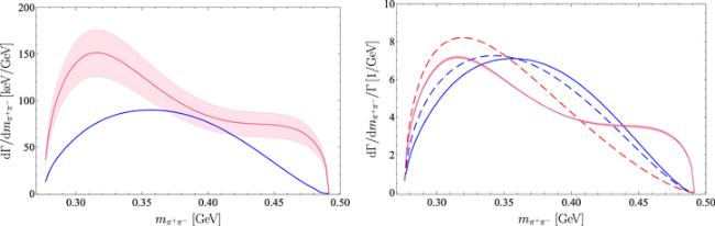
Figure 3. Results in scheme I. Left panel: invariant mass distributions of π+π− for the decay of ${D}_{s1}{(2460)}^{+}\to {D}_{s}^{+}{\pi }^{+}{\pi }^{-}$. Right panel: the invariant mass distributions normalized to the corresponding widths. The red solid curves denote the results considering the loop diagrams in figures 1 (a), (b) and (c) with the S-wave ππ FSI. The red dashed line in the right panel corresponds to the one without the FSI effect. The light-red bands are the corresponding theoretical uncertainties propagated from those of the parameters in scheme I. For comparison, the blue solid and dashed lines are the results in the compact state model for the Ds1(2460), i.e. figure 1 (d) with and without the FSI included, respectively. Dashed lines are only present in the right panel. |
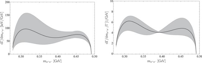
Figure 4. Results in scheme II. Left panel: invariant mass distributions of π+π− for the decay of ${D}_{s1}{(2460)}^{+}\to {D}_{s}^{+}{\pi }^{+}{\pi }^{-}$. Right panel: the invariant mass distributions normalized to the corresponding widths. The black solid curves denote the results by adjusting the subtraction to reproduce the measured ratio in equation ( |
In contrast, if the Ds1(2460) is a compact state which does not couple to D*K, the ππ invariant mass distribution would not receive contributions from the loop diagrams (a), (b) and (c) in figure 1. Then with gc = 7 GeV−1 that is adjusted to produce 13 keV for the partial width of ${D}_{s1}{(2460)}^{+}\to {D}_{s}^{+}{\pi }^{+}{\pi }^{-}$ using equation (16 ), one obtains the blue solid curves in figure 3. The distribution has a broader single bump and takes its maximum at around 0.36 GeV. Switching off the ππ FSI in this case leads to the normalized differential distribution shown as the blue dashed curve in the right panel of figure 3. One sees that the ππ FSI shifts the maximum of the bump to a higher energy.
Therefore, a high statistics measurement of the ππ invariant mass distribution from ${D}_{s1}{(2460)}^{+}\to {D}_{s}^{+}{\pi }^{+}{\pi }^{-}$ would provide one with direct access to the molecular component of the Ds1(2460).
3.2. Predictions on ${B}_{s1}^{0} \rightarrow {B}_{s}^{0}{\pi }^{+}{\pi }^{-}$
Employing heavy quark flavor symmetry, we can make predictions on the decay ${B}_{s1}\to {B}_{s}^{0}{\pi }^{+}{\pi }^{-}$, where Bs1 is the bottom partner of the Ds1(2460). The Bs1 has been predicted in the hadronic molecular model as an isoscalar ${B}^{* }\bar{K}$ bound state [8, 11, 33, 43, 64, 65]. The predicted mass (5774 ± 13) MeV [43] is in accordance with the lattice result on the lowest Bs1 meson (5750 ± 17 ± 19) MeV [66] and slightly larger than the more recent lattice determination of (5741 ± 14) MeV [67]. So far, the only experimentally observed Bs1 meson is the Bs1(5830)0 [3], which is the bottom partner of the Ds1(2536) and not of the one discussed here.
Here, we predict the partial width of the ${B}_{s1}^{0}\to {B}_{s}^{0}{\pi }^{+}{\pi }^{-}$ and the corresponding π+π− invariant mass distribution. The Bs1 is treated as a ${B}^{* }\bar{K}$ molecular state, and the framework is the same as that for the Ds1 in section 3.1 . We take scheme II with the contact term fixed from reproducing the measured ratio in the charm sector in equation (1 ). Heavy quark flavor symmetry requires the contact term coupling in the bottom sector to take a value given by that in equation (23 ) multiplied by $\sqrt{{M}_{{B}_{s1}}{M}_{{B}_{s}}/({M}_{{D}_{s1}}{M}_{{D}_{s}})}$. The ${B}_{s1}{B}^{* }\bar{K}$ coupling is related to that of the Ds1D*K as well, and we use $f={22.5}_{-1.5}^{+1.3}$ GeV from the UChPT results in [43].
Taking 5774 MeV [43] as the Bs1 mass, the partial width of the ${B}_{s1}^{0}\to {B}_{s}^{0}{\pi }^{+}{\pi }^{-}$ is predicted to be
$\begin{eqnarray}{\rm{\Gamma }}({B}_{s1}^{0}\to {B}_{s}^{0}{\pi }^{+}{\pi }^{-})=(3\pm 1)\,\mathrm{keV}.\end{eqnarray}$
The predicted π+π− invariant mass distribution and the one normalized to the above partial width are shown in the left and right panels of figure 5, respectively.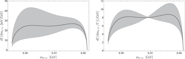
Figure 5. The invariant mass distributions of π+π− for the decay of ${B}_{s1}^{0}\to {B}_{s}^{0}{\pi }^{+}{\pi }^{-}$. Notations are the same as figure 4. |
4. Summary
In this paper, we have calculated the decay width of the ${D}_{s1}(2460)\to {D}_{s}^{+}{\pi }^{+}{\pi }^{-}$ under the assumption that the Ds1(2460) is an isoscalar D*K hadronic molecule. The S-wave ππ final state interaction is taken into account using a dispersive approach. We find that the ratio of partial decays widths ${\rm{\Gamma }}({D}_{s1}(2460)\to {D}_{s}^{+}{\pi }^{+}{\pi }^{-})/{\rm{\Gamma }}({D}_{s1}(2460)\to {D}_{s}^{* +}{\pi }^{0})$ in the molecular picture agrees with the measured value, which may be regarded as a support of the D*K molecular picture for the Ds1(2460). Although the decay ${D}_{s1}(2460)\to {D}_{s}^{+}{\pi }^{+}{\pi }^{-}$ can proceed preserving isospin symmetry while the decay ${D}_{s1}(2460)\to {D}_{s}^{* +}{\pi }^{0}$ violates isospin symmetry, the former has a smaller width due to the three-body phase space suppression.
We also find that the π+π− invariant mass distribution of the decay ${D}_{s1}(2460)\to {D}_{s}^{+}{\pi }^{+}{\pi }^{-}$ can be used to disentangle models for the Ds1(2460). In the D*K molecular picture, the distribution has a double bump structure, due to the D*K loop diagrams and ππ FSI, while in the compact state picture, in which the Ds1D*K coupling is negligible, the distribution has a single broad bump. The π+π− invariant mass distribution can be measured at the LHCb and Belle II experiments.
Furthermore, we also make predictions for the decay ${B}_{s1}^{0}\to {B}_{s}^{0}{\pi }^{+}{\pi }^{-}$ where the ${B}_{s1}^{0}$ is the bottom partner of the Ds1(2460). The partial width is predicted to be (3 ± 1) keV. The ${B}_{s1}^{0}$ may be searched for at the LHCb experiment.
Acknowledgments
This work is supported in part by the National Natural Science Foundation of China (NSFC) and the Deutsche Forschungsgemeinschaft (DFG) through the funds provided to the Sino-German Collaborative Research Center TRR110 ‘Symmetries and the Emergence of Structure in QCD’ (NSFC Grant No. 12070131001, DFG Project-ID 196253076); by the Chinese Academy of Sciences (CAS) under Grant No. XDB34030000; by the NSFC under Grants Nos. 12125507, 11835015, and 12047503; by CAS through the President's International Fellowship Initiative (PIFI) (Grant No. 2018DM0034); and by the VolkswagenStiftung (Grant No. 93562).