Welcome to visit Communications in Theoretical Physics,
Particle Physics and Quantum Field Theory

Neutrino mixing matrix and masses from a particular two-zero texture based on A4 symmetry

  • N Razzaghi
Expand
  • Department of Physics, Qazvin Branch, Islamic Azad University, Qazvin, Iran

Received date: 2022-12-20

  Revised date: 2023-03-28

  Accepted date: 2023-04-05

  Online published: 2023-05-18

Copyright

© 2023 Institute of Theoretical Physics CAS, Chinese Physical Society and IOP Publishing

Abstract

The current study aims to investigate the particular case of two zeros in a Majorana neutrino mass matrix based on A4 symmetry, where charged lepton mass matrix is diagonal. The texture is ${M}_{\nu }^{{S}_{7}}$ with (μ, μ) and (τ, τ) vanishing element of the neutrino mass matrix. The texture ${M}_{\nu }^{{S}_{7}}$ has magic and μτ symmetry, with a tribimaximal form of the mixing matrix, which leads to θ13 = 0 that it is not consistent with experimental data and at first, does not seem to be allowed. Since θ13 a small mixing angle compared to others neutrino mixing angles justifies the use of perturbation theory. We propose that, θ13, and the Dirac phase δ, and two Majorana phases ρ and σ could be generated by using a complex symmetric perturbation mass matrix in the mass basis and find that $\delta {m}^{2}\equiv \,{m}_{2}^{2}-{m}_{1}^{2}\ne 0$ affect to the atmospheric mixing angle. We show that only the predictions of the case I, with Δ < 0 and ${\rm{Re}}(\alpha )\lt 0$, are consistent with the experimental data. Furthermore, the allowed range of our parameter space and complex elements of perturbation mass matrix are found, which led to finding the allowed region of the neutrino masses, the Majorana phases, the effective neutrino mass for the neutrinoless double beta decay, the allowed deviation of θ23 from 45°, and to predict the normal neutrino mass hierarchy. The predicted region of $\langle {m}_{{\nu }_{\beta \beta }}\rangle $ and θ23 are in line with the current experimental data which indicate the accuracy of our model and its results. The results of the case II, with Δ > 0 and ${\rm{Re}}(\alpha )\gt 0$, are ruled out.

Cite this article

N Razzaghi . Neutrino mixing matrix and masses from a particular two-zero texture based on A4 symmetry[J]. Communications in Theoretical Physics, 2023 , 75(5) : 055204 . DOI: 10.1088/1572-9494/acca73

1. Introduction

In the last two decades, neutrino experiments have illustrated that neutrinos oscillate and are massive. Nevertheless, according to the standard parametrization, the unitary lepton mixing matrix, which connects the neutrino mass eigenstates to flavor eigenstates is given by [13]
$\begin{eqnarray}\begin{array}{l}{U}_{\mathrm{PMNS}}=\,\left(\begin{array}{ccc}{c}_{12}{c}_{13} & {s}_{12}{c}_{13} & {s}_{13}{{\rm{e}}}^{-{\rm{i}}\delta }\\ -{s}_{12}{c}_{23}-{c}_{12}{s}_{23}{s}_{13}{{\rm{e}}}^{{\rm{i}}\delta } & {c}_{12}{c}_{23}-{s}_{12}{s}_{23}{s}_{13}{{\rm{e}}}^{{\rm{i}}\delta } & {s}_{23}{c}_{13}\\ {s}_{12}{s}_{23}-{c}_{12}{c}_{23}{s}_{13}{{\rm{e}}}^{{\rm{i}}\delta } & -{c}_{12}{s}_{23}-{s}_{12}{c}_{23}{s}_{13}{{\rm{e}}}^{{\rm{i}}\delta } & {c}_{23}{c}_{13}\end{array}\right)\\ \,\times \,\left(\begin{array}{ccc}1 & 0 & 0\\ 0 & {{\rm{e}}}^{{\rm{i}}\rho } & 0\\ 0 & 0 & {{\rm{e}}}^{{\rm{i}}\sigma }\end{array}\right),\end{array}\end{eqnarray}$
where ${c}_{{ij}}\equiv \cos {\theta }_{{ij}}\mathrm{and}{s}_{{ij}}\equiv \sin {\theta }_{{ij}}$ (for i, j = (1, 2), (1, 3) and (2, 3)); δ is called the Dirac phase, analogous to the CKM phase and ρ, σ are called the Majorana phases, which are relevant for the Majorana neutrinos.
Finally, consequences of the neutrino experiments, such as T2K [4, 5], RENO [6], DOUBLE-CHOOZ [7], and DAYA-BAY [8, 9] have indicated that there are a nonzero mixing angle θ13 which is small compared to the other two mixing angles and a possible nonzero Dirac CP-violation phase δCP. Therefore, the Tribimaximal (TBM) mixing matrix is rejected [10, 11]. The TBM mixing matrix is [12]
$\begin{eqnarray}{U}_{\mathrm{TBM}}=\left(\begin{array}{ccc}\sqrt{\frac{2}{3}} & \frac{1}{\sqrt{3}} & 0\\ \frac{-1}{\sqrt{6}} & \frac{1}{\sqrt{3}} & \frac{1}{\sqrt{2}}\\ \frac{-1}{\sqrt{6}} & \frac{1}{\sqrt{3}} & \frac{-1}{\sqrt{2}}\end{array}\right),\end{eqnarray}$
where, regardless of the model, the mixing angles are: θ12 ≈ 35.26, θ13 ≈ 0, and θ23 ≈ 45° [13].
Before this observation, models leading to the TBM mixing matrix, widely studied [14, 15]. Therefore, to produce θ13 ≠ 0 starting from an initial TBM mixing matrix, different approaches have been adopted [16]. One of the successful phenomenological neutrino mass models with flavor symmetry, which is an appropriate framework for understanding the family structure of charged-lepton and neutrino mass matrices [17, 18], is illustrated by group A4 [1927]. The A4 is a symmetry group of the tetrahedron, was initially presented to illustrate the TBM mixing matrix [21]. Although the primary initial objective of the A4 models was illustrating the TBM mixing matrix [21], many efforts, e.g. [19, 20, 2233], have been made to set up a model capable of describing the non-TBM mixing matrix phenomenology.
The present 3σ global fits for the existing and known neutrino oscillation parameters [34]
$\begin{eqnarray}\begin{array}{rcl}\delta {m}^{2}[{10}^{-5}{{\rm{eV}}}^{2}] & = & (6.94-8.14),\\ | {\rm{\Delta }}{m}^{2}| [{10}^{-3}{{\rm{eV}}}^{2}] & = & (2.47-2.63)-(2.37-2.53),\\ {\sin }^{2}{\theta }_{12} & = & (0.271-0.369),\\ {\sin }^{2}{\theta }_{23} & = & (0.434-0.610)-(0.433-0.608),\\ {\sin }^{2}{\theta }_{13} & = & (0.02000-0.02405)\\ & & -(0.02018-0.02424),\\ \delta & = & (128^\circ -359^\circ )-(200^\circ -353^\circ ),\end{array}\end{eqnarray}$
multiple sets of allowed ranges are stated, and the left and the right columns correspond to normal hierarchy and inverted hierarchy, respectively. $\delta {m}^{2}\equiv {m}_{2}^{2}-{m}_{1}^{2}$ and ${\rm{\Delta }}{m}^{2}\,\equiv {m}_{3}^{2}-{m}_{1}^{2}$.
Despite the prevailing information about neutrino oscillation parameters equation (1.3), the mass and mixing problem in the lepton sector is still conceived as a fundamental problem.
In the current work, we mainly focused on the neutrinos based on the particular case of two-zero textures with A4 symmetry which we called it ${M}_{\nu }^{{S}_{7}}$ [35]. In [35], we have studied all seven possible two-zero textures with A4 symmetry, among which only two textures, the texture with (e, e) and (e, μ) vanishing element of mass matrix and its permutation symmetry, are consistent with the experimental data in the non-perturbation method.
In this paper, we intend to consider ${M}_{\nu }^{{S}_{7}}$ in perturbation method to generate (I) non-zero θ13, (II) CP violation phases δ along with two Majorana phases (ρ and σ) and (III) the deviation of θ23 from 45°. However, the discovery of the θ13, whose smallness (in comparison to other mixing angles) signifies modifying the neutrino mixing matrix using a small perturbation about the basic TBM mixing matrix. By employing different methods in a wide range of contexts, a lot of attempts have been made to generate some of the neutrino parameters in perturbation theory [36].
In the basis where the charged-lepton mass matrix is diagonal, a particular application of A4 is given by [18]
$\begin{eqnarray}{{ \mathcal M }}_{\nu }=\left(\begin{array}{ccc}a+\displaystyle \frac{2d}{3} & b-\displaystyle \frac{d}{3} & c-\displaystyle \frac{d}{3}\\ b-\displaystyle \frac{d}{3} & c+\displaystyle \frac{2d}{3} & a-\displaystyle \frac{d}{3}\\ c-\displaystyle \frac{d}{3} & a-\displaystyle \frac{d}{3} & b+\displaystyle \frac{2d}{3}\end{array}\right),\end{eqnarray}$
which also has magic symmetry.1(1 Magic symmetry is a symmetry in which the sum of elements in either any rows or any columns of the neutrino mass matrix are identical [37].)
Various phenomenological textures, specifically texture zeros [3847], have been investigated in both flavor and non-flavor bases. Such texture zeros not only cause a reduction in the number of free parameters of the neutrino mass matrix, but also contributes to establishing several simple and interesting relations between the parameters of mixing matrix. Therefore, in the current research, this allowed us to explore the effects of a specific case of two-zero texture on ${{ \mathcal M }}_{\nu }$ given by equation (1.4).
Moreover, assuming the Majorana nature of neutrinos, the present study strove to investigate the phenomenological implications of a specific case of two-zero texture of neutrino mass matrix along with A4 symmetry, based on a global fit of neutrino experimental data [34]. This special case of two-zero texture is ${M}_{\nu }^{{S}_{7}}$ with (μ, μ) = (τ, τ) = 0, which can expose the impressive phenomenological features of a defined Majorana neutrino mass matrix.
Our paper is hence organized as follows: in section 2, the methodology is elaborated in two subsections. In subsection A, we reconstruct ${M}_{\nu }^{{S}_{7}}$ in the flavor basis as an unperturbed neutrino mass matrix, and also obtain the unperturbed neutrino mass matrix in the mass basis. In subsection 2.2, we will propose the perturbed neutrino mass matrix as a complex symmetric non-Hermitian matrix in the mass basis. The first order of neutrino mass corrections and the third mass eigenstate are obtained in the mass basis to the first order corrections. Therefore, R&ngr; and the neutrino masses can be expressed. The first two flavor eigenstates are obtained by using the degenerate perturbation method and ∣&ngr;3⟩ in the flavor basis is rewritten. We find the mixing matrix corresponding to our model and thereby ${\sin }^{2}{\theta }_{13}$, CP violation phases (δ, ρ, and σ) and ${\tan }^{2}{\theta }_{23}$ are obtained. In section 3, we compare the results of our work with those of the experimental data in two different cases. In each case, the complex elements of perturbation, α and β, are illustrated onto the allowed region of the parameter space and the allowed regions were found. In case I, where our parameter space and α are negative, the allowed regions of α and β are acceptable; therefore, the predicted regions of $\langle {m}_{{\nu }_{\beta \beta }}\rangle $ and θ23 are obtained which are consistent with the current experimental data and demonstrate the accuracy of our work. In case II, where our parameter space and α are positive, the obtained region of β is not acceptable; therefore the results of case II are ruled out. In section 4, the conclusions are provided.

2. Methodology

2.1. The unperturbed neutrino mass matrix

Assuming the Majorana nature of neutrinos, the mass matrix ${{ \mathcal M }}_{\nu }$ is a complex symmetric matrix in equation (1.4). We examine in [35] the analysis of two-zero texture for the Majorana neutrino mass matrix based on A4 symmetry, ${{ \mathcal M }}_{\nu }$ in equation (1.4), that restricts the number of probably viable cases to seven. It is found that only the texture with (e, e) and (e, μ) vanishing elements of ${{ \mathcal M }}_{\nu }$ and its permutation symmetry, are consistent with the experimental data in the non-perturbation method. The texture with (e, τ) = (μ, μ) = 0, the texture with (e, μ) = (μ, μ) = 0 and their permutation symmetry, are not consistent with the experimental data at all in [35]. The seventh probably viable case of the two-zero texture of ${{ \mathcal M }}_{\nu }$ in with (μ, μ) = (τ, τ) = 0 is extremely interesting. We call it ${M}_{\nu }^{{S}_{7}}$ in [35] and is given by
$\begin{eqnarray}{M}_{\nu }^{{S}_{7}}=\left(\begin{array}{ccc}a+\displaystyle \frac{2}{3}d & -d & -d\\ -d & 0 & a-\displaystyle \frac{d}{3}\\ -d & a-\displaystyle \frac{d}{3} & 0\end{array}\right).\end{eqnarray}$
${M}_{\nu }^{{S}_{7}}$ in equation (2.1) is a magic matrix, which has μτ symmetry [48]. Consequently, it can lead to a TBM mixing matrix in equation (1.2) with θ13 = 0. Therefore, initially seems that ${M}_{\nu }^{{S}_{7}}$ in equation (2.1) is not allowed texture based on experimental data, but because θ13 is small; we believe that the perturbative treatment is a more accurate method to investigate the texture ${M}_{\nu }^{{S}_{7}}$.
A straightforward diagonalization procedure yields ${U}_{\mathrm{TBM}}^{T}{M}_{\nu }^{{S}_{7}}{U}_{\mathrm{TBM}}={M}_{\mathrm{diag}}^{{S}_{7}}$, where
$\begin{eqnarray}\begin{array}{rcl}{m}_{1} & = & a+\displaystyle \frac{5}{3}d,\\ {m}_{2} & = & a-\displaystyle \frac{4}{3}d,\\ {m}_{3} & = & -a+\displaystyle \frac{1}{3}d,\end{array}\end{eqnarray}$
the mass eigenvalues can be complex; they can be presented positive and real by phase transformation, as (1, eiρ, eiσ) in equation (1.1), which ρ and σ are Majorana phases where neutrino oscillations are independent of them.
We reconstruct ${M}_{\nu }^{{S}_{7}}$ in equation (2.1) by using ${M}_{\nu }={U}_{\mathrm{TBM}}{M}_{\mathrm{diag}}{U}_{\mathrm{TBM}}^{T}$, where M&ngr; is a magic neutrino mass matrix with μτ symmetry. In this reconstruction, we define new parameters, as
$\begin{eqnarray}\begin{array}{rcl}m & \equiv & \displaystyle \frac{\sum {m}_{i}}{3}=\displaystyle \frac{({m}_{1}+{m}_{2}+{m}_{3})}{3},\\ {{\rm{\Delta }}}_{32} & \equiv & ({m}_{3}-{m}_{2}),\\ {{\rm{\Delta }}}_{31} & \equiv & ({m}_{3}-{m}_{1}).\end{array}\end{eqnarray}$
Also, because of the reported experimental results, which have shown δm2 is tiny and greater than zero [34], we approximate Δ31 ≃ Δ32 ≡ Δ. Therefore, the unperturbed mass matrix, the reconstructed ${M}_{\nu }^{{S}_{7}}$, in the flavor basis2(2 We work on a basis where the charged lepton mass matrix is diagonal, and thereby, the lepton mixing matrix is extracted from the neutrino mass matrix.) is
$\begin{eqnarray}{M}_{f\nu }^{0}\simeq \left(\begin{array}{ccc}m-\displaystyle \frac{{\rm{\Delta }}}{3} & 0 & 0\\ 0 & m+\displaystyle \frac{{\rm{\Delta }}}{6} & -\displaystyle \frac{{\rm{\Delta }}}{2}\\ 0 & -\displaystyle \frac{{\rm{\Delta }}}{2} & m+\displaystyle \frac{{\rm{\Delta }}}{6}\end{array}\right).\end{eqnarray}$
Still at this level, the unperturbed neutrino mass matrix ${M}_{f\nu }^{0}$ in equation (2.4) has magic and μτ symmetries and can be diagonalized by UTBM3(3 Magic and μτ symmetries for the mass matrix become synonymous with the tribimaximal mixing matrix [37].) in equation (1.2). The mass spectrum of ${M}_{f\nu }^{(0)}$ is
$\begin{eqnarray}{m}_{1}^{(0)}={m}_{2}^{(0)}=m-\displaystyle \frac{{\rm{\Delta }}}{3},\qquad \mathrm{and}\qquad {m}_{3}^{(0)}=m+\displaystyle \frac{2{\rm{\Delta }}}{3}.\end{eqnarray}$
Here ${m}_{1}^{(0)}$, ${m}_{2}^{(0)}$ and ${m}_{3}^{(0)}$ are real and positive and ${m}_{1}^{(0)}$, and ${m}_{2}^{(0)}$ are the same. Hence, the unperturbed mass matrix in the mass basis is
$\begin{eqnarray}{M}_{\mathrm{mass}}^{0}\simeq \left(\begin{array}{ccc}m-\frac{{\rm{\Delta }}}{3} & 0 & 0\\ 0 & m-\frac{{\rm{\Delta }}}{3} & 0\\ 0 & 0 & m+\frac{2{\rm{\Delta }}}{3}\end{array}\right).\end{eqnarray}$
In the mass basis the eigenstates of the unperturbed neutrino mass matrix M0mass in equation (2.6) are as follows:
$\begin{eqnarray}| {\nu }_{1}^{(0)}\rangle =\left(\begin{array}{c}1\\ 0\\ 0\end{array}\right),\,\,\,\,| {\nu }_{2}^{(0)}\rangle =\left(\begin{array}{c}0\\ 1\\ 0\end{array}\right),\,\,\,\,\,| {\nu }_{3}^{(0)}\rangle =\left(\begin{array}{c}0\\ 0\\ 1\end{array}\right),\end{eqnarray}$
in which the first two mass eigenstates above are degenerate. It is noteworthy that the columns of UTBM in equation (1.2) are the unperturbed flavor eigenstates.
Note that, up to now, the shortcomings are: (i) the absence of solar mass splitting, (ii) the neutrino masses ordering is unknown and (iii) the neutrino mixing matrix which is still UTBM. Thus, the main objective is generating the splitting of ${m}_{1}^{(0)}$, and ${m}_{2}^{(0)}$ by means of a mass perturbation, from which θ13 ≠ 0 and CP violation are also derived. Moreover, CP violation conditions are necessarily mandated in that μτ symmetry should be broken. An interesting question is: after breaking the μτ symmetry, will θ23 = 45° remain valid or not?

2.2. The perturbed neutrino mass matrix and perturbation

In this work, we propose the minimal symmetric perturbation neutrino mass matrix4(4 It could be the minimal form of perturbation mass matrix for magic unperturbed neutrino mass matrix with μτ symmetry where the first two mass eigenvalues are degenerate as we work the general form of it in [49].) in the mass basis as
$\begin{eqnarray}{M}_{\mathrm{mass}}^{\mbox{'}}\simeq {\rm{\Delta }}\left(\begin{array}{ccc}0 & 0 & \beta \\ 0 & \alpha & 0\\ \beta & 0 & 0\end{array}\right).\end{eqnarray}$
The dimensionless perturbation elements i.e. α, β can be real or complex and should be small compared to the elements of unperturbed neutrino mass matrix M0mass in equation (2.6) for a valid perturbation theory.
If ${M}_{\mathrm{mass}}^{\mbox{'}}$ is a complex symmetric non-Hermitian matrix given in equation (2.8), therefore we have to consider ${\left({M}_{\mathrm{mass}}^{0}+{M}_{\mathrm{mass}}^{^{\prime} }\right)}^{\dagger }({M}_{\mathrm{mass}}^{0}+{M}_{\mathrm{mass}}^{{\prime} })$ where we drop a term, which is ${ \mathcal O }({\alpha }^{2},\,{\beta }^{2})$. ${{M}_{\mathrm{mass}}^{0}}^{\dagger }{M}_{\mathrm{mass}}^{0}$ is the unperturbed Hermitian term and its eigenstates are the same as those of M0mass in equation (2.7) and its eigenvalues are ${\left({m}_{1}^{(0)}\right)}^{2}$, ${\left({m}_{2}^{(0)}\right)}^{2}$ and ${\left({m}_{3}^{(0)}\right)}^{2}$, therefore the perturbation term is ${M}_{\mathrm{mass}}^{p}\,={M}_{\mathrm{mass}}^{{0}^{\dagger }}{M}_{\mathrm{mass}}^{{\prime} }+{M}_{\mathrm{mass}}^{{{\prime} }^{\dagger }}{M}_{\mathrm{mass}}^{0}$ and the perturbation matrix is
$\begin{eqnarray}{M}_{\mathrm{mass}}^{p}\simeq {\rm{\Delta }}\,\left(\begin{array}{ccc}0 & 0 & {\rm{Re}}(\beta )(2m+\frac{{\rm{\Delta }}}{3})+{\rm{Im}}(\beta )(-{\rm{\Delta }})\\ 0 & {\rm{Re}}(\alpha )(2m-\frac{2{\rm{\Delta }}}{3}) & 0\\ {\rm{Re}}(\beta )(2m+\frac{{\rm{\Delta }}}{3})+{\rm{Im}}(\beta )({\rm{\Delta }}) & 0 & 0\end{array}\right).\end{eqnarray}$
The first-order corrections to the neutrino masses are obtained from ${m}_{i}^{(1)}{\delta }_{{ij}}=\langle {\nu }_{i}^{(0)}| {M}_{\mathrm{mass}}^{{0}^{\dagger }}{M}_{\mathrm{mass}}^{{\prime} }+{M}_{\mathrm{mass}}^{{{\prime} }^{\dagger }}{M}_{\mathrm{mass}}^{0}| {\nu }_{j}^{(0)}\rangle $. Therefore, by using equation (2.5) and first-order corrections to the neutrino masses, we have
$\begin{eqnarray}\begin{array}{rcl}{m}_{1}^{2} & = & {\left({m}_{1}^{(0)}\right)}^{2},\\ {m}_{2}^{2} & = & {\left({m}_{2}^{(0)}\right)}^{2}+{\rm{Re}}(\alpha )\left(2m-\displaystyle \frac{2}{3}{\rm{\Delta }}\right){\rm{\Delta }},\\ {m}_{3}^{2} & = & {\left({m}_{3}^{(0)}\right)}^{2}.\end{array}\end{eqnarray}$
The mass corrections arise from the first-order corrections with ${m}_{2}^{(1)}\ne 0$, and ${m}_{1}^{(1)}={m}_{3}^{(1)}=0$. Therefore, the splitting of m1, and m2 is equal to ${m}_{2}^{(1)}$. So far, Neutrino experimental data have definitely confirmed that $\delta {m}^{2}={m}_{2}^{2}-{m}_{1}^{2}\gt 0$. Therefore, due to the equation (2.5), ${m}_{2}^{(1)}\,=2{\rm{\Delta }}{\rm{Re}}(\alpha )({m}_{2}^{(0)})$ must be positive.
From mass-squared in equation (2.10), we could obtain the ratio of two neutrino mass-squared differences ${R}_{\nu }=\tfrac{\delta {m}^{2}}{{\rm{\Delta }}{m}^{2}}$, as
$\begin{eqnarray}{R}_{\nu }={\rm{Re}}(\alpha )\displaystyle \frac{6m-2{\rm{\Delta }}}{6m+{\rm{\Delta }}},\end{eqnarray}$
where $\delta {m}^{2}\equiv {m}_{2}^{2}-{m}_{1}^{2}$ and ${\rm{\Delta }}{m}^{2}\equiv {m}_{3}^{2}-{m}_{1}^{2}$.
Moreover, employing equation (2.5), equation (2.10), and equation (2.11) as well as the definitions associated δm2 and Δm2, the neutrino masses can be expressed with more convenient relations. More concretely, m1, m2, and m3 are related to $\tfrac{m}{{\rm{\Delta }}}$, and ${\rm{Re}}(\alpha )$, our parameter space, and the experimental parameters δm2 and R&ngr; as
$\begin{eqnarray}\begin{array}{rcl}{m}_{1} & = & \sqrt{\delta {m}^{2}\,B},\\ {m}_{2} & = & \sqrt{\delta {m}^{2}(B+1)},\\ {m}_{3} & = & \sqrt{\delta {m}^{2}\left(\displaystyle \frac{1}{{R}_{\nu }}+B\right)},\end{array}\end{eqnarray}$
where $B\equiv \tfrac{\tfrac{m}{{\rm{\Delta }}}-\tfrac{1}{3}}{2{\rm{Re}}(\alpha )}$. Therefore, according to equation (2.12), our prediction is normal neutrino mass hierarchy.
It is worth noting that the lowest order of the first two flavor eigenstates in degenerate perturbation theory are
$\begin{eqnarray}| {\nu }_{1}{\rangle }_{\mathrm{flavor}}=\left(\begin{array}{c}\sqrt{\frac{2}{3}}\\ -\frac{1}{\sqrt{6}}\\ -\frac{1}{\sqrt{6}}\end{array}\right)+\left(\begin{array}{c}0\\ \frac{-\left(\frac{3{\rm{i}}{\rm{\Delta }}{\rm{Im}}(\beta )}{6m+{\rm{\Delta }}}+{\rm{Re}}(\beta )\right)}{\sqrt{2}}\\ \frac{\left(\frac{3{\rm{i}}{\rm{\Delta }}{\rm{Im}}(\beta )}{6m+{\rm{\Delta }}}+{\rm{Re}}(\beta )\right)}{\sqrt{2}}\end{array}\right)\end{eqnarray}$
and5(5 $({M}_{\mathrm{mass}}^{0}+{M}_{\mathrm{mass}}^{\mbox{'}})$ has magic symmetry in the flavor basis.)
$\begin{eqnarray}| {\nu }_{2}{\rangle }_{\mathrm{flavor}}=\left(\begin{array}{c}\frac{1}{\sqrt{3}}\\ \frac{1}{\sqrt{3}}\\ \frac{1}{\sqrt{3}}\end{array}\right).\end{eqnarray}$
We reproduce the third mass eigenstate ∣&ngr;3 〉 , in the mass basis, to the first order corrections by
$\begin{eqnarray}| {\nu }_{3}{\rangle }_{\mathrm{mass}}=| {\nu }_{3}^{(0)}\rangle +\frac{\langle {\nu }_{j}^{(0)}| {M}_{\mathrm{mass}}^{p}| {\nu }_{3}^{(0)}\rangle }{{\left({m}_{3}^{(0)}\right)}^{2}-{\left({m}_{j}^{(0)}\right)}^{2}}| {\nu }_{j}^{(0)}\rangle ,\,\,(j\ne 3).\,\end{eqnarray}$
By inserting equation (2.5), equation (2.7), and equation (2.9) into equation (2.15), we obtain ∣&ngr;3mass as
$\begin{eqnarray}| {\nu }_{3}{\rangle }_{\mathrm{mass}}=\left(\begin{array}{c}{\rm{Re}}(\beta )-\frac{3{\rm{i}}{\rm{\Delta }}}{6m+{\rm{\Delta }}}{\rm{Im}}(\beta )\\ 0\\ 1\end{array}\right).\end{eqnarray}$
Now, we rewrite ∣&ngr;3>mass in the flavor basis, as follows
$\begin{eqnarray}| {\nu }_{3}{\rangle }_{\mathrm{flavor}}=\left(\begin{array}{c}\sqrt{\frac{2}{3}}\left(\frac{-3{\rm{i}}{\rm{\Delta }}{\rm{Im}}(\beta )}{6m+{\rm{\Delta }}}+{\rm{Re}}(\beta )\right)\\ \frac{1}{\sqrt{2}}-\frac{\frac{-3{\rm{i}}{\rm{\Delta }}{\rm{Im}}(\beta )}{6m+{\rm{\Delta }}}+{\rm{Re}}(\beta )}{\sqrt{6}}\\ -\frac{1}{\sqrt{2}}-\frac{\frac{-3{\rm{i}}{\rm{\Delta }}{\rm{Im}}(\beta )}{6m+{\rm{\Delta }}}+{\rm{Re}}(\beta )}{\sqrt{6}}\end{array}\right),\end{eqnarray}$
Using degenerate perturbation theory, according to equation (2.13), equation (2.14), and equation (2.17), we obtain the neutrino mixing matrix with δ ≠ 0, as
$\begin{eqnarray}U=\left(\begin{array}{ccc}\sqrt{\displaystyle \frac{2}{3}} & \displaystyle \frac{1}{\sqrt{3}} & \sqrt{\displaystyle \frac{2}{3}}\left(\displaystyle \frac{-3{\rm{i}}{\rm{\Delta }}{\rm{Im}}(\beta )}{6m+{\rm{\Delta }}}+{\rm{Re}}(\beta )\right)\\ -\displaystyle \frac{1}{\sqrt{6}}-\displaystyle \frac{\left(\tfrac{3{\rm{i}}{\rm{\Delta }}{\rm{Im}}(\beta )}{6m+{\rm{\Delta }}}+{\rm{Re}}(\beta )\right)}{\sqrt{2}} & \displaystyle \frac{1}{\sqrt{3}} & \displaystyle \frac{1}{\sqrt{2}}-\displaystyle \frac{\tfrac{-3{\rm{i}}{\rm{\Delta }}{\rm{Im}}(\beta )}{6m+{\rm{\Delta }}}+{\rm{Re}}(\beta )}{\sqrt{6}}\\ -\displaystyle \frac{1}{\sqrt{6}}+\displaystyle \frac{\left(\tfrac{3{\rm{i}}{\rm{\Delta }}{\rm{Im}}(\beta )}{6m+{\rm{\Delta }}}+{\rm{Re}}(\beta )\right)}{\sqrt{2}} & \displaystyle \frac{1}{\sqrt{3}} & -\displaystyle \frac{1}{\sqrt{2}}-\displaystyle \frac{\tfrac{-3{\rm{i}}{\rm{\Delta }}{\rm{Im}}(\beta )}{6m+{\rm{\Delta }}}+{\rm{Re}}(\beta )}{\sqrt{6}}\end{array}\right),\end{eqnarray}$
and
$\begin{eqnarray}{U}_{\mathrm{tot}}=U\times \left(\begin{array}{ccc}1 & 0 & 0\\ 0 & {{\rm{e}}}^{{\rm{i}}\rho } & 0\\ 0 & 0 & {{\rm{e}}}^{{\rm{i}}\sigma }\end{array}\right).\end{eqnarray}$
We calculate the mixing angles from the mixing matrix U in equation (2.18), as follows
$\begin{eqnarray}\begin{array}{rcl}{\sin }^{2}{\theta }_{13} & = & | {U}_{13}{| }^{2}=\displaystyle \frac{1}{A}\left(\displaystyle \frac{2}{3}{\left({\rm{Re}}(\beta )\right)}^{2}+\displaystyle \frac{6{{\rm{\Delta }}}^{2}}{{\left(6m+{\rm{\Delta }}\right)}^{2}}{\left({\rm{Im}}(\beta )\right)}^{2}\right),\\ {\sin }^{2}{\theta }_{12} & = & \displaystyle \frac{| {U}_{12}{| }^{2}}{1-| {U}_{13}{| }^{2}}=\displaystyle \frac{A}{2+A},\\ {\tan }^{2}{\theta }_{23} & = & \displaystyle \frac{| {U}_{23}{| }^{2}}{| {U}_{33}{| }^{2}}=1-\displaystyle \frac{4\sqrt{3}{\rm{Re}}(\beta )}{2+A+2\sqrt{3}{\rm{Re}}(\beta )}.\end{array}\end{eqnarray}$
where $A=1+{\left({\rm{Re}}(\beta )\right)}^{2}+\tfrac{9{{\rm{\Delta }}}^{2}}{{\left(6m+{\rm{\Delta }}\right)}^{2}}{\left({\rm{Im}}(\beta )\right)}^{2}$.
We add the perturbation matrix, ${M}_{\mathrm{mass}}^{\mbox{'}}$ in equation (2.8), in our texture with complex components in the mass basis which leads to the solar neutrino mass splitting, θ13 ≠ 0, the deviation of $\tan {\theta }_{23}$ from 1, nonzero the CP-violating phases (the Dirac phase δ, and two Majorana phases ρ and σ). In the following, a straightforward calculation yields these phases.
As mentioned in the appendix, we could obtain $\tan \delta $ by using the elements of the mixing matrix U in equation (2.18) and the mixing angles in equation (2.20), where we have dropped the terms of ${ \mathcal O }{\left({\rm{Re}}(\beta )\right)}^{2}$ and ${ \mathcal O }{\left({\rm{Im}}(\beta )\right)}^{2}$, as follows
$\begin{eqnarray}\tan \delta =\displaystyle \frac{(-3{\rm{\Delta }}){\rm{Im}}(\beta )}{(6m+{\rm{\Delta }}){\rm{Re}}(\beta )}.\end{eqnarray}$
In the basis where the charged lepton mass matrix is diagonal, by employing ${({M}_{\nu }^{0}+{M}_{\nu }^{\mbox{'}})}_{\mathrm{flavor}}={U}_{{tot}}{({M}_{\nu })}_{\mathrm{diag}}{{U}_{\mathrm{tot}}}^{T}$, we reorganize ${({M}_{\nu }^{0}+{M}_{\nu }^{\mbox{'}})}_{\mathrm{flavor}}$ as
$\begin{eqnarray}{({M}_{\nu }^{0}+{M}_{\nu }^{\mbox{'}})}_{\mathrm{flavor}}=U\left(\begin{array}{ccc}{m}_{1} & 0 & 0\\ 0 & {{\rm{e}}}^{2{\rm{i}}\rho }{m}_{2} & 0\\ 0 & 0 & {{\rm{e}}}^{2{\rm{i}}\sigma }{m}_{3}\end{array}\right){U}^{T},\end{eqnarray}$
where we adopted the mixing matrix U given by equation (2.18), and neutrino masses mi, i = 1, 2, 3 given by equation (2.10).
We obtain six complex equations by using equation (2.22) regarding the elements of neutrino mass matrix, in the flavor basis, at (i, j) positions as follows
$\begin{eqnarray}{m}_{1}{U}_{i1}{U}_{j1}+{{\rm{e}}}^{2{\rm{i}}\rho }{m}_{2}{U}_{i2}{U}_{j2}+{{\rm{e}}}^{2{\rm{i}}\sigma }{m}_{3}{U}_{i3}{U}_{j3}={M}_{{ij}}.\end{eqnarray}$
By inserting the elements of mixing matrix U in equation (2.18) into equation (2.23) and solving dirty math equations, and neglecting terms of ${ \mathcal O }{\left({\rm{Re}}(\beta )\right)}^{2}$ and ${ \mathcal O }{\left({\rm{Im}}(\beta )\right)}^{2}$, we obtain ρ = −σ and the CP-violating Majorana phases ρ and σ are as follows
$\begin{eqnarray}\sin (2\rho )=-\sin (2\sigma )=\displaystyle \frac{12\,{\rm{\Delta }}\,{\rm{Re}}(\beta )\,{\rm{Im}}(\beta )\,{m}_{3}}{({\rm{\Delta }}+6m){m}_{2}}.\end{eqnarray}$
Up to this point, having used the perturbation method, we could obtain (I) the splitting of the two first neutrino masses, (II) the perturbed mass eigenstates in the CP violation case, therefore generating (III) θ13 ≠ 0, (IV) the Dirac phase δ, (V) the deviation rate of θ23 from 45, (VI) the mixing matrix corresponding to our texture, and (VII) the two Majorana phases ρ and σ. In the next section, by comparing the results of our work with those of the experimental data in equation (1.3), we will show that ${M}_{\nu }^{{S}_{7}}$ (2.1) could be allowed texture.

3. Comparison with experimental data

In this section, the results of the current study are compared with those of the experimental data in equation (1.3). As it was mentioned in the previous section, according to neutrino experimental data, we have $\delta {m}^{2}=2\,{\rm{\Delta }}\,{\rm{Re}}(\alpha ){m}_{2}^{(0)}\gt 0$. Therefore, since ${m}_{2}^{(0)}$ in equation (2.5) is real and positive, we have two cases; case (I) Δ and ${\rm{Re}}(\alpha )$ to be negative, case (II) Δ and ${\rm{Re}}(\alpha )$ to be positive.
Initially, we consider case I, when Δ < 0 and ${\rm{Re}}(\alpha )\lt 0$. The investigation of case I includes three steps; in the first step, we obtain the allowed range of ${\rm{Re}}(\alpha )$. We do this by mapping two of the constraints obtained from the experimental data onto our parameter space, $\tfrac{m}{{\rm{\Delta }}}$, as shown in figure 1. The two restricting sets of experimental data on neutrino mass come from the values of ${R}_{\nu }=\tfrac{\delta {m}^{2}}{{\rm{\Delta }}{m}^{2}}$ and ∑m&ngr;6(6m&ngr; < 0.12 eV is the significant experimental result reported by Planck's measurements of the cosmic microwave background (CMB) [50].). The overlap of the experimental data of R&ngr; and ∑m&ngr; and our model, equation (2.11) and equation (2.12), is restricted to a tiny region close to the bottom-right corner of the parameter space in figure 1, where we have magnified the overlap region in the zoomed box.
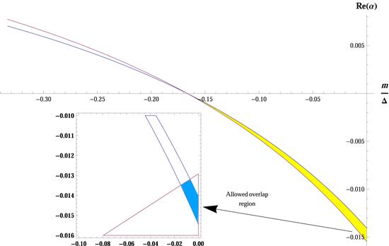
Figure 1. In this figure, the whole region of the ${\rm{Re}}(\alpha )-\tfrac{m}{{\rm{\Delta }}}$ plane which is allowed by our model is shown. The yellow (dark) area below the horizontal axis displays the allowed region of ${\rm{Re}}(\alpha )$ in case I, according to the experimental data of R&ngr;. In the zoomed box, we have magnified the blue (dark) tiny overlap region of the experimental values for R&ngr; and ∑m&ngr;, which is consistent with all of the experimental data.
Therefore, as is shown in the zoomed box in figure 1, we could specify the allowed ranges of our parameter space, $\tfrac{m}{{\rm{\Delta }}}$, and ${\rm{Re}}(\alpha )$ as follows,
$\begin{eqnarray}\displaystyle \frac{m}{{\rm{\Delta }}}\approx \,(-0.015-0).\end{eqnarray}$
$\begin{eqnarray}{\rm{Re}}(\alpha )\approx \,-(0.01350-0.01320)\to \,-(0.01550-0.01405).\end{eqnarray}$
Having determined the unique overlap region in the above, we can predict the masses of the neutrinos in equation (2.12) as follows;
$\begin{eqnarray}\begin{array}{rcl}{m}_{1} & = & \{(0.02992-0.03241),(0.02991-0.03239)\}\,\mathrm{eV}\\ & \to & \,\{(0.02732-0.02959),(0.02869-0.03107)\}\,\mathrm{eV},\\ {m}_{2} & = & \{(0.03106-0.0336),(0.03104-0.03362)\}\,\mathrm{eV}\\ & \to & \{(0.02856-0.03093),(0.02987-0.03235)\}\,\mathrm{eV},\\ {m}_{3} & = & \{(0.05801-0.06066),(0.05800-0.05936)\}\,\mathrm{eV}\\ & \to & \{(0.05671-0.05920),(0.05738-0.05996)\}\,\mathrm{eV}.\end{array}\end{eqnarray}$
In the second step, we obtain the allowed range of $\tfrac{{\rm{Im}}(\beta )}{{\rm{Re}}(\beta )}$, as is shown in the zoomed box in figure 2. We do this by inserting the experimental data of $\tan \delta $ into the equation of $\tan \delta $ in equation (2.21) and mapping $\tfrac{{\rm{Im}}(\beta )}{{\rm{Re}}(\beta )}$ according to the allowed range of our parameter space in equation (3.1).
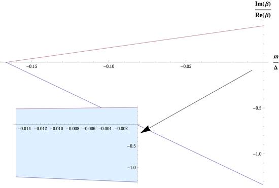
Figure 2. In this figure, the whole region of the $\tfrac{{\rm{Im}}(\beta )}{{\rm{Re}}(\beta )}-\tfrac{m}{{\rm{\Delta }}}$ plane, which displays the region of $\tfrac{{\rm{Im}}(\beta )}{{\rm{Re}}(\beta )}-\tfrac{m}{{\rm{\Delta }}}$ in case I, according to the experimental data of R&ngr; and $\tan \delta $. In the zoomed box, we have magnified the light blue (dark) tiny dark allowed region of the $\tfrac{{\rm{Im}}(\beta )}{{\rm{Re}}(\beta )}$ according to the region of our parameter space, $\tfrac{m}{{\rm{\Delta }}}$ in equation (3.1).
Therefore, we obtain the allowed region of $\tfrac{{\rm{Im}}(\beta )}{{\rm{Re}}(\beta )}$ onto our parameter space which is consistent with the experimental data as follows
$\begin{eqnarray}\displaystyle \frac{{\rm{Im}}(\beta )}{{\rm{Re}}(\beta )}\approx ((-1.21)-0.35)\to ((-1.31)-0.4),\end{eqnarray}$
accordingly, can write
$\begin{eqnarray}{\rm{Im}}(\beta )\approx ((-1.21)-0.35){\rm{Re}}(\beta )\to ((-1.31)-0.4){\rm{Re}}(\beta ),\end{eqnarray}$
therefore in the second step, we obtain the ratio of $\tfrac{{\rm{Im}}(\beta )}{{\rm{Re}}(\beta )}$.
In the third step, we obtain the allowed range of ${\rm{Re}}(\beta )$, as is shown in the zoomed box in figure 3, and subsequently the allowed range of ${\rm{Im}}(\beta )$ due to equation (3.5). We do this by inserting the experimental data of ${\sin }^{2}{\theta }_{13}$ into the first equation of equation (2.20) and mapping ${\rm{Re}}(\beta )$ onto the allowed range of our parameter space in equation (3.1).
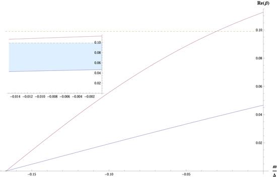
Figure 3. In this figure, the whole region of the ${\rm{Re}}(\beta )-\tfrac{m}{{\rm{\Delta }}}$ plane, which displays the region of ${\rm{Re}}(\beta )-\tfrac{m}{{\rm{\Delta }}}$ in case I, according to the experimental data of R&ngr; and ${\sin }^{2}{\theta }_{13}$. In the zoomed box, we have magnified the light blue (dark) tiny allowed region of the ${\rm{Re}}(\beta )$, below the line 0.099, according to the region of our parameter space, $\tfrac{m}{{\rm{\Delta }}}$ in equation (3.1).
According to perturbation theory, the perturbation elements i.e. α, and β in equation (2.8) should be small compared to the elements of unperturbed neutrino mass matrix m, and Δ in equation (2.6). Accordingly, we only accept those values of ${\rm{Re}}(\beta )$ that are less than 0.1.7(7 We choose ${\rm{Re}}(\beta )\lt 0.1$ because of the important experimental result for the sum of the three light neutrino masses that have been reported by the Planck measurements of the cosmic microwave background, which is ∑m&ngr; < 0.12 eV [50].) Therefore, the tiny region below the line 0.099 in the zoomed box in figure 3 displays the allowed region of ${\rm{Re}}(\beta )$ according to the allowed range of our parameter space, as
$\begin{eqnarray}{\rm{Re}}(\beta )\approx \,(0.05057-0.099)\to (0.046-0.099).\end{eqnarray}$
In the following, based on equation (3.5), and equation (3.6) the allowed region of ${\rm{Im}}(\beta )$ is obtained, as follows
$\begin{eqnarray}{\rm{Im}}(\beta )\approx \,((-0.099)-(0.0177))\to ((-0.099)-(0.0184)),\end{eqnarray}$
Having taken these three steps, we obtained the allowed region of our parameter space, $\tfrac{m}{{\rm{\Delta }}}$ in equation (3.1), and dimensionless perturbation elements ${\rm{Re}}(\alpha )$, ${\rm{Re}}(\beta )$, and ${\rm{Im}}(\beta )$, respectively in equation (3.2), equation (3.6), and equation (3.7).
Let us now proceed with our discussions by obtaining the range of predicted values of Majorana phases in case I for the texture ${M}_{\nu }^{{S}_{7}}$.
By taking $\tfrac{m}{{\rm{\Delta }}}$, ${\rm{Re}}(\beta )$, and ${\rm{Im}}(\beta )$ from equation (3.1), equation (3.6), and equation (3.7) respectively, our herein model yields the following values for the Majorana phases ρ and σ:
$\begin{eqnarray}\rho =-\sigma \approx \,((-3.50^\circ )-(1.24^\circ ))\to ((-3.11^\circ )-(1.19^\circ )),\end{eqnarray}$
which may be tested by future experiments.
In the following, we outline further predictions of our model in case I, which can be a test of the accuracy of our predictions.

The Majorana neutrinos can violate lepton number for example in the neutrinoless double beta decay procedure (ββ0&ngr;) [51]. Such a process has not been detected yet, but an upper bound has been set for the relevant quantity, i.e. $\langle {m}_{{\nu }_{\beta \beta }}\rangle $. Results from the first phase of the KamLAND-Zen experiment sets the following constraint $\langle {m}_{{\nu }_{\beta \beta }}\rangle \lt (0.061-0.165)\,\mathrm{eV}$ at 90 present CL [52]. The prediction of our model for $\langle {m}_{{\nu }_{\beta \beta }}\rangle $ is:

$\begin{eqnarray}\langle {m}_{{\nu }_{\beta \beta }}\rangle \approx \,(0.02642-0.03264)\to (0.02332-0.03146)\,\mathrm{eV},\end{eqnarray}$
which consistent with the result of kamLAND-Zen experiment.

The value of ${\tan }^{2}{\theta }_{23}$ can be obtained by inserting equation (3.1), equation (3.6), and equation (3.7) into equation (2.20). Let us plot ${\tan }^{2}{\theta }_{23}$ according to equation (2.20), based on the allowed region of perturbation elements, onto allowed region of parameter space, as is shown in the zoomed box in figure 4. Interestingly, the values obtained for ${\tan }^{2}{\theta }_{23}$ corroborate those of with the experimental data in equation (1.3). We find the allowed region of θ23 in case I as follows

$\begin{eqnarray}{\theta }_{23}\approx (41.80^\circ -43.47^\circ ),\end{eqnarray}$
which indicates the accuracy of predictions of the case I in our work.

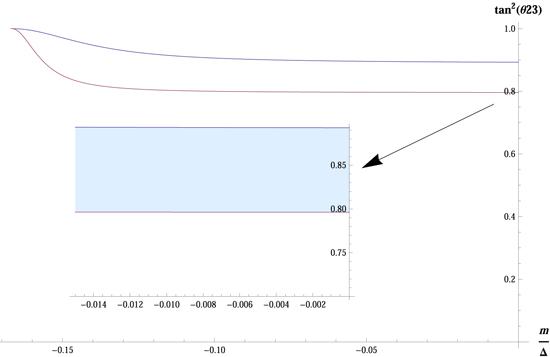
Figure 4. In this figure, the whole region of the ${\tan }^{2}{\theta }_{23}-\tfrac{m}{{\rm{\Delta }}}$ plane, which displays the region of ${\tan }^{2}{\theta }_{23}-\tfrac{m}{{\rm{\Delta }}}$ in case I, according to the experimental data of R&ngr; and ${\tan }^{2}{\theta }_{23}$. In the zoomed box, we have magnified the light blue (dark) tiny allowed region of the ${\tan }^{2}{\theta }_{23}$, according to the region of our parameter space $\tfrac{m}{{\rm{\Delta }}}$ in equation (3.1), which is in complete agreement with the experimental data in equation (1.3).
Now we consider our work according to case II when Δ and ${\rm{Re}}(\alpha )$ are both positive. In this case, similar to case I, we first obtain the allowed range of ${\rm{Re}}(\alpha )$ as is shown in the zoomed box in figure 5. We do this by mapping R&ngr; and ∑m&ngr;, two of the constraints obtained from the experimental data onto our parameter space8(8 At first glance, it seems that the allowed region of the parameter space in case II is $\tfrac{m}{{\rm{\Delta }}}\geqslant \tfrac{1}{3}$ which is obtained based on δ m2 > 0.) of case II, according to the experimental data in equation (1.3). The overlap of the experimental data of R&ngr; and ∑m&ngr; and our model, equation (2.11) and equation (2.12), is restricted to a tiny region inside the right triangle, which is shown in the zoomed box in figure 5.
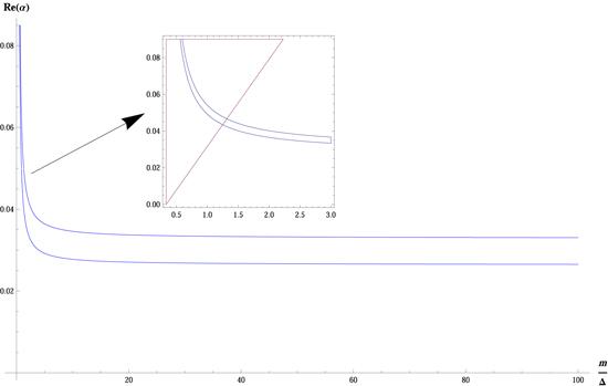
Figure 5. In this figure, the whole region of the ${\rm{Re}}(\alpha )-\tfrac{m}{{\rm{\Delta }}}$ plane which is allowed by our model in the case II is shown. The area between the two blue curves displays the allowed region of ${\rm{Re}}(\alpha )$ in case II, according to the experimental data of R&ngr;. In the zoomed box, we have magnified a tiny overlap region of the experimental values for R&ngr; and ∑m&ngr; inside right triangle.
Therefore in case II, as is shown in the zoomed box in figure 5, we could specify the allowed ranges of our parameter space, $\tfrac{m}{{\rm{\Delta }}}$, and ${\rm{Re}}(\alpha )$ as follows,
$\begin{eqnarray}\displaystyle \frac{m}{{\rm{\Delta }}}\approx \,(0.56-1.3).\end{eqnarray}$
$\begin{eqnarray}{\rm{Re}}(\alpha )\approx \,(0.042-0.09).\end{eqnarray}$
In the next step, we obtain the allowed range of $\tfrac{{\rm{Im}}(\beta )}{{\rm{Re}}(\beta )}$ in case II as is shown in the zoomed box in figure 6. The same is case I, we do this by inserting the experimental data of $\tan \delta $ into the equation of $\tan \delta $ in equation (2.21) and mapping $\tfrac{{\rm{Im}}(\beta )}{{\rm{Re}}(\beta )}$ according to the allowed range of our parameter space in equation (3.11).
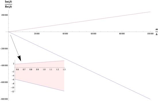
Figure 6. In this figure, the whole region of the $\tfrac{{\rm{Im}}(\beta )}{{\rm{Re}}(\beta )}-\tfrac{m}{{\rm{\Delta }}}$ plane, which displays the region of $\tfrac{{\rm{Im}}(\beta )}{{\rm{Re}}(\beta )}-\tfrac{m}{{\rm{\Delta }}}$ in case II, according to the experimental data of R&ngr; and $\tan \delta $. In the zoomed box, we have magnified the light pink (dark) tiny allowed region of the $\tfrac{{\rm{Im}}(\beta )}{{\rm{Re}}(\beta )}$ according to the region of our parameter space, $\tfrac{m}{{\rm{\Delta }}}$ in equation (3.11).
We obtain that the allowed region of $\tfrac{{\rm{Im}}(\beta )}{{\rm{Re}}(\beta )}$ onto our parameter space, in case II, as
$\begin{eqnarray}\displaystyle \frac{{\rm{Im}}(\beta )}{{\rm{Re}}(\beta )}\approx \,(-(12)-3.4),\end{eqnarray}$
therefore, according to equation (3.13) we could write
$\begin{eqnarray}{\rm{Im}}(\beta )\approx \,(-(12)-3.4){\rm{Re}}(\beta ).\end{eqnarray}$
we obtain the allowed range of ${\rm{Re}}(\beta )$, as is shown in the zoomed box in figure 7. As in case I, We do this by inserting the experimental data of ${\sin }^{2}{\theta }_{13}$ into the first equation of equation (2.20) and mapping ${\rm{Re}}(\beta )$ onto the allowed range of our parameter space of case II.
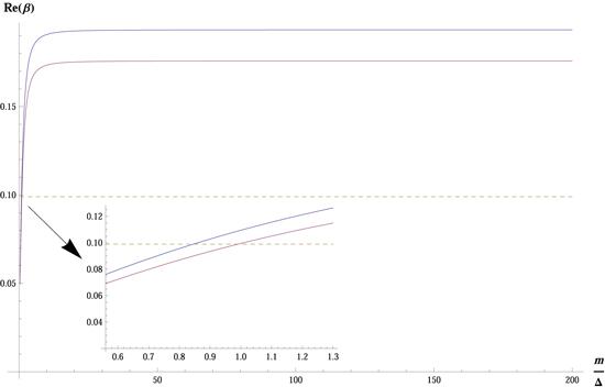
Figure 7. In this figure, the whole region of the ${\rm{Re}}(\beta )-\tfrac{m}{{\rm{\Delta }}}$ plane, which displays the region of ${\rm{Re}}(\beta )-\tfrac{m}{{\rm{\Delta }}}$ in case II, according to the experimental data of R&ngr; and ${\sin }^{2}{\theta }_{13}$. In the zoomed box, we have magnified a tiny allowed region of the ${\rm{Re}}(\beta )$, below the line 0.099, according to the region of our parameter space, $\tfrac{m}{{\rm{\Delta }}}$ in equation (3.11).
As mentioned in the previous case, the allowed range of ${\rm{Re}}(\beta )$ must be below 0.099; therefore, the area between two curves below the horizontal dashed line in the zoomed box in figure 7 displays the allowed range of ${\rm{Re}}(\beta )$ in case II as follows,
$\begin{eqnarray}{\rm{Re}}(\beta )\approx \,(0.07-0.099).\end{eqnarray}$
Afterwards, we map ${\rm{Im}}(\beta )$ based on equation (3.14) and equation (3.14), as is shown in the two figure 8 and, figure 9. We find that in case II the obtained value of ${\rm{Im}}(\beta )$ is much greater than ∣0.1∣, the red dashed line, which is not acceptable by the perturbation theory. Therefore, the obtained results in case II, with Δ > 0 and ${\rm{Re}}(\alpha )\gt 0$, are ruled out.
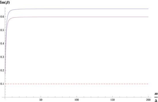
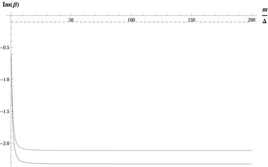
Figure 8. In this figure, the whole region of the ${\rm{Im}}(\beta )-\tfrac{m}{{\rm{\Delta }}}$ plane, which displays the region of ${\rm{Im}}(\beta )-\tfrac{m}{{\rm{\Delta }}}$ in case II, according to the value of ${\rm{Re}}(\beta )$ in equation (3.15) and when ${\rm{Im}}(\beta )$ in equation (3.15) is chosen from the positive region. The value of ${\rm{Im}}(\beta )$ is not acceptable within our model because is greater than ∣0.1∣ (the red dashed line).
Figure 9. In this figure, the whole region of the ${\rm{Im}}(\beta )-\tfrac{m}{{\rm{\Delta }}}$ plane, which displays the region of ${\rm{Im}}(\beta )-\tfrac{m}{{\rm{\Delta }}}$ in case II, according to the value of ${\rm{Re}}(\beta )$ in equation (3.15) and when ${\rm{Im}}(\beta )$ in equation (3.15) is chosen from the negative region. The value of ${\rm{Im}}(\beta )$ is not acceptable within our model because is greater than ∣0.1∣ (the red dashed line).

4. Conclusion

In assessing neutrino physics from a phenomenological point of view, the texture of the neutrino mass matrix is of particular relevance. The choice of symmetries for the mass matrix can lead to specific states in the mixing matrix, which may convey results consistent with the corresponding experimental data. Such consequences are significant because we can make additional predictions regarding neutrinos and their flavor symmetries.
One salient feature of investigating the neutrino mass matrix phenomena is that it could provide new indications for understanding the flavor symmetry and symmetry breaking simultaneously. Therefore, these symmetries and maybe the breaking of them could impact the neutrino mixing matrix, which has significant differences in the magnitude of (mixing) angles in contrast to the quark sector. Furthermore, studying the texture of the neutrino mass matrix could predict the answer to the following essential questions: (a) what are the masses of neutrinos? (b) what is the ordering of the three neutrino masses? (c) neutrinos are Dirac or Majorana Particles? (d) what are the values of three CP-violating phases of the PMNS mixing matrix? (e) how close to $\tfrac{\pi }{4}$ is θ23? (f) Do sterile neutrinos exist? certainly, these questions will be solved by future experiments.
In this work, by proposing a particular two-zero texture based on A4 symmetry along with magic and μτ symmetry, we have obtained predictions for all the previous questions that are consistent with the current experimental data.
We have studied the phenomenology of two-zero texture in the Majorana neutrino mass matrix along with A4 symmetry where the charged lepton mass matrix is diagonal. Therefore, there are seven possible two-zero textures. The seven viable textures are broadly categorized into two categories. To sum up, in general, textures which are consistent with the experimental data as ${M}_{\nu }^{{S}_{1}}$, ${M}_{\nu }^{{S}_{2}}$, ${M}_{\nu }^{{S}_{7}}$ and textures which are not consistent with the experimental data as ${M}_{\nu }^{{S}_{3}}$, ${M}_{\nu }^{{S}_{5}}$, and their permutation symmetry, as ${M}_{\nu }^{{S}_{4}}$, ${M}_{\nu }^{{S}_{6}}$ respectively.9(9 We have studied the texture ${M}_{\nu }^{{S}_{1}}$ and its permutation symmetry as texture ${M}_{\nu }^{{S}_{2}}$ in the non-perturbation method and find results that are exactly consistent with the experimental data. We also find that textures ${M}_{\nu }^{{S}_{3}}$, ${M}_{\nu }^{{S}_{5}}$ and their permutation symmetry are ruled out [35].)
In our work, We studied the texture ${M}_{\nu }^{{S}_{7}}$, with (μ, μ) and (τ, τ) vanishing elements, which has both magic and μτ symmetry. Therefore its corresponding mixing matrix is UTBM, with θ13 ≠ 0, δ = 0, and θ23 = 45°. Hence, we considered ${M}_{\nu }^{{S}_{7}}$ with the attendance of a small contribution as a perturbation matrix by employing the perturbation method10(10 As we know, the mixing angle θ13 is small compared to the other two angles, θ12 and, θ23, also the magnitude of the ratio of two neutrino mass-squared differences is ${R}_{\nu }=\tfrac{\delta {m}^{2}}{{\rm{\Delta }}{m}^{2}}\simeq {10}^{-2}$. Therefore, we proposed to modify the neutrino mixing matrix using a small perturbation about the basic tribimaximal structure that is one of the most appropriate ways to solve the neutrino problem.). By employing the texture ${M}_{\nu }^{{S}_{7}}$ we obtained the tribimaximal structure which led us to produce a mass matrix constrained by the elements of the tribimaximal mixing matrix. The mass matrix thus obtained (unperturbed mass matrix) loses the solar neutrino mass splitting whilst it has magic and μτ symmetry in the flavor basis. Our investigation proceeded in the diagonal mass matrix of the unperturbed mass matrix in the mass basis, which has degeneracy ${m}_{1}^{(0)}\,=\,{m}_{2}^{(0)}$. Therefore, the perturbation mass matrix is simultaneously responsible for the solar neutrino mass splitting and CP violation in the lepton sector, which generates a tiny δm2 and simultaneously small complex parameters in the neutrino mixing elements, such as U13, (θ13 and δ), and provides minor amendments to θ23. We proposed that the perturbation mass matrix be symmetric and complex in the mass basis, which is a minimal form of perturbation mass matrix for magic unperturbed neutrino mass matrix with μτ symmetry, and thereby is a non-Hermitian matrix. We obtained the neutrino mixing matrix corresponding to our texture by degenerate perturbation theory and therefore θ13, δ, ρ, σ, and δm2 that all could arise from a perturbation. The perturbation matrix also affects the atmospheric mixing angle θ23.
To get valuable predictions concerning neutrino masses, the Majorana phases, deviation of θ23 from 45°, and the effective neutrino mass for the neutrinoless double beta decay. we compared the results of our phenomenological model with the experimental data. In this regard, we have two different cases; in case I, Δ and ${\rm{Re}}(\alpha )$ are negative while in case II, both are positive.
Finally, we compare our predictions to the current experimental data in each case; in case I, We found that there is a good agreement. we obtained the allowed range of our parameter space, $\tfrac{m}{{\rm{\Delta }}}$ and the complex elements of perturbation mass matrix α, and β. In addition, the predictions for the texture ${M}_{\nu }^{{S}_{7}}$ agree with the observational data of the CMB and the neutrinoless double beta decay experiments. Furthermore, we found that our prediction of θ23 ≈ (41.80° − 43.47°) is quite satisfactory. We expect that our model results for neutrino masses, their hierarchy (normal), CP-violation parameters δ, ρ, and σ are in good agreement with future experiments.
In case II, we fail to obtain an acceptable region for β according to the rules of the perturbation theory. Therefore Δ and ${\rm{Re}}(\alpha )$ could not be positive, and case II is ruled out.

Acknowledgments

We would like to thank the research office of the Qazvin Branch, Islamic Azad University.

Appendix

As we know, in general, the value of δ can be extracted as follows
$\begin{eqnarray}\delta =\arg \left(\displaystyle \frac{{U}_{e2}{U}_{\mu 3}{{U}^{* }}_{e3}{{U}^{* }}_{\mu 2}-{{s}^{2}}_{12}{{c}^{2}}_{13}{{s}^{2}}_{13}{{s}^{2}}_{23}}{{c}_{12}{s}_{12}{{c}^{2}}_{13}{s}_{13}{c}_{23}{s}_{23}}\right).\end{eqnarray}$
We could obtain $\tan \delta $ by inserting the elements of the mixing matrix U in equation (2.18) and the equations in equation (2.20), into equation (5.1) as follows
$\begin{eqnarray}\tan \delta =\displaystyle \frac{3\left(\tfrac{{\rm{Im}}(\beta )\,{\rm{\Delta }}}{{\rm{\Delta }}+6m}+\tfrac{6{\rm{Im}}(\beta )\,{\rm{\Delta }}\,({\rm{\Delta }}+6m)}{(-3+9{\left({\rm{Im}}(\beta )\right)}^{2}+{\left({\rm{Re}}(\beta )\right)}^{2}){{\rm{\Delta }}}^{2}+12(-3+{\left({\rm{Re}}(\beta )\right)}^{2})\,m\,({\rm{\Delta }}+3m)}\right)}{{\rm{Re}}(\beta )}.\end{eqnarray}$
Because, ${\rm{Re}}(\beta )$ and ${\rm{Im}}(\beta )$ as perturbation elements must be too small compare to the elements of unperturbed neutrino mass matrix m and Δ, therefore we have dropped the terms ${ \mathcal O }{\left({\rm{Re}}(\beta )\right)}^{2}$ and ${ \mathcal O }{\left({\rm{Im}}(\beta )\right)}^{2}$ in equation (5.2), then after this approximation we obtain $\tan \delta $ as follow
$\begin{eqnarray}\tan \delta =\displaystyle \frac{-3{\rm{Im}}(\beta ){\rm{\Delta }}}{{\rm{Re}}(\beta )(6m+{\rm{\Delta }})}.\end{eqnarray}$
1
Schechter J Valle J W F 1980 Neutrino masses in SU(2) ⨂ U(1) theories Phys. Rev. D 22 2227

DOI

2
Fritzsch H Xing Z Z 2001 How to describe neutrino mixing and CP violation Phys. Lett. B 517 363

DOI

3
W M Yao 2006 Review of particle physics J. Phys. G 33 1

DOI

4
Abe K (T2K Collaboration) 2014 Precise measurement of the neutrino mixing parameter θ23 from muon neutrino disappearance in an off-axis beam Phys. Rev. Lett. 112 181801

DOI

5
Abe K (T2K Collaboration) 2014 Observation of electron neutrino appearance in a muon neutrino beam Phys. Rev. Lett. 112 061802

DOI

6
Ahn J K (RENO Collaboration) 2012 Observation of reactor electron antineutrino disappearance in the RENO experiment Phys. Rev. Lett. 108 191802

DOI

7
Abe Y (Double Chooz Collaboration) 2012 Reactor electron antineutrino disappearance in the Double Chooz experiment Phys. Rev. D 86 052008

DOI

8
An F P (Daya Bay Collaboration) 2014 Spectral measurement of electron antineutrino oscillation amplitude and frequency at Daya Bay Phys. Rev. Lett. 112 061801

DOI

9
Hu B Z (Daya Bay Collaboration) 2006 New results from the Daya Bay reactor neutrino experiment arXiv:1402.6439

10
Capozzi F Fogli G L Lisi E Marrone A Montanino D Palazzo A 2014 Status of three-neutrino oscillation parameters, circa 2013 Phys. Rev. D 89 093018

DOI

11
Olive K A (Particle Data Group Collaboration) 2014 Review of particle physics Chin. Phys. C 38 090001

DOI

12
Harrison P F 2002 Tri-bimaximal mixing and the neutrino oscillation data Phys. Lett. B 530 167

DOI

13
Harrison P F Perkins D H Scott W G 2002 Tri-bimaximal mixing and the neutrino oscillation data Phys. Lett. B 530 167

DOI

14
Frampton P H Kephart T W Mat-suzaki S 2008 Simplified renormalizable T model for tribimaximal mixing and Cabibbo angle Phys. Rev. D 78 073004

DOI

15
Altarelli G Feruglio F 2006 Tri-bimaximal neutrino mixing, A4 and the modular symmetry Nucl. Phys. B 741 215

DOI

16
Grinstein B Trott M arXiv:hep-ph/1203.4410

King S F 2008 Parametrizing the lepton mixing matrix in terms of deviations from tri-bimaximal mixing Phys. Lett. B 659 244

DOI

Pakvasa S Rodejohann W Weiler T 2008 Unitary parametrization of perturbations to tribimaximal neutrino mixing Phys. Rev. Lett. 100 111801

DOI

Albright C H Dueck A Rodejohann W 2010 Possible alternatives to tri-bimaximal mixing Eur. Phys. J. C 70 1099 1110

DOI

Boudjemaa S King S F 2009 Deviations from tri-bimaximal mixing: charged lepton corrections and renormalization group running Phys. Rev. D 79 033001

DOI

Goswami S Petcov S T Ray S Rodejohann W 2009 Large Ue3 and tri-bimaximal mixing Phys. Rev. D 80 053013

DOI

Meloni D Plentinger F Winter W 2011 Perturbing exactly tri-bimaximal neutrino mixings with charged lepton mass matrices Phys. Lett. B 699 354

DOI

Garg S K 2018 Consistency of perturbed tribimaximal, bimaximal and democratic mixing with neutrino mixing data Nucl. Phys. B 931C 469 505

DOI

Marzocca D Petcov S T Romanino A Spinrath M 2011 Sizeable 13 from the charged lepton sector in SU(5), (Tri-)bimaximal neutrino mixing and dirac CP violation J. High Energy Phys. JHEP11(2011)009

DOI

Altarelli G Feruglio F 2006 Tri-bimaximal neutrino mixing, A4 and the modular symmetry Nucl. Phys. B 741 215

DOI

Bazzocchi F Morisi S Picariello M 2008 Embedding A4 into left-right flavor symmetry: Tribimaximal neutrino mixing and fermion hierarchy Phys. Lett. B 659 628

DOI

Ma E Wegman D 2011 Nonzero theta(13) for neutrino mixing in the context of A(4) symmetry Phys. Rev. Lett. 107 061803

DOI

Gupta S Joshipura A S Patel K M 2012 Minimal extension of tri-bimaximal mixing and generalized Z2 X Z2 symmetries Phys. Rev. D 85 031903

DOI

Adhikary B Brahmachari B Ghosal A Ma E Parida M K 2006 A4 symmetry and prediction of Ue3 in a modified Altarelli-Feruglio model Phys. Lett. 638 345 B

DOI

Ma E 2008 Near tribimaximal neutrino mixing with (27) symmetry Phys. Lett. B 660 505

DOI

Plentinger F Seidl G Winter W 2008 Group space scan of flavor symmetries for nearly tribimaximal lepton mixing J. High Energy Phys. JHEP04(2008)077

DOI

Haba N Takahashi R Tanimoto M Yoshioka K 2008 Tri-bimaximal mixing from cascades Phys. Rev. D 78 113002

DOI

Ge S-F Dicus D A Repko W W 2012 Residual symmetries for neutrino mixing with a large theta13 and nearly maximal deltaD Phys. Rev. Lett. 108 041801

DOI

Araki T Li Y F 2012 Q6 flavor symmetry model for the extension of the minimal standard model by three right-handed 15 sterile neutrinos Phys. Rev. D 85 065016

DOI

Zhao Z-h 2014 Minimal modifications to the Tri-Bimaximal neutrino mixing J. High Energy Phys. JHEP11(2014)143

DOI

17
Ma E Rajasekaran G 2001 Phys. Rev. D 64 113012

DOI

18
Ma E 2005 Aspects of the tetrahedral neutrino mass matrix Phys. Rev. D 72 037301

DOI

19
Altarelli G Feruglio F 2010 Discrete flavor symmetries and models of neutrino mixing Rev. Mod. Phys. 82 2701

DOI

20
Hirsch M Joshipura A S Kaneko S Valle J W F 2007 Predictive flavour symmetries of the neutrino mass matrix Phys. Rev. Lett. 99 151802

DOI

21
Altarelli G Feruglio F 2006 Tri-bimaximal neutrino mixing, A(4) and the modular symmetry Nucl. Phys. B 741 215

DOI

22
Altarelli G Meloni D 2009 A simplest A4 model for tribimaximal neutrino mixing J. Phys. G 36 085005

DOI

23
Parattu K M Wingerter A 2011 Tribimaximal mixing from small groups Phys. Rev. D 84 013011

DOI

24
King S F Luhn C 2012 A4 models of tri-bimaximal-reactor mixing J. High Energy Phys. JHEP03(2012)036

DOI

25
Altarelli G Feruglio F Merlo L Stamou E 2012 Discrete flavour groups, θ13 and lepton flavour violation J. High Energy Phys. JHEP08(2012)021

DOI

26
Altarelli G Feruglio F Merlo L 2013 Tri-bimaximal neutrino mixing and discrete flavour symmetries Fortschr. Phys. 61 507

DOI

27
Ferreira P M Lavoura L Ludl P O 2013 A new A4 model for lepton mixing Phys. Lett. B 726 767

DOI

28
Barry J Rodejohann W 2010 Deviations from tribimaximal mixing due to the vacuum expectation value misalignment in A4 models Phys. Rev. D 81 093002

DOI

Barry J Rodejohann W 2010 Deviations from tribimaximal mixing due to the vacuum expectation value misalignment in A4 models Phys. Rev. D 81 119901(E)

DOI

29
Ahn Y H Kang S K 2012 Non-zero θ13 and CP violation in a model with A4 flavor symmetry Phys. Rev. D 86 093003

DOI

30
Ishimori H Ma E 2012 New simple A4 neutrino model for nonzero θ13 and large δCP Phys. Rev. D 86 045030

DOI

31
Ma E Natale A Rashed A 2012 Scotogenic A4 neutrino model for nonzero θ13 and large δCP Int. J. Mod. Phys. A 27 1250134

DOI

32
Dinh D N Ky N A V n P Q Van N T H 2014 II Int. Workshop on Theoretical and Computational Physics (IWTCP-2), Ban-Ma-Thuat, July, 2014

Dinh D N Ky N A V n P Q Van N T H 2015 A prediction of δCP for a normal neutrino mass ordering in an extended standard model with an A4 flavour symmetry J. Phys. Conf. Ser. 627 012003

DOI

33
Dinh D N Ky N A Vãn P Q Vân N T H A seesaw scenario of an A4 flavor symmetric standard model arXiv:1602.07437

34
de Salas P F Forero D V Gariazzo S Martínez-Miravé P Mena O Ternes C A Tórtola M Valle J W F 2020 Global reassessment of the neutrino oscillation picture J. High Energ. Phys. JHEP21(2020)71

35
Razzaghi N Rasouli S M M Parada P Moniz P 2022 Two-zero textures based on a4 symmetry and unimodular mixing matrix Symmetry 14 2410

DOI

36
Vissani F 1998 J. High Energy Phys. JHEP11(1998)025

DOI

Akhmedov E K 1999 Phys. Lett. B 467 95

DOI

Lindner M Rodejohann W 2007 J. High Energy Phys. JHEP05(2007)089

DOI

Aristizabal Sierra D de Medeiros Varzielas I Houet E 2013 Phys. Rev. D 87 093009

DOI

Araki T 2013 Prog. Theor. Exp. Phys. 2013 103B02

DOI

Chen M-C Huang J Mahanthappa K T Wijangco A M 2013 J. High Energy Phys. JHEP10(2013)112

DOI

Hall L J Ross G G 2013 J. High Energy Phys. JHEP11(2013)091

DOI

Liao J Marfatia D Whisnant K 2015 Phys. Rev. D 92 073004

DOI

Garg K 2018 Nucl. Phys. B 931C 469 505

DOI

37
Lam C S 2006 Magic neutrino mass matrix and the Bjorken-Harrison-Scott parameterization Phys. Lett. B 640 260 262

DOI

38
Gautam R R Kumar S 2016 Zeros in the magic neutrino mass matrix Phys. Rev. D 94 036004

DOI

39
Weinberg S 1977 Trans. New York Acad. Sci. 38 185

DOI

Wilczek F Zee A 1977 Phys. Lett. 70B 418

DOI

Fritzsch H 1977 Phys. Lett. 70B 436

DOI

Fritzsch H 1978 Phys. Lett. 73B 317

DOI

Fritzsch H 1979 Nucl. Phys. B 155 18

DOI

40
Fritzsch H Xing Z Z 2000 Prog. Part. Nucl. Phys. 45 1

DOI

Xing Z Z 2004 Int. J. Mod. Phys. A 19 1

DOI

41
Frampton P H Glashow S L Marfatia D 2002 Phys. Lett. B 536 79

DOI

42
Xing Z-Z 2002 Phys. Lett. B 530 159

DOI

Fritzsch H Xing Z Z 2001 Phys. Lett. B 517 363 368

DOI

43
Desai B R Roy D P Vaucher A R 2003 Mod. Phys. Lett. A 18 1355

DOI

Merle A Rodejohann W 2006 Phys. Rev. D 73 073012

DOI

Dev S Kumar S Verma S Gupta S 2007 Nucl. Phys. B 784 103 117

DOI

Dev S Kumar S Verma S Gupta S 2007 Phys. Rev. D 76 013002

DOI

Randhawa M Ahuja G Gupta M 2006 Phys. Lett. B 643 175 181

DOI

Ahuja G Kumar S Randhawa M Gupta M Dev S 2007 Phys. Rev. D 76 013006

DOI

Kumar S 2011 Phys. Rev. D 84 077301

DOI

Ludl P O Morisi S Peinado E 2012 Nucl. Phys. B 857 411

DOI

Gupta M Ahuja G-S 2012 Int. J. Mod. Phys. A 27 1230033

DOI

Meloni D Blankenburg G 2013 Nucl. Phys. B 867 749

DOI

Grimus W Ludl P O 2013 J. Phys. G 40 055003

DOI

Sharma S Fakay P Ahuja G Gupta M arXiv:1402.1598

Ludl P O Grimus W arXiv:1406.3546v1

Fritzsch H Xing Z-Z Zhou S 2011 J. High Energy Phys. JHEP09(2011)083

DOI

Singh M Ahuja G Gupta M 2016 Prog. Theor. Exp. Phys. (PTEP) 123B 08

Singh M 2018 Adv. High Energy Phys. 2018 2863184

44
Hagedorn C Rodejohann W 2005 J. High Energy Phys. JHEP07(2005)034

DOI

45
Liu X Zhou S 2013 Int. J. Mod. Phys. A 28 1350040

DOI

46
Lashin E I Chamoun N 2012 Phys. Rev. D 85 113011

DOI

47
Fritzsch H Xing Z-z Zhou S 2011 J. High Energy Phys. JHEP09(2011)083

DOI

48
Xing Z-Z Zhao Z-H 2016 A review of μτ flavor symmetry in neutrino physics Rept. Prog. Phys. 79 076201

DOI

Dey M Chakraborty P Roy S 2023 The μ-t mixed symmetry and neutrino mass matrix Phys. Lett. B 839 137767

DOI

49
Razzaghi N Rasouli S M M Parada P Moniz P Generating C P 2022 Violation from a modified Fridberg-Lee model Universe 8 448

DOI

50
Aghanim N (Planck) 2020 Astron. Astrophys. 641 A6

DOI

51
Wolfenestein L 1978 Phys. Rev. D 17 2369

DOI

52
Gando Y (KamLAND-Zen Collaboration) 2018 arXiv: hep-ex/1904.06655v1

Outlines

/