Welcome to visit Communications in Theoretical Physics,
Gravitation Theory, Astrophysics and Cosmology

Investigation of the Cosmic evolution in the presence of non-relativistic neutrinos

  • Muhammad Yarahmadi ,
  • Amin Salehi ,
Expand
  • Department of Physics, Lorestan University, Khoramabad, Iran

Author to whom any correspondence should be addressed.

Received date: 2022-12-11

  Revised date: 2023-03-27

  Accepted date: 2023-03-30

  Online published: 2023-05-16

Copyright

© 2023 Institute of Theoretical Physics CAS, Chinese Physical Society and IOP Publishing

Abstract

The neutrinos of the early universe evolved from a relativistic phase at very early times to a massive particle behavior at later times. First, the kinetic energy of neutrinos is relativistic, and as a result, neutrinos can be described as massless particles. As the Universe expands, the temperature drops and the kinetic energy decreases, and the neutrinos turn into a non-relativistic phase with a non-negligible mass. In this paper, we first put constraints on the total mass of neutrinos. Then we investigate the effect of neutrinos on the CMB power spectrum, P(k), in the case of massless and massive neutrinos using the publicly available Boltzmann code CAMB and we prove that when neutrino coupled to scalar field the CMB power spectrum has a little shift, which means that the power spectrum of CMB is greatly affected by the background energy density and the accelerated expansion of the Universe. Furthermore, we investigate the effect of perturbed quintessence on this spectrum and find that the highest peaks of this spectrum are shifted to smaller scales. Also, we estimate the Deceleration–Acceleration(DA) redshift transition (zda) using the coupling canonical scalar field with neutrinos. For Pantheon data we obtain zda = 0.7 ± 0.05 and for CC data zda = 0.68 ± 0.03. In the presence of neutrinos the DA redshift transition is zda = 0.42 ± 0.03 for Pantheon data and zda = 0.49 ± 0.05 for CC data. These results indicate that neutrinos can affect this phase transition. The results obtained in this article show that when the mass of neutrinos increases, the value of the background energy density increases, resulting in a higher power spectrum peak. Also, by examining the effect of coupling neutrinos to dark energy, we find that the transition occurs at lower redshift.

Cite this article

Muhammad Yarahmadi , Amin Salehi . Investigation of the Cosmic evolution in the presence of non-relativistic neutrinos[J]. Communications in Theoretical Physics, 2023 , 75(5) : 055401 . DOI: 10.1088/1572-9494/acc8bd

1. Introduction

The cosmic microwave background waves are the remnants of the big bang at the beginning of the cosmological era. These waves are proof of the existence of this explosion and the theories based on it, such as the standard model and the inflation model, and it has a temperature distribution that is relatively uniform but has temperature anisotropies. These anisotropies are the result of density disturbances that happened during the big explosion. Most of our knowledge of the Universe is obtained from the anisotropy spectrum of cosmic background radiation and observations of large-scale structures. The mass of neutrinos affects the history of the expansion of the Universe and the growth of disturbances of different components of the cosmic flux, so the anisotropy spectrum of the cosmic background radiation and observations of large-scale structures are changing. Discovering the accelerated expansion of the Universe is also the main challenge of particle physics. Laboratory efforts in particle physics to measure the absolute mass of neutrinos have always faced great challenges, cosmological observations are more prone to measure the absolute mass of neutrinos. Since neutrinos with mass can play an important role in the large-scale structure in different periods of cosmic evolution, recently some studies using cosmic observations have tried to put constraints on the total neutrino mass and the effective number of relativistic degrees of freedom(Neff). Also, the cosmic consequences of the interaction of dark energy and dark matter have been widely investigated. The subject of neutrino variable mass was first raised by Wetterich, Luca Amundella, and Beldi in the article [1], and then they conducted interesting studies in this field, the results of which were published in the articles [2, 3], and [4]. Also, in the field of neutrinos with variable mass, Sajjadi, and Anari introduced a new model for the initiation of cosmic acceleration based on neutrinos with variable mass in the article [5]. When massed neutrinos become non-relativistic, the Z2 symmetry is broken and the quintessence potential becomes positive from its initial value of zero. This positive potential behaves like a cosmological constant in the present age, accelerating the Universe during its slow-rolling stages of evolution. Unlike the ΛCDM model, dark energy in this model is dynamic, and the acceleration is not constant. Unlike some previous dark energy models with variable-mass neutrinos, they did not use adiabatic conditions that lead to instability. They have done other valuable works in the field of variable mass neutrinos [5, 6] and recently in a paper [7] they have presented a model that can predict the current acceleration of the Universe based on the entanglement of quintessence fields with non-relativistic neutrinos. To explain In this model, the dark energy density increases from zero and leads to the current cosmic acceleration. The most fundamental tool used to develop a fundamental theory beyond General relativity and the standard model of particle physics is the scalar field. Higgs, Inflaton, Burns-Dick, etc fields are examples of these scalar fields that play an important role in elementary particle physics models. Furthermore, the wide range of behavior encompassed by a scalar field provides further scope for exploring and understanding developing cosmological observations. Also, with a scalar field, modeling the behavior of other forms of energy is straightforward [8]. An important motivation for considering quintessence models is the consideration of the ‘concordance problem’ the problem of explaining the initial conditions necessary to obtain a simultaneous approximation of the present-day matter density and quintessence. The only possible option is to fine-tune the energy density ratio to 1 part in 100 000 at the end of inflation. Symmetry arguments from particle physics are sometimes invoked to explain why the cosmological constant must be zero, [9] but there is no known explanation for a positive, observable vacuum density. The quintessence field together with the cosmic neutrino background (CNB) has been widely discussed as an alternative mechanism to address the adaptation problem. Such models can be extended to capture initial inflation, i.e. to include the inflation phase. By choosing an alternative route, one can start from established inflation models and, coupled with CNB, obtain successful quintessence models [10]. Because it can couple directly or gravitationally with other forms of energy, it is possible to explore interactions that would cause the quintessence component to naturally adjust to a density comparable to that of present-day matter. Indeed, recent research [11] has introduced the concept of ‘tracker field’ models that have absorption-like solutions [12, 13] that produce the current quintessence energy density without fine-tuning the initial conditions. Particle physics theories with dynamical symmetry breaking or non-perturbation effects have been found to create potentials with ultralight masses that support negative pressure and exhibit ‘tracker’ behavior [14]. Many studies were conducted to find the origin of the current acceleration of the Universe. Indeed, much progress has been made since then, but understanding the fundamental physics in the acceleration of the Universe remains a question and one of the main challenges of modern physics. In the standard model of cosmology, dark energy is known as the cause of the acceleration of the expansion of the Universe. In this model, there are predictions about the redshift transition to the accelerated expansion of the Universe [15, 16]. In fact, it is believed that the transition from non-relativistic matter dominant to dark energy dominant has led to the transition from deceleration expansion to accelerated expansion. Many studies have been done to find the redshift transition time [17]. Numerous experiments are underway and many theoretical methods have been proposed to investigate cosmic acceleration. Methods such as the kinematic approach [1820] which is based on parameterize the decelerating acceleration q as a function of the redshift (
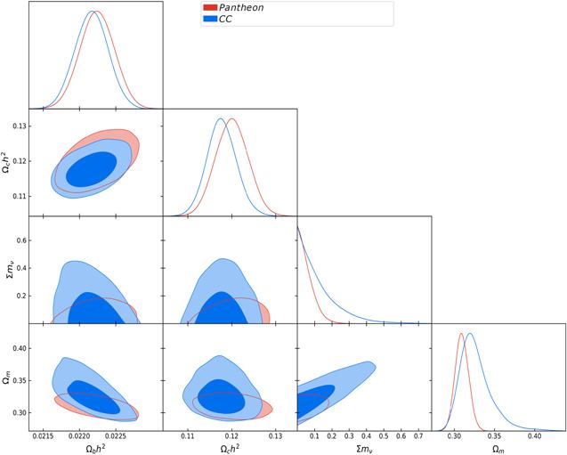
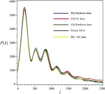
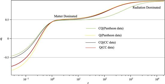
z). However, until recently, determining this redshift was possible was not acceptable because there were no high-quality data at sufficiently high redshifts (the redshift transition in standard dark energy cosmological models). In this paper, we first put constraints on the total mass of neutrinos and then estimate the Deceleration–Acceleration phase redshift transition using the coupling canonical scalar field with neutrinos. Then we investigate the effect of non-relativistic on the CMB power spectrum with the use of the CAMB code.

2. Quintessence model

In physics, quintessence is a hypothesized form of dark energy, more specifically a scalar field, that is hypothesized to explain the observed accelerated rate of expansion of the Universe. The first example of this scenario was proposed by [2123]. This concept was extended to more general types of time-varying dark energy, and the term ‘species of the essence’ was first coined in a 1998 paper by Robert R Caldwell, Rahul Dave, and Paul Steinhardt introduced [24]. It has been proposed by some physicists as the fifth fundamental force [2528]. It differs from the explanation of the cosmic constant of dark energy in dynamics. Quintessence can be attractive or repulsive, depending on the ratio of kinetic energy and its potential. We start with a scalar field minimally coupled to gravity. The action that represents our physical system is
$\begin{eqnarray}S=\int {{\rm{d}}}^{4}x\sqrt{-g}\left(\displaystyle \frac{R}{2{\kappa }^{2}}+{L}_{m}+{L}_{\phi }\right),\end{eqnarray}$
where Lφ is the Lagrangian of the scalar field as:
$\begin{eqnarray}{L}_{\phi }=\displaystyle \frac{-1}{2}{g}^{\mu \nu }{\partial }_{\mu }\phi {\partial }_{\nu }\phi -V(\phi ),\end{eqnarray}$
where V(φ) is a general self-coupling potential φ for which must be positive for physically acceptable fields. Differentiation with respect to gμν leads to the gravitational field equations
$\begin{eqnarray}{R}_{\mu \nu }=\displaystyle \frac{-1}{2}{g}_{\mu \nu }R=\kappa {T}_{\mu \nu }+{{T}_{\mu \nu }}^{(\phi )},\end{eqnarray}$
where
$\begin{eqnarray}{T}_{\mu \nu }^{(\phi )}={\partial }_{\mu }\phi {\partial }_{\nu }\phi -\displaystyle \frac{1}{2}{g}_{\mu \nu }{\left(\partial \phi \right)}^{2}-{g}_{\mu \nu }V(\phi ),\end{eqnarray}$
is the energy-momentum tensor of scalar field. By introduce:
$\begin{eqnarray}{\left(\partial \phi \right)}^{2}\equiv {g}_{\alpha \beta }{\partial }^{\alpha }\phi {\partial }^{\beta }\phi ,\end{eqnarray}$
which will be used later. Differentiation with respect to φ it shows the relation to the Klein–Gordon equation
$\begin{eqnarray}{{\rm{\nabla }}}_{\mu }{{\rm{\nabla }}}^{\mu }\phi -{V}_{,\phi }=0,\end{eqnarray}$
where ${V}_{,\phi }=\tfrac{\partial V}{\partial \phi }$. We consider a homogeneous and isotropic and completely flat universe and using the FLRW metric we have:
$\begin{eqnarray}{\mathrm{ds}}^{2}=-{\mathrm{dt}}^{2}+{{\rm{a}}}^{2}({\rm{t}})({\mathrm{dx}}^{2}+{\mathrm{dy}}^{2}+{\mathrm{dz}}^{2}).\end{eqnarray}$
In addition, the equation of state P = ωρ for the matter field is considered. With these assumptions, Einstein's field equations (3) are reduced to the following Friedman equations and acceleration:
$\begin{eqnarray}3{H}^{2}={\kappa }^{2}\left(\rho +\displaystyle \frac{1}{2}{\dot{\phi }}^{2}+V\right),\end{eqnarray}$
$\begin{eqnarray}2\dot{H}+3{H}^{2}=-{\kappa }^{2}\left(\omega \rho +\displaystyle \frac{1}{2}{\dot{\phi }}^{2}+V\right),\end{eqnarray}$
while the Klein–Gordon equation (6) is simplified as follows:
$\begin{eqnarray}(\ddot{\phi }+3H{\dot{\phi }}^{2}+{V}_{,\phi })=0.\end{eqnarray}$
The energy density and pressure of the scalar field are defined as follows:
$\begin{eqnarray}{\rho }_{\phi }=\displaystyle \frac{1}{2}{\dot{\phi }}^{2}+V,\end{eqnarray}$
$\begin{eqnarray}{P}_{\phi }=\displaystyle \frac{1}{2}{\dot{\phi }}^{2}-V.\end{eqnarray}$
Therefore, the equation of state is
$\begin{eqnarray}{\omega }_{\phi }=\displaystyle \frac{{P}_{\phi }}{{\rho }_{\phi }}=\displaystyle \frac{\tfrac{1}{2}{\dot{\phi }}^{2}-V}{\tfrac{1}{2}{\dot{\phi }}^{2}+V}.\end{eqnarray}$
Note that ωφ is a dynamically evolving parameter that can take values in the range [–1, 1].

3. Solving equations using dynamic system

The complete set of equations describing general linear perturbations for the model was shown in the previous section. These equations are a nonlinear set of second-order differential equations, with a large number of variables that have no analytical solution and can only be formulated in terms of numerical analysis. Our goal is to convert the second-order differential equation to the first-order by introducing several new variables. Since we are concerned with the possible applications of dynamical systems for such models, we must first solve the cosmological equations (8)–(10) in rewriting an independent system of equations. In general, there are many ways to achieve this, but the most common is to introduce EN variables:
$\begin{eqnarray}\zeta =\displaystyle \frac{\kappa \dot{\phi }}{\sqrt{6}H},\quad \eta =\displaystyle \frac{\kappa \sqrt{V}}{\sqrt{3}H}.\end{eqnarray}$
For a scalar field in the presence of baryonic matter, they were first introduced in a paper by Copeland et al (1998). Note that in the above definition, it is assumed that we are dealing with a positive definite scalar field potential. The evolution equations can be written as a phase plane-independent system:
$\begin{eqnarray}\displaystyle \frac{{\rm{d}}\zeta }{{\rm{d}}N}=-3\zeta +\sqrt{\displaystyle \frac{3}{2}}{\eta }^{2}+\zeta \displaystyle \frac{\dot{H}}{{H}^{2}},\end{eqnarray}$
$\begin{eqnarray}\displaystyle \frac{{\rm{d}}\eta }{{\rm{d}}N}=-\lambda \sqrt{\displaystyle \frac{3}{2}}\eta \zeta +\displaystyle \frac{3}{2}\eta +\zeta \displaystyle \frac{\dot{H}}{{H}^{2}},\end{eqnarray}$
where in N = lna. Also, the important parameter $\tfrac{\dot{H}}{{H}^{2}}$ in terms of new variables
$\begin{eqnarray}\displaystyle \frac{\dot{H}}{{H}^{2}}=-\displaystyle \frac{3}{2}(2{\eta }^{2}+\gamma (1-{\eta }^{2}-{\zeta }^{2})).\end{eqnarray}$
The above parameter is very useful for the connection between the theoretical model and observations. Using the above relation, we obtain the deceleration parameter, q, as well as the relation $q=-1-\tfrac{\dot{H}}{{H}^{2}}$, we arrive at the equation of the effective state: ${\omega }_{{eff}}=-\tfrac{1}{3}+\tfrac{2}{3}q$.

3.1. Coupling canonical scalar field with neutrinos

In this section, by considering mass neutrinos and adding the energy density and pressure of neutrinos to equations (8) and (9) and solving the equations in a previous way, we will investigate the Deceleration–Acceleration phase redshift transition zda. Einstein's field equations (3) are reduced to the following Friedman equations and acceleration :
$\begin{eqnarray}3{H}^{2}={\kappa }^{2}\left({\rho }_{m}+\displaystyle \frac{1}{2}{\dot{\phi }}^{2}+V(\phi )\right)+{\kappa }^{2}{\rho }_{\nu },\end{eqnarray}$
$\begin{eqnarray}2\dot{H}+3{H}^{2}=-{\kappa }^{2}\left(\omega {\rho }_{m}+\displaystyle \frac{1}{2}{\dot{\phi }}^{2}-V(\phi )\right)+{\kappa }^{2}{\omega }_{\nu }{\rho }_{\nu }.\end{eqnarray}$
The evolution equations for their energy densities are:
$\begin{eqnarray}{\dot{\rho }}_{\phi }+3H{\rho }_{\phi }(1+{\omega }_{\phi })=-\beta {\rho }_{\nu }(1-3{\omega }_{\nu })\dot{\phi },\end{eqnarray}$
$\begin{eqnarray}{\dot{\rho }}_{\nu }+3H{\rho }_{\nu }(1+{\omega }_{\nu })=\beta {\rho }_{\nu }(1-3{\omega }_{\nu })\dot{\phi },\end{eqnarray}$
where the β is the coupling constant and ρν is the energy density of neutrinos. The Klein–Gordon equation is:
$\begin{eqnarray}\begin{array}{rcl}\ddot{\phi } & = & \lambda V(\phi )-\displaystyle \frac{3}{2}H\dot{\phi }(1+{\omega }_{\phi })-\displaystyle \frac{3{HV}}{\dot{\phi }}(1+{\omega }_{\phi })\\ & & -\beta {\rho }_{\nu }(1-3{\omega }_{\nu }).\end{array}\end{eqnarray}$
We rewrite the cosmological equations (18)–(20) into an autonomous system of equations.
$\begin{eqnarray}{\chi }_{1}=\displaystyle \frac{{\kappa }^{2}{\rho }_{m}}{3{H}^{2}},\,{\chi }_{2}=\displaystyle \frac{\kappa \dot{\phi }}{\sqrt{6}H},\,{\chi }_{3}=\displaystyle \frac{{\kappa }^{2}V(\phi )}{3{H}^{2}},\,{\chi }_{4}=\displaystyle \frac{{\kappa }^{2}{\rho }_{\nu }}{3{H}^{2}}.\end{eqnarray}$
We can derive the following dynamical system:
$\begin{eqnarray}\displaystyle \frac{{\rm{d}}{\chi }_{1}}{{\rm{d}}N}=-3{\chi }_{1}-2{\chi }_{1}\displaystyle \frac{\dot{H}}{{H}^{2}},\end{eqnarray}$
$\begin{eqnarray}\begin{array}{rcl}\displaystyle \frac{{\rm{d}}{\chi }_{2}}{{\rm{d}}N} & = & \displaystyle \frac{3\lambda }{\sqrt{6}\kappa }{\chi }_{3}-\displaystyle \frac{3}{2}(1+{\omega }_{\phi }){\chi }_{2}-\displaystyle \frac{3}{2}(1+{\omega }_{\phi })\displaystyle \frac{{\chi }_{3}}{{\chi }_{2}}\\ & & -\displaystyle \frac{3\kappa \beta }{\sqrt{6}}(1-3{\omega }_{\nu }){\chi }_{4}-{\chi }_{2}\displaystyle \frac{\dot{H}}{{H}^{2}},\end{array}\end{eqnarray}$
$\begin{eqnarray}\begin{array}{rcl}\displaystyle \frac{{\rm{d}}{\chi }_{4}}{{\rm{d}}N} & = & -3(1+{\omega }_{\nu }){\chi }_{4}+\displaystyle \frac{\beta \sqrt{6}(1-3{\omega }_{\nu })}{\kappa }{\chi }_{2}{\chi }_{4}\\ & & -2{\chi }_{4}\displaystyle \frac{\dot{H}}{{H}^{2}}.\end{array}\end{eqnarray}$
The Friedmann constraint is
$\begin{eqnarray}{\chi }_{3}=1-{\chi }_{1}-{\chi }_{2}^{2}-{\chi }_{4}.\end{eqnarray}$
Also
$\begin{eqnarray}\displaystyle \frac{\dot{H}}{{H}^{2}}=\displaystyle \frac{3}{2}\left(-1-{\omega }_{m}{\chi }_{1}-{\chi }_{2}^{2}+{\chi }_{3}+{\omega }_{\nu }{\chi }_{4}\right).\end{eqnarray}$
Before discussing the effect of mass neutrinos on the phase transition redshift value, we first estimate the neutrino mass using the coupling of scalar field and neutrino. We used the same approach with [29] to put constraints on the total mass of neutrinos.

4. Estimate the neutrino mass

We have considered a cosmological model in which dark energy and neutrinos are coupled such that the mass of the neutrinos and potentials are functions of the scalar field as ${m}_{\nu }={m}_{0}{{\rm{e}}}^{\left(\tfrac{\beta \phi }{{m}_{{pl}}}\right)}$ and $V(\phi )={{m}_{{pl}}}^{4}{{\rm{e}}}^{\left(\tfrac{-\lambda \phi }{{m}_{{pl}}}\right)}$. In equation (23), χ1, χ4 are equivalent to Ωm and Ων. We calculate the Ων by solving the above equations and calculating the total mass of the neutrino $\left({{\rm{\Omega }}}_{\nu }=\tfrac{\sum {m}_{\nu }}{93.14{h}^{2}}\right)$. Where h is the reduced Hubble constant. Hence if the parameters (h, Ων ) are constrained then the parameter ∑mν is constrained automatically. The relativistic energy density in the early universe includes the contributions from photons and neutrinos, and possibly other extra relativistic degrees of freedom, called dark radiation. The standard value of Neff is 3.046 corresponding to the case with three-generation neutrinos and no extra dark radiation. Thus, the total radiation energy density in the Universe is given by
$\begin{eqnarray}{\rho }_{r}={\rho }_{\gamma }\left(1+\frac{7}{8}{\left(\frac{4}{11}\right)}^{\tfrac{4}{3}}{N}_{\mathrm{eff}}\right),\end{eqnarray}$
where ργ is the energy density of photons. The effective number of relativistic species of neutrinos(Neff) related to matter density, Ωmh2 and zeq (redshift of matter-radiation equality) through below equation
$\begin{eqnarray}{N}_{\mathrm{eff}}=3.04+7.44\left(\frac{{{\rm{\Omega }}}_{m}{h}^{2}}{0.1308}\frac{3139}{1+{z}_{\mathrm{eq}}}-1\right).\end{eqnarray}$
We use the pantheon catalog (1048 supernova type Ia) and c.c. (cosmic chronometers) data to put constraints on the (Ωm, λ, h, Ων ).
The results of best fitting parameter are shown in table 1.
Table 1. Observational constraints at 95% on main and derived parameters of the ∑mν scenario. The parameter H0 is in the units of km/sec/Mpc, whereas ∑mν reported in the 95% CL, is in the units of eV.
Model Ωbh2 Ωch2 H0 Ωm mν λ zda
Quintessense(Pantheon) ${0.0222}_{-0.0003}^{+0.0005}$ ${0.1181}_{-0.0001}^{+0.00012}$ ${69.8}_{-0.2}^{+0.1}$ ${0.305}_{-0.002}^{+0.002}$ <0.19 ${0.2}_{-0.03}^{+0.01}$ 0.42 ± 0.03
Quintessense(CC) ${0.0224}_{-0.00012}^{+0.00012}$ ${0.1169}_{-0.00018}^{+0.00018}$ ${69.7}_{-0.5}^{+0.5}$ ${0.302}_{-0.02}^{+0.02}$ <0.39 ${0.8}_{-0.09}^{+0.09}$ 0.49 ± 0.05
ΛCDM ${0.022}_{-0.00049}^{+0.00053}$ ${0.122}_{-0.000312}^{+0.000325}$ ${67.5}_{-2.0}^{+2.0}$ ${0.301}_{-0.015}^{+0.015}$ <0.12

5. Linear perturbations

For analyzing perturbations in scalar elds and matter we work in the longitudinal gauge [3133]. For scalar eld and for pressure less matter (described as perfect uid). We start from a system-perturbed FRW metric as follows
$\begin{eqnarray}{\mathrm{ds}}^{2}=(1+2{\rm{\Phi }}){\mathrm{dt}}^{2}-{{\rm{a}}}^{2}({\rm{t}})(1-2{\rm{\Phi }})[{\mathrm{dx}}^{2}+{\mathrm{dy}}^{2}+{\mathrm{dz}}^{2}].\end{eqnarray}$
The energy momentum tensor of a perfect uid is described as:
$\begin{eqnarray}{T}_{\nu }^{\mu }=(\rho +p){u}^{\mu }{u}_{\nu }-p{\delta }_{\nu }^{\mu }.\end{eqnarray}$
Perturbations in the energy density ρ, pressure p and the four velocity uμ are defined as:
$\begin{eqnarray}\rho (t,\vec{x})={\rho }_{0}(t)+\delta \rho (t,\vec{x}),\end{eqnarray}$
$\begin{eqnarray}p(t,\vec{x})={p}_{0}(t)+\delta p(t,\vec{x}),\end{eqnarray}$
$\begin{eqnarray}{u}^{\mu }={{u}^{0}}^{\mu }+\delta {u}^{\mu },\end{eqnarray}$
where ${{u}^{0}}^{\mu }=\{1,0,0,0\};$ ρ0(t) and p0(t) are average values of the energy density and pressure respectively on a constant time hyper surface. For scalar (quintessence) eld with Lagrangian of the form equation (2), we define the perturbations as:
$\begin{eqnarray}\phi (\tilde{{\rm{x}}},\ {\rm{t}})={\phi }_{0}({\rm{t}})+\delta \phi (\tilde{{\rm{x}}},{\rm{t}}),\end{eqnarray}$
where φ0(t) is the average value of the scalar eld on the constant time hyper surface. The energy momentum tensor for the scaler eld is given by
$\begin{eqnarray}{T}_{\nu }^{\mu }={\partial }^{\mu }\phi {\partial }_{\nu }\phi -{L}_{\phi }{\delta }_{\nu }^{\mu }.\end{eqnarray}$
Substituting equations (37) in (38) and subtracting the homogeneous part in the energy momentum tensor we get
$\begin{eqnarray}\begin{array}{l}\delta {T}_{0}^{0}=\delta {\rho }_{\phi }={\dot{\phi }}_{0}\dot{\delta }\phi -{\rm{\Phi }}{{\dot{\phi }}_{0}}^{2}+V^{\prime} ({\phi }_{0})\delta \phi ,\\ \delta {T}_{j}^{i}=-\delta {p}_{\phi }{\delta }_{j}^{i}=-[{\dot{\phi }}_{0}\dot{\delta }\phi -{\rm{\Phi }}{{\dot{\phi }}_{0}}^{2}-V^{\prime} ({\phi }_{0})\delta \phi ]{\delta }_{j}^{i},\\ \delta {T}_{0}^{i}=({\rho }_{\phi 0}+{p}_{\phi 0})\delta {u}_{i(\phi )}={\dot{\phi }}_{0}\delta {\phi }_{,i}.\end{array}\end{eqnarray}$
The perturbed Einstein's equation about a at FRW metric is given by $\delta {G}_{\nu }^{\mu }=8\pi G\delta {T}_{\nu }^{\mu }$. In our case $\delta {T}_{\nu }^{\mu }=\delta {T}_{\nu (\mathrm{matter})}^{\mu }\,+\delta {T}_{\nu (\phi )}^{\mu }$. Since the matter has negligible pressure we set $\delta {T}_{\nu (\mathrm{matter})}^{\mu }=0$. Fluctuation in pressure is contributed only by the scalar eld. With attention to the above equations, we obtain the following linearized Einstein's equations :
$\begin{eqnarray}3{H}^{2}{\rm{\Phi }}+3H\dot{{\rm{\Phi }}}+\displaystyle \frac{{K}^{2}{\rm{\Phi }}}{{a}^{2}}=-4\pi G[\delta {\rho }_{m}+{\dot{\phi }}_{0}\dot{\delta }\phi -{\rm{\Phi }}{{\dot{\phi }}_{0}}^{2}+V^{\prime} ({\phi }_{0})\delta \phi ],\end{eqnarray}$
$\begin{eqnarray}\ddot{{\rm{\Phi }}}+4H\dot{{\rm{\Phi }}}+2\dot{H}{\rm{\Phi }}-{H}^{2}{\rm{\Phi }}=4\pi G[{\dot{\phi }}_{0}\dot{\delta }\phi -{\rm{\Phi }}{{\dot{\phi }}_{0}}^{2}-V^{\prime} ({\phi }_{0})\delta \phi ],\end{eqnarray}$
$\begin{eqnarray}\dot{{\rm{\Phi }}}+H{\rm{\Phi }}=4\pi G({\rho }_{0}{a}^{-3}{v}_{m}+{\dot{\phi }}_{0}\delta \phi ),\end{eqnarray}$
where $V^{\prime} ({\phi }_{0})=\tfrac{\partial V({\phi }_{0})}{\partial {\phi }_{0}}$ and vm is the potential for the matter peculiar velocity. The perturbed quantities are Φ, δφ, δρm and vm. Where K is the wave number defined as $K=\tfrac{2\pi }{{\lambda }_{p}}$ and λp is the comoving length scale of perturbation. In addition to this, the dynamical equation for the perturbations in the scalar eld δφ(t) is obtained from the scalar eld Lagrangian (2) and this is given by :
$\begin{eqnarray}\ddot{\delta }\phi +3H\dot{\delta }\phi +\displaystyle \frac{{K}^{2}\delta \phi }{{a}^{2}}+2{\rm{\Phi }}V^{\prime} ({\phi }_{0})-4\dot{{\rm{\Phi }}}{{\dot{\phi }}_{0}}^{2}+V^{\prime\prime} ({\phi }_{0})\delta \phi =0.\end{eqnarray}$
For solving the background equations [equations (40) and (41)], we introduce the following dimensionless variables:
$\begin{eqnarray}\begin{array}{l}{\xi }_{1}=\displaystyle \frac{-\delta {\rho }_{m}}{6{H}^{2}{\rm{\Phi }}},\quad {\xi }_{2}=\displaystyle \frac{-{\dot{\phi }}_{0}\dot{\delta }\phi }{6{H}^{2}{\rm{\Phi }}},\\ {\xi }_{3}=\displaystyle \frac{{{\dot{\phi }}_{0}}^{2}}{6{H}^{2}},\quad {\xi }_{4}=\displaystyle \frac{-V^{\prime} ({\phi }_{0})\delta \phi }{6{H}^{2}{\rm{\Phi }}},\\ {\xi }_{5}=\displaystyle \frac{-\dot{{\rm{\Phi }}}}{H{\rm{\Phi }}},\quad {\xi }_{6}=\displaystyle \frac{-{K}^{2}}{3{H}^{2}{a}^{2}}.\end{array}\end{eqnarray}$
We can derive the following dynamical system:
$\begin{eqnarray}\begin{array}{rcl}\displaystyle \frac{{\rm{d}}{\xi }_{2}}{{\rm{d}}N} & = & -{\xi }_{2}-{\xi }_{4}{{\rm{\Gamma }}}_{1}-\displaystyle \frac{{\xi }_{6}}{2}{{\rm{\Gamma }}}_{3}-2{\xi }_{4}{{\rm{\Gamma }}}_{3}\\ & & +4{\xi }_{5}{\xi }_{6}-2{\xi }_{2}\displaystyle \frac{\dot{H}}{{H}^{2}}+\lambda {\xi }_{4}\sqrt{6{\xi }_{3}},\\ \displaystyle \frac{{\rm{d}}{\xi }_{3}}{{\rm{d}}N} & = & 6{\xi }_{2}{\psi }_{2}+2{\xi }_{4}{{\rm{\Gamma }}}_{1}{\psi }_{2}\sqrt{6{\xi }_{3}}-{\xi }_{3}\displaystyle \frac{\dot{H}}{{H}^{2}},\\ \displaystyle \frac{{\rm{d}}{\xi }_{4}}{{\rm{d}}N} & = & {\xi }_{4}\sqrt{6{\xi }_{3}}+{\xi }_{4}{{\rm{\Gamma }}}_{1}+{\xi }_{4}{\xi }_{5}+2{\xi }_{4}\displaystyle \frac{\dot{H}}{{H}^{2}},\\ \displaystyle \frac{{\rm{d}}{\xi }_{5}}{{\rm{d}}N} & = & 3{\xi }_{2}+{\xi }_{3}-3{\xi }_{4}-4{\xi }_{5}-\displaystyle \frac{\dot{H}}{{H}^{2}}(1+{\xi }_{5})+{{\xi }_{5}}^{2},\\ \displaystyle \frac{{\rm{d}}{\xi }_{6}}{{\rm{d}}N} & = & -2{\xi }_{6}-2{\xi }_{6}\displaystyle \frac{\dot{H}}{{H}^{2}},\end{array}\end{eqnarray}$
with
$\begin{eqnarray}\begin{array}{rcl}\displaystyle \frac{\dot{H}}{{H}^{2}} & = & 3({\xi }_{2}+{\xi }_{3}-{\xi }_{4})-4{\xi }_{4}-1-4.5{\xi }_{6}{\psi }_{4}\\ & & -1.5{\psi }_{1}\sqrt{6{\xi }_{3}}+3({\xi }_{2}+{\xi }_{4})+{\xi }_{5},\end{array}\end{eqnarray}$
and we use the fiedmann constraint
$\begin{eqnarray}{\xi }_{1}=-1+{\xi }_{2}-{\xi }_{3}+{\xi }_{4}+{\xi }_{5}+{\xi }_{6}.\end{eqnarray}$
In above equations we introduce new variables
$\begin{eqnarray}{{\rm{\Gamma }}}_{1}=\displaystyle \frac{\dot{\delta }\phi }{H\delta \phi },\quad {{\rm{\Gamma }}}_{2}=\displaystyle \frac{{\dot{\phi }}_{0}\delta \phi }{H},\quad {{\rm{\Gamma }}}_{3}=\displaystyle \frac{{\dot{\phi }}_{0}}{H\delta \phi },\end{eqnarray}$
$\begin{eqnarray}{\psi }_{1}=\displaystyle \frac{\delta \phi }{{\rm{\Phi }}},\,\,{\psi }_{2}={\rm{\Phi }},\,\,{\psi }_{3}=\displaystyle \frac{{\rho }_{0}{v}_{m}}{{a}^{3}H},\,\,{\psi }_{4}=\displaystyle \frac{{\rho }_{0}{v}_{m}}{{aK}}.\end{eqnarray}$
By using the same approach
$\begin{eqnarray}\begin{array}{rcl}\displaystyle \frac{{\rm{d}}{{\rm{\Gamma }}}_{1}}{{\rm{d}}N} & = & -3{{\rm{\Gamma }}}_{1}+{\xi }_{6}+12{\xi }_{4}{\psi }_{1}+4{\xi }_{5}{{\rm{\Gamma }}}_{3}+\lambda {\xi }_{4}{\psi }_{1},\\ \displaystyle \frac{{\rm{d}}{{\rm{\Gamma }}}_{2}}{{\rm{d}}N} & = & -6{\xi }_{2}\displaystyle \frac{{\psi }_{2}}{{{\rm{\Gamma }}}_{1}},\\ \displaystyle \frac{{\rm{d}}{{\rm{\Gamma }}}_{3}}{{\rm{d}}N} & = & -3{{\rm{\Gamma }}}_{3}+6{\xi }_{2}{\psi }_{2}+\sqrt{6{\xi }_{3}}\displaystyle \frac{\dot{H}}{{H}^{2}}+\sqrt{6{\xi }_{3}}{{\rm{\Gamma }}}_{1},\end{array}\end{eqnarray}$
and
$\begin{eqnarray}\begin{array}{rcl}\displaystyle \frac{{\rm{d}}{\psi }_{1}}{{\rm{d}}N} & = & {\psi }_{1}({{\rm{\Gamma }}}_{1}+{\xi }_{5}),\\ \displaystyle \frac{{\rm{d}}{\psi }_{2}}{{\rm{d}}N} & = & {\psi }_{3}+\displaystyle \frac{{{\rm{\Gamma }}}_{3}}{2}+{\psi }_{2},\\ \displaystyle \frac{{\rm{d}}{\psi }_{3}}{{\rm{d}}N} & = & -6K{\psi }_{3}-{\psi }_{3}\displaystyle \frac{\dot{H}}{{H}^{2}},\\ \displaystyle \frac{{\rm{d}}{\psi }_{4}}{{\rm{d}}N} & = & -{\psi }_{4}.\end{array}\end{eqnarray}$

5.1. Cosmic evolution in presence of non-relativistic neutrino

The neutrinos of the early universe evolved from a relativistic phase at very early times to a massive particle behavior at later times. First, the kinetic energy of neutrinos is relativistic, and as a result, neutrinos can be described as massless particles. As the Universe expands, the temperature drops and the kinetic energy decreases, and the neutrinos turn into a non-relativistic phase with a non-negligible mass. This means that neutrinos contribute to radiation at early times and to matter after the transition, with an energy density given by
$\begin{eqnarray}{\rho }_{\nu }({m}_{\nu }\ll {T}_{\nu })=\frac{7{\pi }^{2}}{120}{\left(\frac{4}{11}\right)}^{\tfrac{4}{3}}{N}_{\mathrm{eff}}{T}_{\gamma }^{4}=\frac{7}{8}{\left(\frac{4}{11}\right)}^{\tfrac{4}{3}}{N}_{\mathrm{eff}}{\rho }_{\gamma },\end{eqnarray}$
$\begin{eqnarray}{\rho }_{\nu }({m}_{\nu }\gg {T}_{\nu })=\displaystyle \frac{{\rho }_{c}}{93.14{h}^{2}{ev}}\displaystyle \sum _{\,}{m}_{\nu },\end{eqnarray}$
where Tν and Tγ are the neutrino and photon temperatures respectively, ργ is the photon density, and h is the dimensionless Hubble constant. The two parameters of this model are the effective number of relativistic species, Neff, and the total neutrino mass, ${\sum }_{}^{}{m}_{\nu }$.
When neutrinos become non-relativistic, they play a more important role in cosmic evolution. Primary CMB anisotropies are only mildly affected, but the interaction of CMB photons with the low-redshift universe and the formation and growth of large-scale structures will have strong signatures of the neutrino mass. Neutrinos do not cluster like a normal matter component. By explicitly comparing the expression of the matter power spectrum, P(k), for massless and massive neutrinos, the power spectrum is suppressed as [30]
$\begin{eqnarray}\displaystyle \frac{p(k,\displaystyle \sum _{}{m}_{\nu })-p(k,\displaystyle \sum _{}{m}_{\nu }=0)}{p(k,\displaystyle \sum _{}{m}_{\nu }=0)}\approx -0.08\left(\displaystyle \frac{\sum {m}_{\nu }}{1{ev}}\right)\displaystyle \frac{1}{{{\rm{\Omega }}}_{m}{h}^{2}},\end{eqnarray}$
where the Ωm is the matter density.

6. Numerical analysis

In this paper, we use the Pantheon dataset (Steinhardt et al 2020) of 1048 supernovae covering the redshift 0.015 < z < 2.3 range and CC data covering the redshift 0.07 < z < 2.5 and used Markov Chain Monte Carlo (MCMC) approach. In the MCMC method, which was coded in MATLAB software, the node method was used, which is the most famous and accurate method in solving partial differential equations with the help of Monte Carlo. We will also discretize all the equations and solve them using the random function method that generates random data and we will reach the solution with high accuracy. The advantages of the Monte Carlo method are that the code volume is reduced in this method. With fewer loops, the answer was obtained with a higher speed and less time. In this method, it is easier to add equations and enlarge the system of equations. In the following, we investigate the effect of neutrinos on the matter power spectrum, P(k), in the case of massless and massive neutrinos using the publicly available Boltzmann code CAMB and we prove that when neutrino coupled to scalar field the CMB power spectrum have a little shift which means that the power spectrum of CMB is greatly affected by the background energy density and the accelerated expansion of the Universe.
For an explanation of figure 2:

The first peak corresponding to the horizontal sound, which is the distance of the sound wave, extends until the coupling time. This mode is the longest wavelength of the fluctuations of sound waves. Fluctuations in this scale are prominent fluctuations that were present in the last scattering in the plasma. In addition, this mode reaches a maximum fluctuation at the time of coupling. Therefore, the first peak is also the highest peak in the power spectrum.

Second peak: the amplitude of the second peak is related to the baryon density in the Universe.

Higher peaks: the amplitude of the third peak can be used to determine the dark matter density.

Damping tail: the damping tail of the CMB temperature anisotropy power spectrum depends on the photon diffusion length at recombination.

The amount of baryonic matter affects the height of each peak. If the baryonic matter increases, the value of the individual peaks corresponding to the plasma pressure becomes higher. The even peaks corresponding to plasma dilution will be shorter. So for more baryons, we have longer odd peaks and shorter even peaks.
As we see in figure 2, because the Ωbh2 value obtained for analyses of CC data is greater than the value of the Pantheon data, the first peak of the CMB power spectrum of CC data analyses is higher than Pantheon data. These results indicate that when the mass of neutrinos increases, the value of the background energy density increases and resulting in a higher power spectrum peak. In the previous part, the relation of the deceleration parameter was mentioned, now by examining the deceleration parameter in different periods of cosmology, its evolution was investigated. In the continuation of this article and using the above equations, we examine the deceleration parameter for the coupled quintessence model with neutrino and the uncoupled model with two Pantheon and CC data, and the results are shown in figure 3. By using the above equations and the Monte Carlo method and reconstruction of the deceleration parameter (q), the Deceleration–Acceleration redshift transition zda = 0.7 ± 0.05 value was obtained for pantheon data and zda = 0.68 ± 0.03 for CC data which is close to result in obtained in [15]. In presence of neutrinos the DA redshift transition is zda = 0.42 ± 0.03 for Pantheon data and zda = 0.49 ± 0.05 for CC data which is in good agreement with the [16] results. Figure 1 shows the results of our analysis and in figures 2 and 3, we plot the 95% CL two-dimensional contours for ∑mν for both Pantheon and CC data. Also, in tables 2, 3 a comparison of the results of our analysis with the work of other scientists is shown. In table 3 we Compare Ωbh2, Ωch2, H0, Ωm obtained values in Quintessence model in presence of neutrino in CC and Pantheon data.
Figure 1. Comparison of Ωbh2 , Ωch2 , H0 , Ωm obtained values in Quintessence model.
Figure 2. Comparison the CMB power spectrum of Planck 2018 result and coupled quintessence and Perturbed quintessence(PQ).
Figure 3. Comparison of the zda between quintessence and coupled quintessence models for CC and Pantheon data.(CQ is coupled quintessence and Q is quintessencs model).
Table 2. Comparison between both zda and ∑mν for quintessence model without neutrino and quintessence model in presence of neutrino (for pantheon data).
Σmν(ev) zda Approach Reffrence
0.71 ± 0.05 Without Neutrino [15]
<0.19 0.42 ± 0.03 With Neutrino [16]
Table 3. Comparison between both zda and ∑mν for quintessence model without neutrino and quintessence model in presence of neutrino (for c.c. data).
Σmν(ev) zda Approach Reffrence
0.68 ± 0.03 Without Neutrino [15]
<0.38 0.49 ± 0.05 With Neutrino [16]
Furthermore, we consider the effect of perturbed quintessence (PQ) on the CMB power spectrum and find that: the locations and the heights of the CMB anisotropy peaks have been changed due to the coupling and perturbation of the quintessence scalar field. Especially, there is a significant difference in the heights of the second and the third peaks among the models. for l ≥ 200 we can see that the locations of the acoustic peaks are slightly shifted to smaller scales. The third peak in this model is smaller than that in the ΛCDM model. These results are shown in figure 2.

7. Conclusion

The cosmic microwave background waves are the remnants of the big bang at the beginning of the cosmological era. These waves are proof of the existence of this explosion and the theories based on it, such as the standard model and the inflation model, and it has a temperature distribution that is relatively uniform but has temperature anisotropies. These anisotropies are the result of density disturbances that happened during the big explosion. In this paper, we first put constraints on the total mass of neutrinos and then estimate the Deceleration–Acceleration redshift transition using the coupling canonical scalar field with neutrinos. For Pantheon data, we obtained zda = 0.7 ± 0.05 and for CC data zda = 0.68 ± 0.03 which consists of the result obtained in [15]. In presence of neutrinos the DA redshift transition is zda = 0.42 ± 0.03 for Pantheon data and zda = 0.49 ± 0.05 for CC data which is in good agreement with the [16] results, which indicate that neutrinos can affect this phase transition. Also, we investigate the effect of neutrinos on the matter power spectrum, P(k), in the case of massless and massive neutrinos and we prove that when neutrinos are coupled to a scalar field the matter power spectrum has a little shift which means that when neutrinos are coupled to a scalar field the CMB power spectrum has a little shift which means that the power spectrum of CMB is greatly affected by the background energy density and the accelerated expansion of the Universe. The results obtained in this article show that when the mass of neutrinos increases, the value of the background energy density increases and resulting in a higher power spectrum peak. Also, by examining the effect of coupling of neutrinos to dark energy, we obtained that the transition occurs at lower redshift.
Also, we consider the effect of perturbed quintessence (PQ) on the CMB power spectrum and find that: the locations and the heights of the CMB anisotropy peaks have been changed due to the coupling and perturbation of the quintessence scalar field. Especially, there is a significant difference in the heights of the second and the third peaks among the models. for l ≥ 200 we can see that the locations of the acoustic peaks are slightly shifted to smaller scales. The third peak in this model is smaller than that in the ΛCDM model. These results are shown in figure 2.

Acknowledgments

I am incredibly grateful to the dear reviewer for the significant and valuable comments which caused this manuscript to improve considerably.
1
Amendola L Baldi M Wetterich Ch 2008 Growing matter Phys. Rev. D 78 023015

DOI

2
Nunes N J Schrempp L Wetterich C 2011 Mass freezing in growing neutrino quintessence Phys. Rev. D 83 083523

DOI

3
Wetterich C 2007 Growing neutrinos and cosmological selection Phys. Lett. B 655 201 208

DOI

4
Casas S Pettorino V Wetterich C 2016 Dynamics of neutrino lumps in growing neutrino quintessence Phys. Rev. D 94 103518

DOI

Mohseni Sadjadi S H Anari V 2018 Cosmic acceleration and de Sitter expansion in hybrid mass varying neutrino model J. Cosmol. Astropart. Phys. 10 036

DOI

5
Mohseni Sadjadi H Anari V 2020 End of the constant-roll inflation, and the reheating temperature Phys. Dark Universe 27 100474

DOI

6
Anari V Mohseni Sadjadi H 2022 End of the constant-roll inflation, and the reheating temperature J. Cosmol. Astropart. Phys. 07 043

DOI

7
Mohseni Sadjadi H Anari V 2017 Mass varying neutrinos, symmetry breaking, and cosmic acceleration Phys. Rev. D 95 123521

DOI

8
Spergel D N Pen U-L 1996 Cosmology in a string-dominated universe ApJ 491 L67

DOI

9
Banks T 1996 SUSY breaking, cosmology, vacuum selection and the cosmological constant in string theory arXiv:hep-th/9601151

10
Kepuladze Z Maziashvili M 2021 A new take on the inflationary quintessence Phys. Rev. D 103 063540

DOI

11
Steinhardt P J Wang L Zlatev I 1999 Cosmological tracking solutions Phys. Rev. 59 123504 D

DOI

12
Ratra B Peebles P J E 1988 Cosmological consequences of a rolling homogeneous scalar field Phys. Rev. D 37 3406

DOI

13
Peebles P J E Ratra B 1988 Cosmology with a time-variable cosmological ‘constant’ ApJ 325 L17

DOI

14
Binetruy P 1999 Models of dynamical super symmetry breaking and quintessence Phys. Rev. D 60 063502

DOI

15
Farooq O 2013 Hubble parameter measurement constraints on the cosmological deceleration–acceleration transition redshift Astrophys. J. 766 L7

DOI

16
Vargas dos Santos M Reis R R R 2016 Constraining the cosmic deceleration-acceleration transition with type Ia supernova, BAO/CMB and H(z) data Ioav Waga Astrophys. J. 02 066

DOI

17
Ishida E E Reis R R Toribio A V Waga I 2007 When did cosmic acceleration start? How fast was the transition? Astropart. Phys. 28 547 552

DOI

18
Turner M S Riess A G 2002 Do type Ia supernovae provide direct evidence for past deceleration of the universe? Astrophys. J. 569 18

DOI

19
Giostri R 2012 From cosmic deceleration to acceleration: new constraints from SN Ia and BAO/CMB J. Cosmol. Astropart. Phys. 2012 027

DOI

20
Farooq O 2017 Hubble parameter measurement constraints on the redshift of the deceleration–acceleration transition, dynamical dark energy, and space curvature Astrophys. J. 835 26

DOI

21
Ratra B Peebles L P 1988 Cosmological consequences of a rolling homogeneous scalar field Phys. Rev. D 37 3406

DOI

22
Wetterich C 1988 Cosmology and the fate of dilatation symmetry Nucl. Phys. B 302 668 696

23
Doran M 2001 Quintessence and the separation of cosmic microwave background peaks Astrophys. J. 559 501

DOI

24
Caldwell R R Dave R Steinhardt P J 1998 Cosmological imprint of an energy component with general equation of state Phys. Rev. Lett. 80 1582

DOI

25
Carroll S M 1998 Quintessence and the rest of the world: suppressing long-range interactions Phys. Rev. Lett. 81 3067

DOI

26
Wetterich, C Heidelberg University

27
Dvali G Zaldarriaga M 2002 Changing alpha with time: implications for fifth-force-type experiments and quintessence

28
Cicoli M Pedro F G Tasinato G 2012 Natural quintessence in string theory

29
Amiri H R Salehi A Noroozi A H 2021 Constraining neutrino mass in dark energy dark matter interaction and comparison with 2018 Planck results Eur. Phys. J. 81 479 C

DOI

30
Hu W Eisenstein D J Tegmark M 1998 Weighing neutrinos with galaxy surveys Phys. Rev. Lett. 80 5255 5258

DOI

31
Bardeen J 1980 Gauge-invariant cosmological perturbations Phys. Rev. D 22 1882

DOI

32
Kodama H Sasaki M 1984 Cosmological perturbation  theory Prog. Theor. Phys. Suppl. 78 1

DOI

33
Mukhanov V F Feldman H A Branden-berger R H 1992 Theory of cosmological perturbations Phys. Rep. 215 203

DOI

Outlines

/