


1. Introduction
Polariton condensates realized in semiconductor microcavities have recently become a competitive alternative to atomic Bose–Einstein condensates (BECs), due to their high condensation temperature, strong light–matter interactions and non-equilibrium properties [1–9]. These characteristics make such condensates an ideal platform for studying the exotic properties of quantum and non-equilibrium physics. The strong interaction induces rich nonlinear phenomena, such as bistability [10, 11], information processing [12–14], pattern formation [15–18], quantum vortices [19–25], space solitons [22, 23, 26–37] and so on.
As a fundamental type of nonlinear wave, shock waves, which are called dissipative shock waves or viscous shock waves in dissipative fluids and dispersive shock waves in dispersive fluids, appear in plasmas [38], fluids (e.g. undular bores) [39, 40], superfluids [41–44] and optics [45–48]. Generally, shock waves have the characteristics of multi-scale, unstable and rank-ordered oscillatory wave structures. At present, research on shock waves in integrable systems is relatively mature, and the solution structures can be obtained by using the weak dispersion approximation and discussion of the Riemann problem [49, 50], following which the shock waves and their asymptotic behaviors can be further analyzed [51–54]. However, it is difficult to discuss shock waves in non-integrable systems, especially in non-equilibrium systems.
In a polariton condensation system, the first report on shock waves was experimental [55, 56]; however, resonantly coherent pumping was used so that it was not certain whether the coherence of the condensation system originated from the BEC or laser. So, incoherent pumped polariton condensation became the focus of theoretical and experimental research. There are two theoretical reports on shock waves [57, 58], in which the approximation model neglecting the dispersion term and the interaction between polariton condensation and the reservoir and an approximation perturbation method are respectively adopted. These approximations result in only one kind of shock wave and one or two adjustable parameters (the coefficients of the non-equilibrium term). However, in incoherent polariton condensation, there are many controllable parameters, making it possible to generate various shock waves and control them.
In this paper, we introduce a coupled model with eight parameters to depict the evolution of incoherent pumped polariton condensates. Then, various shock waves are found by the initial input of step waves, and in different parameter spaces, the regions of existence of various shock waves are shown. We also discuss the effect of the amplitude and phase of the initial input wave, the self-interaction (Kerr nonlinearity) of condensates, the cross-interaction (saturated nonlinearity) between condensation and reservoir, the intensity of pumping, the condensation rate from polariton to condensate, and the spatial diffusion rate of the reservoir density on the region of existence of shock waves. In addition, we extend the range of existence of shock waves not only from the weak dispersion system to the normal dispersion system but also from Kerr nonlinearity to mixed nonlinearity, consisting of saturation and Kerr nonlinearities. Our proposal opens the way to generate and control shock waves in an incoherent pumped polariton condensation system.
2. Model
Under the framework of mean-field theory, we consider a polariton condensation setting trapped in a one-dimensional nanowire system. The generalized drive-dissipation Gross–Pitaevskii equation for the wave function $\Psi$(x, t) of polariton condensates coupled to the rate equation for the reservoir density nR(x, t) of the polariton is
$\begin{eqnarray}\begin{array}{l}{\rm{i}}{\hslash }\displaystyle \frac{\partial {\rm{\Psi }}}{\partial t}=\left[-\displaystyle \frac{{{\hslash }}^{2}}{2{m}^{* }}\displaystyle \frac{{\partial }^{2}}{\partial {x}^{2}}+{g}_{C}| {\rm{\Psi }}{| }^{2}+{g}_{R}{n}_{R}\right.\\ \quad \left.+\,{\rm{i}}\displaystyle \frac{{\hslash }}{2}\left({{Rn}}_{R}-{\gamma }_{C}\right)\right]{\rm{\Psi }},\end{array}\end{eqnarray}$
$\begin{eqnarray}\displaystyle \frac{{\rm{\partial }}{n}_{R}}{{\rm{\partial }}t}={P}_{0}-\left({\gamma }_{R}+R|{\rm{\Psi }}{|}^{2}\right){n}_{R}+D\displaystyle \frac{{{\rm{\partial }}}^{2}}{{\rm{\partial }}{x}^{2}}{n}_{R},\end{eqnarray}$
where m* is the effective mass of the polariton condensation, gC represents the self-interaction between polariton condensates, gR is the cross-interaction between polariton condensates and the polariton reservoir density, R is the condensation rate from polariton to condensate, γC and γR are the loss rates for polariton condensates and the polariton reservoir, the pumping P0 is the rate of creation of the polariton reservoir and D represents the spatial diffusion of the polariton reservoir.Equations (1 ) and (2 ) can be written into the dimensionless forms3 ) and (4 ) are given by ${g}_{1}=-{g}_{C}{\left|{\psi }_{0}\right|}^{2}{\tau }_{0}/{\hslash }$, g2 = − gRn0τ0/ℏ, g3 = Rn0τ0/2, g4 = γCτ0/2, g5 = τ0P0/n0, g6 = γRτ0, ${g}_{7}=R{\left|{\psi }_{0}\right|}^{2}/{\gamma }_{R}$, ${g}_{8}\,=-{\tau }_{0}D/{{R}_{x}}^{2}$ and ${\tau }_{0}=2{m}^{* }{R}_{x}^{2}/{\hslash }$. Calculated using the parameters in [31, 59], the characteristic time is τ0 = 5.45 × 10⁻¹⁰ s.
$\begin{eqnarray}{\rm{i}}\displaystyle \frac{\partial \psi }{\partial \tau }=-\displaystyle \frac{{\partial }^{2}}{\partial {\xi }^{2}}\psi -{g}_{1}| \psi {| }^{2}\psi -{g}_{2}n\psi +{\rm{i}}\left({g}_{3}n-{g}_{4}\right)\psi ,\end{eqnarray}$
$\begin{eqnarray}\displaystyle \frac{\partial n}{\partial \tau }={g}_{5}-{g}_{6}\left(1+{g}_{7}| \psi {| }^{2}\right)n-{g}_{8}\displaystyle \frac{{\partial }^{2}}{\partial {\xi }^{2}}n,\end{eqnarray}$
where τ = t/τ0, ξ = x/Rx, ψ = $\Psi$/ψ0 and n = nR/n0, with τ0, Rx, ${\psi }_{0}^{2}$ and n0 being, respectively, characteristic time, beam width, the condensate density and the reservoir density. These coefficients in equations (In equation (3 ), the coefficient of $\tfrac{{\partial }^{2}}{\partial {\xi }^{2}}\psi $ is −1, that is, a normal dispersion system rather than a weak dispersion system is considered. Without loss of generality, we choose the adiabatic approximation ∂n/∂τ = 0 and homogeneous pumping P0 or g5, being a parameter independent of spatial variables ξ. Then, $n=\frac{g_5}{g_6(1+g_7\mid\psi\mid^2)}$ can be obtained; here, both g5 and g6 are adjustable parameters, so we take g6 = 1. Substituting n into equation (3 ), we find that the self-interaction term −g1∣ψ∣2ψ, the cross-interaction term −g2nψ and the gain term ig3n denote Kerr nonlinearity, saturated nonlinearity and saturated nonlinear gain, respectively. We also take the fixing gain and loss coefficients g3 = 0.115 and g4 = 0.05. For generating shock waves, the repulsive interaction g1 < 0 and the cross-interaction g2 > 0 are considered in the following section.
Furthermore, we can find the plane wave solution $\psi =\sqrt{u}{e}^{i({\phi }_{0}\xi -\mu \tau )}$ and n = n0 of equations (3 ) and (4 ); here, $u=\tfrac{{g}_{3}{g}_{5}-{g}_{4}}{{g}_{4}{g}_{7}}$, $\mu ={\phi }_{0}^{2}-{g}_{1}u-{g}_{2}{n}_{0}$ and ${n}_{0}=\tfrac{{g}_{5}}{1+{g}_{7}u}$. After considering an analysis of modulation stability of this plane wave $\psi =[\sqrt{u}+{{me}}^{i\theta }+{{ne}}^{-i\theta }]{e}^{i({\phi }_{0}\xi -\mu \tau )}$, where m, n ≪ 1 are normal-mode perturbations, the dispersion relation
$\begin{eqnarray}\begin{array}{l}{\rm{\Omega }}=\,\displaystyle \frac{\pm \sqrt{\left[{g}_{4}{g}_{7}D-2{K}^{2}{g}_{1}{g}_{3}^{2}{g}_{5}^{2}\left({g}_{3}{g}_{5}-{g}_{4}\right)\right]{g}_{4}{g}_{7}}+{{ig}}_{4}^{2}{g}_{7}\left({g}_{4}-{g}_{3}{g}_{5}\right)}{{g}_{3}{g}_{4}{g}_{5}{g}_{7}}\end{array}\end{eqnarray}$
and the sound velocity $\begin{eqnarray}{v}_{s}=\displaystyle \frac{\sqrt{-2{g}_{5}\left({g}_{3}{g}_{5}-{g}_{4}\right)\left({g}_{1}{g}_{3}^{2}{g}_{5}-{g}_{2}{g}_{4}^{2}{g}_{7}\right){g}_{4}{g}_{7}}}{{g}_{3}{g}_{4}{g}_{5}{g}_{7}}\end{eqnarray}$
can be obtained. Here, θ = Kξ − ωτ, where K and ω represent wave number and frequency respectively, and $D=2{g}_{3}{g}_{4}^{3}{g}_{5}+2$ K2g2g3g4 ${g}_{5}^{2}+{K}^{4}{g}_{3}^{2}$ ${g}_{5}^{2}-\left(2{K}^{2}{g}_{2}{g}_{5}+{g}_{3}^{2}{g}_{5}^{2}\right){g}_{4}^{2}-{g}_{4}^{4}$, here the adiabatic approximation and the non-diffusion effect of the reservoir are considered.3. The profiles and control of various shock waves
In general, there are two schemes for generating shock waves. One is to input a narrow wave superimposed onto a continuous wave background [60], and another is to choose a step wave as the initial condition [61]. In this paper, the latter scheme will be adopted to generate more types of shock waves. By making the Madelung transformation3 ) and (4 ) become
$\begin{eqnarray}\left\{\begin{array}{c}\psi (\xi ,\tau )=\sqrt{u(\xi ,\tau )}{{\rm{e}}}^{{\rm{i}}\phi (\xi ,\tau )}\\ \varphi (\xi ,\tau )=\displaystyle \frac{\partial \phi (\xi ,\tau )}{\partial \xi }\end{array},\right.\end{eqnarray}$
equations ( $\begin{eqnarray}{\left(u\varphi \right)}_{\xi }+\displaystyle \frac{1}{2}{u}_{\tau }=u\left[\displaystyle \frac{{g}_{3}{g}_{5}}{\left(1+{g}_{7}u\right)}-{g}_{4}\right],\end{eqnarray}$
$\begin{eqnarray}{\left(\sqrt{u}\right)}_{\xi \xi }-\sqrt{u}{\phi }_{\tau }=\sqrt{u}\left[{\varphi }^{2}-{g}_{1}u-\displaystyle \frac{{g}_{2}{g}_{5}}{\left(1+{g}_{7}u\right)}\right].\end{eqnarray}$
In order to generate the shock waves, the initial step conditions are chosen as follows:
$\begin{eqnarray}u(\xi ,0)=\left\{\begin{array}{cc}{u}_{0} & \xi \lt 0\\ 1 & \xi \gt 0\end{array},\quad \varphi (\xi ,0)=\left\{\begin{array}{cc}{\varphi }_{0} & \xi \lt 0\\ 0 & \xi \gt 0\end{array}.\right.\right.\end{eqnarray}$
Here, there are the jumps of the initial density u(ξ, 0) and slope of phase φ(ξ, 0) when ξ = 0 and u0 > 1. In this paper, we take u0 = 5. The jumps are the necessary conditions for generating shock waves. Of course, one jump is sufficient to excite a shock wave; this abrupt change of amplitude or phase will induce short-wavelength nonlinear oscillations due to the dispersion effect.In the following subsection, we will discuss how to use the different initial conditions to induce shock waves, and study the effect of the nonlinear effect, the condensation rate, the pumping intensity and spatial diffusion of the reservoir on the shock waves, especially on the region of existence of shock waves.
3.1. Generation of various shock waves
In this subsection, we will find various shock waves by using the pseudospectral method combined with the fourth-order Runge–Kutta method [62]. Here, we take g1 = − 1, g2 = 4, g5 = 1, g7 = 1 and g8 = 0; the spatial diffusion of the polariton reservoir will be considered in the last subsection.
When u0 = 5, figures 1(a)–(d) show four kinds of waves by taking φ0 = 5, 3, 0.5 and − 3.5, respectively. When φ0 = 5, the profile in figure 1(a) consists of two shock waves; the left wave is different from the right one. With the increasing ξ, the amplitude of the left wave increases, and that of the right wave decreases; the values of the troughs are close to zero near ξ = 50. There is a wave with a relatively big amplitude between the two waves, and it is also the boundary between two shock waves. With decreasing φ0 as shown in figure 1(b), both the amplitudes and the wave numbers of two waves decrease. There are only seven waves on the left; their wavelengths become longer than those in figure 1(a) and the boundary of two waves becomes a sloping platform. With a further decrease in φ0, as shown in figure 1(c), there are only some small oscillations on the left, and the wave is also called a rarefaction wave. When φ0 = − 3.5, both shock waves become rarefaction waves, as shown in figure 1(d). We also find symmetrical shock waves by taking u0 = 1, that is, the initial density is constant, ∣ψ(ξ, τ = 0)∣2 = u(ξ, 0) = 1, but there is a jump in the slope of phase for ξ = 0. As shown in figures 1(e–h), four kinds of symmetrical waves are obtained. There are two shock waves in figure 1(g), and the profile consists of two rarefaction waves in figure 1(h).

Figure 1. The profiles of various waves in one-dimensional exciton–polariton condensate systems with different initial input values: (a)–(d) for u0 = 5 and φ0 = 5, 3, 0.5 and − 3.5, respectively; (e)–(h) for u0 = 1 and φ0 = 5, 3, 0.5 and − 3.5, respectively. The dashed lines represent the initial input waves. |
In figure 1, the wave velocity v has been marked. According to the above parameters and equation (6 ), the sound velocity vs = 2.14. We find that when a step wave is used as the initial condition, the condition for the generation of a stationary shock wave must be supersonic (v > vs) flow, but this is not a sufficient condition.
3.2. The effects of nonlinearities on the boundary between different types of shock waves
In the previous subsection, we showed various shock waves and found that the profiles or the type of shock wave can be controlled by the initial condensation density and the slope of the phase. Here, we will discuss the effect of Kerr and saturated nonlinearities on the region of existence of various shock waves, and it will open the way to regulate and control the shock waves.
In figures 2(a) and (b), we plot the regions of existence of various waves as functions of g1 and φ0, g2 and φ0, respectively. The symbols I–IV are used to denote the parameter regions in which there are the different types of waves. These four regions are separated by three boundaries. In figure 2(a), the pink stars and letters a, b, c and d denote the corresponding parameters of the various waves in figures 1(a)–(d), respectively. By comparing figures 2(a) and 2(b), we find that the region width of every kind of shock wave is different, with the interval of φ0 for every kind of wave being wider in panel (a) and the slope of every boundary is opposite. With increasing g1 (g2), the slope of the first boundary between regions I and II is negative (positive), that of the second boundary is also negative (positive) but that of the third boundary is positive (negative). We also find that the effect of g2 on the boundary is weak and these lines are almost parallel. According to these results, we can control the shock waves using g1.

Figure 2. (a) Intervals of existence of various wave structures as a function of g1 and φ0. (b) Intervals of existence of various wave structures as a function of g2 and φ0. Here, I–IV are used to denote the regions in which there are the different types of waves. The pink stars denote the corresponding parameters of various waves in figures 1(a)–(d). |
3.3. The effect of the incoherent pump strength and condensation rate on the boundary between different types of shock waves
In this subsection, we will discuss the effect of the incoherent pump strength g5 and the condensation rate g7 on shock waves.
In figure 3, the regions of existence of various waves as functions of g5 and φ0 are shown. Here, g2 = 4. By choosing g1 = − 0.1, − 0.5, − 1 and − 2, we show the parameter regions of various wave structures in figures 3(a)–(d), respectively. After fixing g2, the changing trend of the three boundaries is obvious with the increasing g5, as shown in figure 3(a): the first boundary curve increases monotonically as a function of g5, the second one increases first then decreases and the third one decreases monotonically as a function of g5. With decreasing g1, the boundary curves tend to be parallel to the horizontal axis. That is, the effect of g5 on the boundary becomes weak in the case of strong Kerr nonlinearity. However, the monotonicity of these boundary curves remains unchanged from the insets of figures 3(a) and (b). We found that the character of the first one will not change, but there is an inflection point of the slope in both the second one and the third one, and the inflection point will gradually move to the left as g1 becomes smaller. Comparing these four figures, we find that the region of existence of each wave broadens with decreasing g1.

Figure 3. Intervals of existence of various wave structures as a function of g5 and φ0 with different g1: (a) g1 = − 0.1, (b) g1 = − 0.5, (c) g1 = − 1, (d) g1 = − 2. The insets are used to show the overall change of each boundary. |
In figure 4, the regions of existence of various waves as functions of g7 and φ0 are shown, and details of the change of the third boundary curve are also discussed. From figures 4(a)–(d), we find that the boundary curves tend to be parallel to the horizontal axis, and the region of existence of each wave broadens with decreasing g1. These results are similar to those in figure 3. However, with the decrease of g1, the change trend of these boundaries is completely different from that in figure 3. As shown in figure 4(a), the first and second boundary curves increase first and then decrease while the third boundary curves are completely opposite. In figure 4(b), the first one becomes a monotonic curve. In figure 4(c), the first and second boundary curves are monotonically decreasing and the third boundary curve still decreases first then increases. In figure 4(d), all these boundary curves are monotonic. To explore the factors that affect the curve change, we discuss the third boundary curves with different g1 and g2 in figures 4(e)–(h). When g2 = 0, that is, the cross-interaction (saturated nonlinearity) is so weak that it can be neglected, all these curves are increasing first and then decrease, as shown in figures 4(e)–(g). However, when we take g1 = 0 in figure 4(h), the self-interaction (Kerr nonlinearity) can be neglected and the curve decreases first then increases. From these results, we know that the different change trend of boundary curves in figures 4(a)–(c) is mainly caused by the saturated nonlinearity. When g1 < − 1, the changing trend of the curve is dominated by self-interaction and there is only a monotonous trend. Of course, the range of variation of the curve is affected by the saturation nonlinearity.
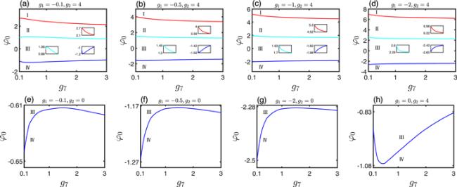
Figure 4. (a)–(d) Intervals of existence of various wave structures as a function of g7 and φ0 with different g1: (a) g1 = − 0.1, (b) g1 = − 0.5, (c) g1 = − 1, (d) g1 = − 2. Here, g2 = 4. (e)–(h) For the the third boundary curves with different g1 and g2: (e) g1 = − 0.1, g2 = 0, (f) g1 = − 0.5, g2 = 0, (g) g1 = − 2, g2 = 0, (h) g1 = 0, g2 = 4. |
3.4. The effect of adiabatic approximation and spatial diffusion rate on shock waves
In the above subsections, we discussed the shock waves under the adiabatic approximation and taking the spatial diffusion rate g8 = 0. In this subsection we will consider the effect of the non-adiabatic approximation and spatial diffusion on shock waves by solving equations (3 ) and (4 ). Here, we select g1 = − 1, g2 = 4, g5 = 1, g7 = 1 and g8 = − 5.
In figure 5, the profiles of shock waves are shown after considering the time-dependent reservoir density and its spatial diffusion. When $\tfrac{\partial n}{\partial \tau }\ne 0$ and g8 = 0 some small oscillations occur at the trailing waves as shown in figures 5(a) and 5(b). In figure 5(c), the amplitude of the rarefaction wave increases. That is, the time-dependent density is unfavorable for generating shock waves. However, after taking the spatial diffusion g8 = − 5, we find the small oscillations and amplified amplitude are effectively suppressed, as shown in figures 5(d)–(f), and these profiles are similar to those in figures 1(a)–(c). So, the results obtained in the above subsections are reliable. However, we also find that the platforms separating the two shock waves are different. After considering $\tfrac{\partial n}{\partial \tau }\ne 0$ and g8 = 0, the platform becomes flat. However, taking $\tfrac{\partial n}{\partial \tau }\ne 0$ and g8 = − 5 it will become steeper. In figures 5(g)–(i), the formation processes of shock waves in figures 5(d)–(f) are shown.

Figure 5. The profiles of various shock waves after considering the non-adiabatic approximation and spatial diffusion: (a)–(c) for $\tfrac{\partial n}{\partial \tau }\ne 0$ and g8 = 0, (d)–(f) for $\tfrac{\partial n}{\partial \tau }\ne 0$ and g8 = − 5. (g)–(i) The projection of the formation process for shock waves in figures (d)–(f). |
4. Summary
In summary, we have generated the supersonic shock waves by inputting a piecewise constant wave in a nonresonant pumped exciton–polariton condensate and found the parameter regions of various waves, which can be used to control shock waves. The regions of existence can be controlled by self-interaction, cross-interaction, intensity of pumping, condensation rate and spatial diffusion of the reservoir density. Compared with the previous studies, we not only have obtained various novel shock waves in the incoherent pumped polariton condensates but also have extended the range of existence of shock waves, from Kerr nonlinearity to mixed nonlinearity and from a weak dispersion system to a normal dispersion system. The results presented here may be useful for understanding the physical properties of condensates out of equilibrium and guiding the experimental study of condensate shock waves, which may have potential applications in polariton condensates for information storage and processing or quantum simulators.