


1. Introduction
Rogue waves are sudden large displacements in a calm situation which can be observed in the ocean [1]. Modern research also finds that rogue waves exist in optical fiber propagation [2, 3], plasma physics [4], atmospheric science [5] and the financial sector [6], etc. It appears for a short time with high amplitude and is extremely destructive, so it is significant to study the properties of rogue wave solutions. A rogue wave solution as a rational solution of a nonlinear wave equation is localized in both space and time [7]. In the field of mathematical research, the first-order rogue waves were observed in the nonlinear Schrödinger equation for the first time [8]. In recent years, high-order rogue waves have been obtained through Darboux transformation [9–11] or Kadomtsev-Petviashvili hierarchy reduction [12, 13] in some articles, the transformations of the above methods are complex [14] and the calculation is difficult, therefore, generating high-order rogue waves directly from N-solitons without complex transformations is worth studying.
As we all know, Hirota’s bilinear method [15] is a direct method in the field of integrable systems to obtain N-soliton solutions. Based on the N-soliton solutions [16], different types of solutions such as line waves and breather waves [17, 18] can be constructed by restricting the parameters. One application is the long-wave limit method introduced by Ablowitz [19], which is suitable for solving the rational solutions of nonlinear evolution equations (NLEEs) [20, 21]. Due to the generality of the method, different types of rational solutions have been obtained. In our team, higher-order smooth positons and breather positons have been obtained by taking the limit of the phase parameters [22–24]. After that, an improved long-wave limit method is proposed to generate high-order rogue waves in (1+1)-dimensional NLS equation [25]. Compared with the traditional long-wave limit method, the improved limit method can be used to solve high-order rogue waves of (1+1)-dimensional equations. Furthermore, the rogue wave solutions of the (3+1)-KdV-BBM equation are generated through the improved limit method [26]. In multi-component systems, rogue waves also can be simultaneously excited using simple initial conditions in the form of a plane wave with a small amplitude single-peak perturbation [27].
In this paper, we consider the (3+1)-dimensional Kadomtsev-Petviashvili (KP) equation [28, 29],1 ) are revealed by a symbolic computation approach that involves polynomial calculations. In [34], the rogue wave solutions of (3+1)-dimensional KP are also solved by an algebraic method. Therefore, our method of deriving rogue wave solutions by taking the limit of phase parameters is completely different from the above approaches.
$\begin{eqnarray}{({u}_{t}+\delta {{uu}}_{x}+\mu {u}_{{xxx}})}_{x}+\chi ({u}_{{xx}}+{u}_{{yy}}+{u}_{{zz}})=0,\end{eqnarray}$ 
where δ, μ and χ are parameters, u is a wave amplitude function of {x, y, z, t}. The (3+1)-dimensional KP equation has been extensively studied in many fields, it can be used to research hydrodynamics [30], plasma physics [31, 32], the dynamical behavior of nonlinear waves [33], etc. Therefore, studying the solutions of the (3+1)-dimensional KP equation is meaningful. In [28], rogue wave solutions of equation (In this paper, based on the N-solitons of Hirota’s bilinear method, the first-order rogue wave solutions can be generated by applying the long-wave limit method. Further, second-order and third-order rogue waves can be derived from the N-soliton solutions by reconstructing the phase parameters. Moreover, different patterns of rogue waves are generated by controlling the introduced parameters. At the last, we summarize how to generate the N-order rogue wave solutions.
2. First-order rogue wave
In this section, we use the traditional long-wave limit method to derive the first-order rogue wave solution from a two-soliton solution, and then we discuss the profile of the solutions. In order to get the rogue waves from the N-solitons, we set ξ = x + dy − et, η = z [28] of equation (1 ), then3 ) into (2 ), the Hirota bilinear form can be obtained as follows:4 ) admits solutions as follows:
$\begin{eqnarray}\mu {u}_{\xi \xi \xi \xi }+\left({d}^{2}\chi +\chi -e\right){u}_{\xi \xi }+\displaystyle \frac{1}{2}\delta {\left({u}^{2}\right)}_{\xi \xi }+\chi {u}_{\eta \eta }=0.\end{eqnarray}$ 
Considering Hirota’s bilinear method, give the following variable transformation $\begin{eqnarray}u={u}_{0}+\displaystyle \frac{12\mu }{\delta }{(\mathrm{ln}f)}_{\xi \xi },\end{eqnarray}$ 
where u0 is a constant and f = f(ξ, η) is the auxiliary function. Substituting ( $\begin{eqnarray}(\mu {D}_{\xi }^{4}+\gamma {D}_{\xi }^{2}+\chi {D}_{\eta }^{2})f\cdot f=0,\end{eqnarray}$ 
where γ = (d2 + 1)χ − e + δu0. Based on Hirota’s bilinear method, equation ( $\begin{eqnarray}{f}_{N}=\displaystyle \sum _{\tau =0,1}\exp \left(\displaystyle \sum _{j=1}^{N}{\tau }_{i}{\varphi }_{i}+\displaystyle \sum _{1\leqslant j\lt i\leqslant N}^{N}{\tau }_{i}{\tau }_{j}{A}_{{ij}}\right),\end{eqnarray}$ 
with $\begin{eqnarray*}\begin{array}{l}{\varphi }_{i}={p}_{i}\xi +{q}_{i}\eta +\mathrm{ln}({\zeta }_{i0}),\,\,{q}_{i}={\sigma }_{i}{\left(-\chi \right)}^{-\tfrac{1}{2}}{p}_{i}\sqrt{\mu {p}_{i}^{2}+\gamma },\\ \exp ({A}_{{ij}})=\displaystyle \frac{\chi {\left({q}_{i}-{q}_{j}\right)}^{2}+(\gamma -\delta ){\left({p}_{i}-{p}_{j}\right)}^{2}-\mu {\left({p}_{i}-{p}_{j}\right)}^{4}}{\chi {\left({q}_{i}+{q}_{j}\right)}^{2}+(\gamma -\delta ){\left({p}_{i}+{p}_{j}\right)}^{2}-\mu {\left({p}_{i}+{p}_{j}\right)}^{4}},\end{array}\end{eqnarray*}$ 
the sum takes all the possible combinations of τi = 0, 1 (i = 1, 2, ⋯ ,N), and ζi0, pi, qi(i = 1, 2, ⋯ ,N) are free parameters, σi = ± 1(i = 1, 2, ⋯ ,N). Based on the above content, we discuss how to obtain rogue wave solutions from N-soliton solutions by the direct limit method.For N = 2, based on Hirota’s bilinear method, the two-soliton solution can be expressed as5 ). In order to generate the rogue wave solutions, setting p1 = P1 ε, p2 = P2 ε, σ1 = 1, σ2 = − 1, when ε → 0, then we have7 ), the coefficient of ε2 is obtained as follows:8 ) into the transformation (3 ), then the fundamental first-order rogue wave solution of the (3+1)-dimensional KP can be expressed as
$\begin{eqnarray}{f}_{2}=1+\exp ({\varphi }_{1})+\exp ({\varphi }_{2})+\exp ({\varphi }_{1}+{\varphi }_{2}+{A}_{12}),\end{eqnarray}$ 
where φ1, φ2 and A12 are determined by equation ( $\begin{eqnarray}\begin{array}{rcl}{f}_{2} & = & ({\zeta }_{10}+1)({\zeta }_{20}+1)\\ & & +\,\left[({P}_{1}{\zeta }_{10}+{P}_{2}{\zeta }_{20}+({P}_{1}+{P}_{2}){\zeta }_{10}{\zeta }_{20})\xi \right.\\ & & +\,{\chi }^{-1}\sqrt{-\chi \gamma }({P}_{1}{\zeta }_{10}-{P}_{2}{\zeta }_{20}\\ & & \left.+\,({P}_{1}-{P}_{2}){\zeta }_{10}{\zeta }_{20})\eta \right]\epsilon +o({\epsilon }^{2}).\end{array}\end{eqnarray}$ 
Setting the coefficients of ε0 and ε1 as zero, then the undetermined phase parameters ζ10 and ζ20 can be solved as ζ10 = ζ20 = −1. Substituting them into equation ( $\begin{eqnarray}{f}_{2}={P}_{1}{P}_{2}\left({\xi }^{2}+\gamma {\chi }^{-1}{\eta }^{2}-3\mu {\gamma }^{-1}\right).\end{eqnarray}$ 
Substituting equation ( $\begin{eqnarray}u={u}_{0}+\displaystyle \frac{24{\gamma }^{2}\mu (-{\xi }^{2}+\gamma {\chi }^{-1}{\eta }^{2}-3\mu )}{\delta {\left(\gamma {\xi }^{2}+{\gamma }^{2}{\chi }^{-1}{\eta }^{2}+3\mu \right)}^{2}}.\end{eqnarray}$ 
Setting the parameters $\begin{eqnarray}{u}_{0}=1,d=1,e=1,\chi =-1,\delta =1,\mu =1,\end{eqnarray}$ 
then the first-order rogue wave solution is shown in figure 1.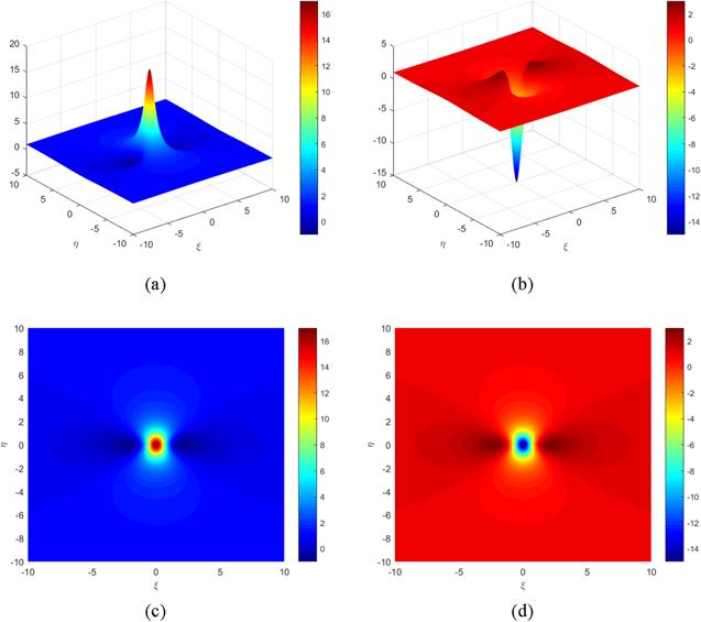
Figure 1. First-order rogue wave solution. Bright rogue wave solution with parameters ( |
In the following, we analyze the profile and type of the first-order fundamental rogue wave solutions. The solution equation (9 ) is determined by five free parameters{d, e, χ, δ, μ}, when u0 = 1. In order to ensure the rogue wave solutions are non-singular, these free parameters must satisfy the following two constraints, one is {χ < 0, μ > 0, γ < 0}, the other is {χ > 0, μ < 0, γ > 0}. Under the above parameter constraints, bright rogue wave solutions are generated when δ and μ have opposite signs, see figure 1(a). Contrariwise, dark rogue wave solutions are shown when δ and μ have the same sign, see figure 1(b). Furthermore, the amplitude and width of the rogue waves are affected by the parameters. When ∣χ∣ increases, the amplitude of the rogue wave will increase gradually; when ∣δ∣ increases, the wave amplitude will decrease gradually; when ∣μ∣ increases, the width of the rogue wave will increase and the amplitude remains constant. Meanwhile, the parameters d2 and e have the same effect on the profile, that is the amplitude of the bright rogue wave will increase gradually as e increases, and the dark rogue wave has the opposite effect. All the effects of different free parameters on amplitude and width are shown in figure 2.

Figure 2. Profile of first-order rogue wave solution. (a) With parameters ( |
3. Second-order rogue wave
In this section, we extend the traditional long-wave limit method to generate second-order rogue wave solutions directly. By adding perturbation to the phase parameters, rational rogue wave solutions can be derived by taking a series of N-soliton solutions. Moreover, the general expression of the perturbation parameters is given in the following discussion. Without loss of generality, setting u0 = 1, d = 1, e = 1, χ = − 1, δ = 1, μ = 1.
For N = 4, the soliton solution is as follows:5 ).
$\begin{eqnarray}\begin{array}{rcl}{f}_{4} & = & 1+\displaystyle \displaystyle \sum _{i=1}^{4}\exp ({\varphi }_{i})+\displaystyle \displaystyle \sum _{i\lt j}^{4}\exp ({\varphi }_{i}+{\varphi }_{j}+{A}_{{ij}})\\ & & +\,\displaystyle \sum _{i\lt j\lt k}^{4}\exp ({\varphi }_{i}+{\varphi }_{j}+{\varphi }_{k}+{A}_{{ij}}+{A}_{{ik}}+{A}_{{jk}})\\ & & +\,\exp \left(\displaystyle \displaystyle \sum _{i=1}^{4}{\varphi }_{i}+\displaystyle \sum _{i\lt j}^{4}{A}_{{ij}}\right),\end{array}\end{eqnarray}$ 
setting φi as $\begin{eqnarray}{\varphi }_{i}={p}_{i}\xi +{q}_{i}\eta +\mathrm{ln}({\zeta }_{i0})+{\zeta }_{i2}{\epsilon }^{2}+{\zeta }_{i3}{\epsilon }^{3},\end{eqnarray}$ 
and other parameters remain constant in equation (Firstly, we consider the case of ζi3 = 0. In order to generate the rogue waves, setting p1 = P1ε, p2 = P2ε, p3 = P3ε, p4 = P4ε, σ1 = σ2 = 1, σ3 = σ4 = − 1, substituting them into equation (11 ) and taking series of ε, when ε → 0, f4 can be expressed as the series expansion14 ) into equation (13 ), and then the coefficient of ε6 is expressed as follows:
$\begin{eqnarray}{f}_{4}=\displaystyle \sum _{i=0}^{6}{f}_{4}^{(i)}{\epsilon }^{i}+o({\epsilon }^{7}).\end{eqnarray}$ 
Setting the coefficients of ε0, ⋯ ,ε5 equal to zero, that is $\{{f}_{4}^{(0)}=0,{f}_{4}^{(1)}=0\,{f}_{4}^{(2)}=0,{f}_{4}^{(3)}=0,{f}_{4}^{(4)}=0,{f}_{4}^{(5)}=0\}$. Solving the equations, ζi0 and ζi2 are obtained as follows: $\begin{eqnarray}\begin{array}{rcl}{\zeta }_{10} & = & -{\zeta }_{20}=\displaystyle \frac{{P}_{1}+{P}_{2}}{{P}_{1}-{P}_{2}},{\zeta }_{30}=-{\zeta }_{40}=\displaystyle \frac{{P}_{3}+{P}_{4}}{{P}_{3}-{P}_{4}},\\ {\zeta }_{12} & = & {\zeta }_{22}=\displaystyle \frac{{P}_{1}{P}_{2}}{12},{\zeta }_{32}={\zeta }_{42}=\displaystyle \frac{{P}_{3}{P}_{4}}{12},\end{array}\end{eqnarray}$ 
where P1 ≠ P2, P3 ≠ P4. Substituting parameter constraints ( $\begin{eqnarray}\begin{array}{rcl}{f}_{4} & = & \displaystyle \frac{1}{288}\left\{{P}_{1}{P}_{2}{P}_{3}{P}_{4}({P}_{1}+{P}_{2})({P}_{3}+{P}_{4})(8{\xi }^{6}\right.\\ & & +(48{\eta }^{2}+100){\xi }^{4}\\ & & +\left(96{\eta }^{4}+720{\eta }^{2}-250\right){\xi }^{2}\\ & & \left.+64{\eta }^{6}+272{\eta }^{4}+1900{\eta }^{2}+1875)\right\},\end{array}\end{eqnarray}$ 
f4 can form the fundamental pattern of second-order rogue wave solutions, see figure 3.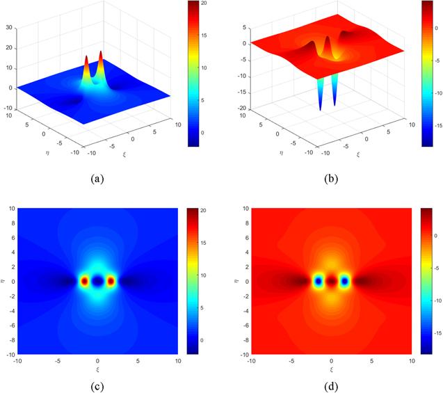
Figure 3. Second-order fundamental rogue wave solution with ζi3 = 0. Bright rogue wave solution with parameters ( |
Suppose ζi3 ≠ 0. Substituting equation (14 ) into equation (13 ), and solving the equations $\{{f}_{4}^{(0)}\,=0,{f}_{4}^{(1)}=0\,{f}_{4}^{(2)}=0,{f}_{4}^{(3)}=0,{f}_{4}^{(4)}=0,{f}_{4}^{(5)}=0\}$,the parameters ζi3 are calculated:16 ) into equation (13 ), then the coefficient of ε6 is expressed as15 ). f4trig can form the triangle pattern of second-order rogue wave solutions with ζ43, see figure 4. As ζ43 becomes larger, the bound state of second-order rogue wave will gradually disperse to three individual rogue waves, see figure 5.
$\begin{eqnarray}\left\{{\zeta }_{13}={\zeta }_{23}=\displaystyle \frac{{P}_{1}{P}_{2}({P}_{1}+{P}_{2})}{{P}_{3}{P}_{4}({P}_{3}+{P}_{4})}\,{\zeta }_{43},{\zeta }_{33}={\zeta }_{43}\right\},\end{eqnarray}$ 
where ζ43 is an arbitrary parameter. Substituting equation ( $\begin{eqnarray}\begin{array}{l}{f}_{4{trig}}={f}_{4}+\displaystyle \frac{1}{288}\displaystyle \frac{{P}_{1}{P}_{2}({P}_{1}+{P}_{2})}{{P}_{3}{P}_{4}\left({P}_{3}+{P}_{4}\right)}\\ \quad \times \left(1152{\zeta }_{43}^{2}-({P}_{3}^{2}{P}_{4}+{P}_{3}{P}_{4}^{2})\right.\\ \quad \left.\times (18{\eta }^{2}\xi -192{\xi }^{3}+96\xi ){\zeta }_{43}\right),\end{array}\end{eqnarray}$ 
where f4 is equation (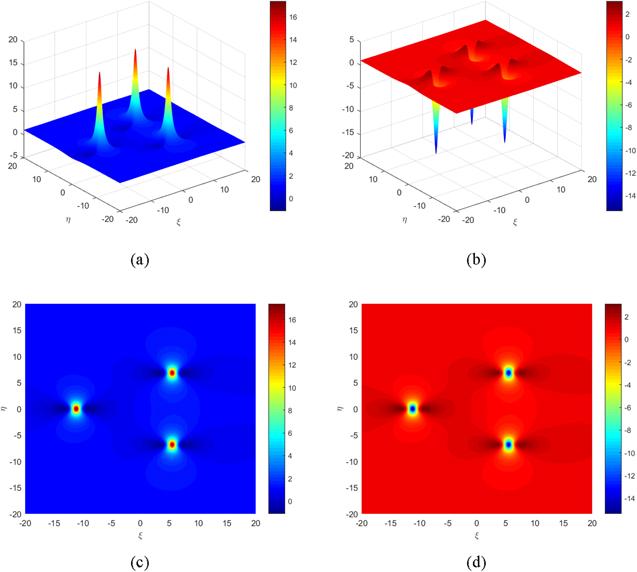
Figure 4. Second-order triangle rogue wave solution with ζ43 = 10000. Bright rogue wave solution with parameters ( |
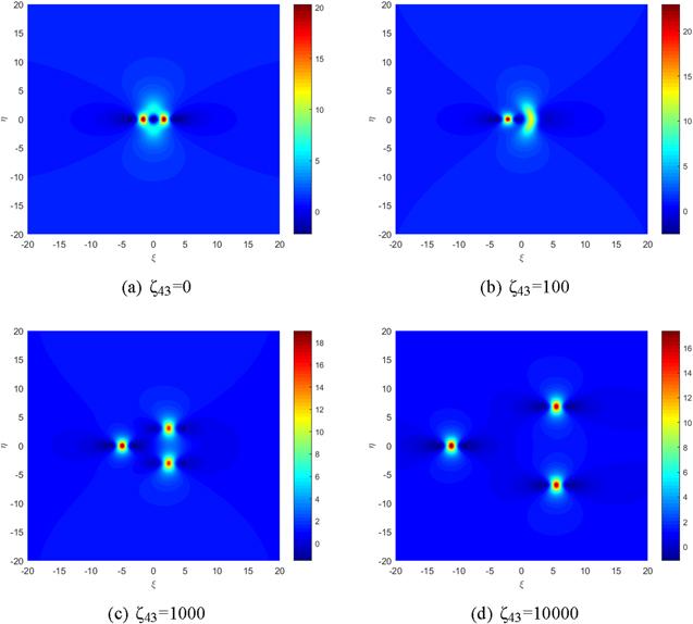
Figure 5. Evolution of second-order rogue wave solutions with different ζ43. |
4. Third-order rogue wave
In this section, we proceed to solve the third-order rogue wave solutions through the pretty direct limit approach. For N = 6, the bilinear equation is18 ). When ε → 0, f6 can be expressed as the following series21 ) into equation (20 ), setting P1 = P6 = 1, P2 = P5 = 2, P3 = P4 = 3, then the coefficient of ε12 is expressed as follows:
$\begin{eqnarray}\begin{array}{rcl}{f}_{6} & = & 1+\displaystyle \displaystyle \sum _{i=1}^{6}\exp ({\varphi }_{i})+\displaystyle \displaystyle \sum _{i\lt j}^{6}\exp ({\varphi }_{i}+{\varphi }_{j}+{A}_{{ij}})\\ & & +\displaystyle \displaystyle \sum _{i\lt j\lt k}^{6}\exp ({\varphi }_{i}+{\varphi }_{j}+{\varphi }_{k}+{A}_{{ij}}+{A}_{{ik}}+{A}_{{jk}})\\ & & +\displaystyle \displaystyle \sum _{i\lt j\lt k\lt l}^{6}\exp ({\varphi }_{i}+{\varphi }_{j}+{\varphi }_{k}+{\varphi }_{l}\\ & & +{A}_{{ij}}+{A}_{{ik}}+{A}_{{il}}+{A}_{{jk}}+{A}_{{jl}}+{A}_{{kl}})\\ & & +\displaystyle \displaystyle \sum _{i\lt j\lt k\lt l\lt s}^{6}\exp ({\varphi }_{i}+{\varphi }_{j}+{\varphi }_{k}+{\varphi }_{l}+{\varphi }_{s}+{A}_{{ij}}\\ & & +{A}_{{ik}}+{A}_{{il}}+{A}_{{is}}+{A}_{{jk}}+{A}_{{jl}}+{A}_{{js}}\\ & & +{A}_{{kl}}+{A}_{{ks}}+{A}_{{ls}})\\ & & +\exp \left(\displaystyle \displaystyle \sum _{i=1}^{6}{\varphi }_{i}+\displaystyle \sum _{i\lt j}^{6}{A}_{{ij}}\right),\end{array}\end{eqnarray}$ 
rewrite $\begin{eqnarray}{\varphi }_{i}={p}_{i}\xi +{q}_{i}\eta +\mathrm{ln}({\zeta }_{i0})+{\zeta }_{i2}{\epsilon }^{2}+{\zeta }_{i3}{\epsilon }^{3}+{\zeta }_{i4}{\epsilon }^{4}+{\zeta }_{i5}{\epsilon }^{5}.\end{eqnarray}$ 
Setting pi = Piε, (i = 1, 2, ⋯ ,6), σ1 = σ2 = σ3 = 1, σ4 = σ5 = σ6 = −1, substituting the parameters into equation ( $\begin{eqnarray}{f}_{6}=\displaystyle \sum _{i=0}^{12}{f}_{6}^{(i)}{\epsilon }^{i}+o({\epsilon }^{13}).\end{eqnarray}$ 
Firstly, suppose ζi3 = ζi5 = 0, setting the coefficients of ε0, ⋯ ,ε11 equal to zero, that is $\{{f}_{6}^{(i)}=0,i\,=\,1,2,\cdots ,11\}$. Solving the equations, ζi0, ζi2 and ζi4 are obtained as follows: $\begin{eqnarray}\begin{array}{rcl}{\zeta }_{10} & = & -\displaystyle \frac{({P}_{1}+{P}_{2})({P}_{1}+{P}_{3})}{({P}_{1}-{P}_{2})({P}_{1}-{P}_{3})},\\ {\zeta }_{20} & = & \displaystyle \frac{({P}_{1}+{P}_{2})({P}_{2}+{P}_{3})}{({P}_{1}-{P}_{2})({P}_{2}-{P}_{3})},\\ {\zeta }_{30} & = & -\displaystyle \frac{({P}_{1}+{P}_{3})({P}_{2}+{P}_{3})}{({P}_{1}-{P}_{3})({P}_{2}-{P}_{3})},\\ {\zeta }_{40} & = & -\displaystyle \frac{({P}_{4}+{P}_{5})({P}_{4}+{P}_{6})}{({P}_{4}-{P}_{5})({P}_{4}-{P}_{6})},\\ {\zeta }_{50} & = & \displaystyle \frac{({P}_{4}+{P}_{5})({P}_{5}+{P}_{6})}{({P}_{4}-{P}_{5})({P}_{5}-{P}_{6})},\\ {\zeta }_{60} & = & -\displaystyle \frac{({P}_{4}+{P}_{6})({P}_{5}+{P}_{6})}{({P}_{4}-{P}_{6})({P}_{5}-{P}_{6})},\\ {\zeta }_{12} & = & {\zeta }_{22}=\displaystyle \frac{{P}_{1}{P}_{2}}{12},{\zeta }_{32}=\displaystyle \frac{{P}_{3}({P}_{1}+{P}_{2}-{P}_{3})}{12},\\ {\zeta }_{42} & = & {\zeta }_{52}=\displaystyle \frac{{P}_{4}{P}_{5}}{12},{\zeta }_{62}=\displaystyle \frac{{P}_{6}({P}_{4}+{P}_{5}-{P}_{6})}{12},\\ {\zeta }_{14} & = & {\zeta }_{24}={\zeta }_{34}=-\displaystyle \frac{7{P}_{1}{P}_{2}{P}_{3}({P}_{1}{P}_{2}+{P}_{1}{P}_{3}+{P}_{2}{P}_{3})}{144({P}_{1}+{P}_{2}+{P}_{3})},\\ {\zeta }_{44} & = & {\zeta }_{54}={\zeta }_{64}=-\displaystyle \frac{7{P}_{4}{P}_{5}{P}_{6}({P}_{4}{P}_{5}+{P}_{4}{P}_{6}+{P}_{5}{P}_{6})}{144({P}_{4}+{P}_{5}+{P}_{6})},\end{array}\end{eqnarray}$ 
where P1 ≠ P2 ≠ P3, P4 ≠ P5 ≠ P6. Substituting equation ( $\begin{eqnarray}\begin{array}{l}{f}_{6}=\displaystyle \frac{1}{576}\left\{36864{\eta }^{12}+(110592{\xi }^{2}+534528){\eta }^{10}\right.\\ \quad +(138240{\xi }^{4}+2626560{\xi }^{2}+9987840){\eta }^{8}+(92160{\xi }^{6}\\ \quad +3363840{\xi }^{4}+40803840{\xi }^{2}+153404160){\eta }^{6}\\ \quad +(34560{\xi }^{8}+1774080{\xi }^{6}+21571200{\xi }^{4}-4233600{\xi }^{2}\\ \quad +786802800){\eta }^{4}+(6912{\xi }^{10}+397440{\xi }^{8}+5362560{\xi }^{6}\\ \quad +31752000{\xi }^{4}+40748400{\xi }^{2}+3610761000){\eta }^{2}\\ \quad +576{\xi }^{12}+28224{\xi }^{10}+105840{\xi }^{8}+1811040{\xi }^{6}\\ \quad \left.-62254500{\xi }^{4}+958719300{\xi }^{2}+878826025\right\},\end{array}\end{eqnarray}$ 
f6 can generate the fundamental pattern of third-order rogue wave solutions, see figure 6. The parameters ζi2 and ζi4 are used to ensure the existence of the third-order rogue wave solutions.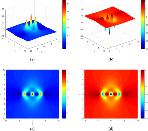
Figure 6. Third-order fundamental rogue wave solution with ζi3 = ζi5 = 0. Bright rogue wave solution with parameters ( |
For the case ζi5 = 0. Based on equation (21 ), solving the equations $\{{f}_{6}^{(i)}=0,i=1,2,\cdots ,11\}$, the parameters ζi3 are obtained as follows:20 ), then the triangle pattern of third-order rogue waves is generated, see figure 7. The patterns of the rogue waves are controlled by the introduced parameter ζ63. Through increasing ζ63, the triangle rogue wave gradually expands which consists of six individual rogue waves.
$\begin{eqnarray}\begin{array}{l}\left\{{\zeta }_{23}=2{\zeta }_{13}+{\zeta }_{53}-2{\zeta }_{63},{\zeta }_{33}=3{\zeta }_{13}\right.\\ \quad \left.+4{\zeta }_{53}-8{\zeta }_{63},{\zeta }_{43}=4{\zeta }_{53}-5{\zeta }_{63}\right\}\end{array}\end{eqnarray}$ 
with free parameters ζ13, ζ53, ζ63. Setting ζ13 = ζ53 = 0, substituting the parameters’ relationship into equation (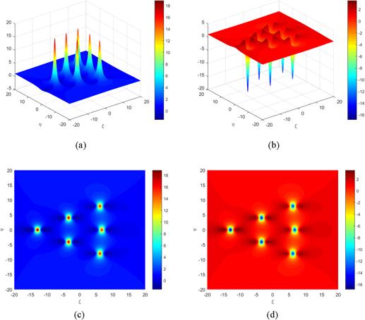
Figure 7. Third-order triangle rogue wave solution with ζ63 = 100. Bright rogue wave solution with parameters ( |
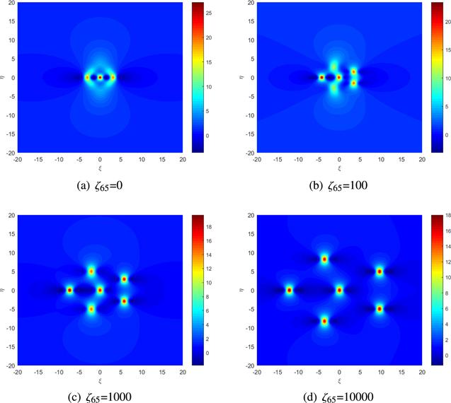
For the case ζi3 = 0. The parameters ζi5 are obtained through a similar approach:20 ), then we obtain the pentagon patterns of third-order rogue waves, see figure 8. The role of the parameter ζ65 is also to control the pattern of the third-order rogue waves. Through increasing the parameter ζ65, the bound state of the third-order pentagon rogue wave will gradually disperse to six individual rogue waves. The effects of ζ63 and ζ65 on the rogue waves are shown in figures 9 and 10.
$\begin{eqnarray}\{{\zeta }_{35}=-5{\zeta }_{15}+4{\zeta }_{25}+5{\zeta }_{65}\}\end{eqnarray}$ 
with free parameters ζ15, ζ25, ζ45, ζ55, ζ65. Setting ζ15 = ζ25 = 0, ζ45 = ζ55 = 1, substituting the parameter limitations into equation (
Figure 8. Third-order pentagon rogue wave solution with ζ65 = 10000. Bright rogue wave solution with parameters ( |

Figure 9. Evolution of third-order triangle rogue wave solutions with different ζ63. |
Figure 10. Evolution of third-order pentagon rogue wave solutions with different ζ65. |
More generally, the N-order rogue wave solution can also be generated from the 2N-soliton solution:
$\begin{eqnarray}{f}_{2N}=\displaystyle \sum _{\tau =0,1}\exp \left(\displaystyle \sum _{j=1}^{(2N)}{\tau }_{i}{\varphi }_{i}+\displaystyle \sum _{1\leqslant j\lt i\leqslant 2N}^{(2N)}{\tau }_{i}{\tau }_{j}{A}_{{ij}}\right),\end{eqnarray}$ 
rewrite $\begin{eqnarray}\begin{array}{rcl}{\varphi }_{i} & = & {p}_{i}\xi +{q}_{i}\eta +\mathrm{ln}({\zeta }_{i0})+{\zeta }_{i2}{\epsilon }^{2}\\ & amp; & +{\zeta }_{i3}{\epsilon }^{3}+\cdots +{\zeta }_{i2N-1}{\epsilon }^{2N-1},\end{array}\end{eqnarray}$ 
substituting φi into the Hirota soliton solution, by applying limits to fN and taking series of ε, then we get $\begin{eqnarray}{f}_{2N}=\displaystyle \sum _{i=0}^{N(N+1)}{f}_{2N}^{(i)}{\epsilon }^{i}+o({\epsilon }^{N(N+1)+1}).\end{eqnarray}$ 
Solving the coefficients of εi (i = 0, 1, 2, ⋯ ,N(N + 1) − 1), that is $\{{f}_{2N}^{(i)}=0,i\,=\,0,1,2,\cdots ,N(N+1)-1\}$. Then the coefficient of εN(N+1) is the N-order rogue wave solution, which is a polynomial solution with degree N(N + 1).5. Conclusion
In this paper, based on Hirota’s bilinear method, rogue wave solutions of (3+1)-dimensional KP equation are derived from N-solitons. We reconstruct the phase parameters and take long wave limits, then the rogue wave solutions can be generated and expressed explicitly in rational forms. The first-order rogue wave solutions are generated by 2-degree rational polynomial functions. Then we analyse the profile of the first-order rogue wave solutions, such as bright-dark, amplitude and width. The second-order rogue wave solutions are produced by 6-degree rational polynomial functions. The introduced parameter ζi3 controls the patterns of the second-order rogue wave solutions. When ζi3 = 0, the solution is a fundamental pattern; when ζi3 ≠ 0, there is a triangle pattern. Furthermore, the third-order rogue wave solutions are generated by 12-degree rational polynomial functions. The patterns of the rogue waves are also determined by some introduced free parameters. When the parameters ζi3 = ζi5 = 0, the solution is a fundamental pattern; when ζi3 = 0, ζi5 ≠ 0, there is a pentagon pattern; when ζi3 ≠ 0, ζi5 = 0, there is a triangle pattern. In the end, the N-order rogue wave solutions are summarized. We hope that our method can be applied to solve rogue wave solutions of other nonlinear wave equations and the results are helpful to the study of rogue waves.