


1. Introduction
In conservative systems, soliton is generally a localized-wave packet arising from the balance between nonlinearity, dispersion and/or diffraction, which has been observed in many branches of nonlinear physics such as Bose–Einstein condensates [1–5] and optics [6–8]. However, in reality many systems have energy exchange with the environment, i.e. they are of dissipative. In such systems, dissipative soliton is principally a fundamental extension of conventional soliton, whose formation arises from an additional balance between gain and loss [9–11]. In past, dissipative solitons have attracted great research interest and have been realized in various optical platforms such as mode-locked lasers [11–15], passive fiber cavities [16–18] and optical microresonators [19, 20]. Unlike the conservative case, in which a given set of system parameters generally lead to an infinite number of soliton solutions, a given dissipative model only has a fixed soliton solution being associated with attractor. A strong attractor means the fixed soliton solution has a high degree of stability.
Generally, the most well-known dissipative models are the complex Ginzburg–Landau equation [11, 21–23] and the Lugiato–Lefever equation [24, 25], which are usually used to describe the formations of the mode-locking soliton and the dissipative cavity soliton, respectively. However, the above two equations are non-integral, which means no general analytical solutions exist. That brings difficulties for the theoretical analysis of soliton attractors. Therefore, finding some analytical solutions of dissipative model is very meaningful for the study of dissipative-soliton dynamics. Recently, analytical solutions for the nonlinear Schrödinger equation (NLSE) with a simplified dissipative perturbation have been found, resulting in nontrivial monosolitonic fixed point attractor patterns [26]. This raises a natural question: how do soliton attractors behave when considering coupling effects in the dissipative model of [26], given the universality of multi-component systems?
In this work, we generalize the Lagrangian perturbation theory to two-component coupled systems and analyze the attractor features of the soliton solutions. The coupled NLSEs have familiar exact soliton solutions, including bright-bright soliton, dark–dark soliton and dark-bright soliton [27–31]. We establish the dissipation-perturbed coupled NLSEs and adopt the bright-bright soliton as a trial function. The specific dissipative soliton solutions are solved using the Lagrangian perturbation theory, and their attractor features are numerically demonstrated. We find that the introduction of coupling effect brings more interesting properties to soliton attractors.
2. The coupled model with dissipation effects
We consider the perturbed coupled NLSEs in the form1 ) and (2 ) are known to exert viscous friction forces to solitons [35] as well as increase their amplitudes without making changes in their velocity. Considering solitons’ ability to oscillate around the minima of an external conservative potential [26, 36], we believe such dissipative perturbation will make solitons resting at any minimum of conservative part of perturbation [37]. So we can use Lagrangian perturbation theory to analyze dynamical behaviors of coupled solitons in this dissipation system, when the dissipations are weak.
$\begin{eqnarray}{\rm{i}}{u}_{t}+{u}_{{xx}}+2(| u{| }^{2}+g| v{| }^{2})u=\epsilon R(u),\end{eqnarray}$
$\begin{eqnarray}{\rm{i}}{v}_{t}+{v}_{{xx}}+2(| v{| }^{2}+g| u{| }^{2})v=\epsilon R(v),\end{eqnarray}$
where R(u) = i(A1uxx + B1u) and R(v) = i(A2vxx + B2v) denote the dissipations in the coupled systems. The subscripts denotes the derivatives with respect to the variables. For $g=\tfrac{2}{3}$, it represents the system of linearly birefringent fibers, g = 2 represents circularly birefringent fibers [32], g = 0 represents two uncoupled NLSE and g = 1 represents Manakov equations [33, 34]. ε is a parameter characterizing the perturbation. The perturbation terms in the right-hand-side of equation (To find the existence of solitonic attractors, it is necessary to analyze the dynamical evolution trajectories of coupled solitons. We focus on the situation of g = 1 and ε is small enough, since this coupling system in this case can be seen as nearly integrable system [38, 39]. We assume u(x, t) and v(x, t) are soliton solutions of the coupled NLSEs (1 )–(2 ), which can be written as
$\begin{eqnarray}u(x,t)={a}_{1}{\rm{sech}} [w(x-q)]\exp [{\rm{i}}\xi (x-q)+{\rm{i}}{\sigma }_{1}],\end{eqnarray}$
$\begin{eqnarray}v(x,t)={a}_{2}{\rm{sech}} [w(x-q)]\exp [{\rm{i}}\xi (x-q)+{\rm{i}}{\sigma }_{2}],\end{eqnarray}$
where aj and σj represent soliton amplitudes and phases, respectively, q denotes the soliton’s center position, w is the inverse of soliton width, and ξ is related with the velocity of coupled solitons.3. The fixed point attractor patterns of coupled solitons
3.1. The Lagrangian perturbation theory of two-components coupled solitons
The Lagrangian density of this coupled system without the dissipation terms is ${ \mathcal L }=\tfrac{{\rm{i}}}{2}({u}^{* }{u}_{t}-{u}_{t}^{* }u)$$-| {u}_{x}{| }^{2}+| u{| }^{4}+\tfrac{{\rm{i}}}{2}$$({v}^{* }{v}_{t}-{v}_{t}^{* }v)-| {v}_{x}{| }^{2}+| v{| }^{4}\,+\,$2∣u∣2∣v∣2. The Lagrangian $L={\int }_{-\infty }^{+\infty }{ \mathcal L }\,{\rm{d}}x$$=\tfrac{4}{3w}({a}_{1}^{4}+{a}_{2}^{4})$$+\tfrac{2}{w}[(\xi \dot{q}\,-{\xi }^{2})({a}_{1}^{2}+{a}_{2}^{2})-({a}_{1}^{2}\dot{{\sigma }_{1}}+{a}_{2}^{2}\dot{{\sigma }_{2}})]$$-\tfrac{2w}{3}({a}_{1}^{2}+{a}_{2}^{2})+\tfrac{8}{3w}{a}_{1}^{2}{a}_{2}^{2}$. Lagrangian collective coordinates are time-dependent, and we rewrite them for typographical convenience: [a1, a2, ξ, σ1, σ2, w, q] = [y1(t), y2(t), y3(t), y4(t), y5(t), y6(t), y7(t)]. Base on the derivation of monosolitonic perturbed Euler–Lagrange equation [40], we perform it on the two-component coupling system when ∣ε∣ ≪ 1, and the evolution of yj(t) (j = 1, 2, 3, ⋯,7) can be given by the following equations:
$\begin{eqnarray}\frac{\partial L}{\partial {y}_{j}}-\frac{{\rm{d}}}{{\rm{d}}t}\frac{\partial L}{\partial \dot{{y}_{j}}}=\epsilon \left[{\int }_{-\infty }^{+\infty }\Space{0ex}{1.0ex}{0ex}(R(u)\frac{\partial {u}^{* }}{\partial {y}_{j}}\,+R(v)\frac{\partial {v}^{* }}{\partial {y}_{j}}\,\Space{0ex}{1.0ex}{0ex}){\rm{d}}x+{\rm{c}}{\rm{.}}{\rm{c}}{\rm{.}}\right],\end{eqnarray}$
where c.c. represents the complex conjugate of the previous term. In our case, R(u) = i(A1uxx + B1u), R(v) = i(A2vxx + B2v).By calculation of equation (5 ), we can obtain the ordinary differential equations of the parameters of perturbed coupling solitons:
$\begin{eqnarray}{w}^{2}={a}_{1}^{2}+{a}_{2}^{2}.\end{eqnarray}$
$\begin{eqnarray}\displaystyle \frac{{\rm{d}}}{{\rm{d}}t}\left(\displaystyle \frac{{a}_{1}^{2}}{w}\right)=\epsilon \left(2{B}_{1}\displaystyle \frac{{a}_{1}^{2}}{w}-\displaystyle \frac{2}{3}{A}_{1}{a}_{1}^{2}w-2{A}_{1}{\xi }^{2}\displaystyle \frac{{a}_{1}^{2}}{w}\right).\end{eqnarray}$
$\begin{eqnarray}\displaystyle \frac{{\rm{d}}}{{\rm{d}}t}\left(\displaystyle \frac{{a}_{2}^{2}}{w}\right)=\epsilon \left(2{B}_{2}\displaystyle \frac{{a}_{2}^{2}}{w}-\displaystyle \frac{2}{3}{A}_{2}{a}_{2}^{2}w-2{A}_{2}{\xi }^{2}\displaystyle \frac{{a}_{2}^{2}}{w}\right).\end{eqnarray}$
$\begin{eqnarray}\dot{\xi }=-\displaystyle \frac{4\xi \epsilon ({A}_{1}{a}_{1}^{2}+{A}_{2}{a}_{2}^{2})}{3}.\end{eqnarray}$
Other equations are $\dot{q}=2\xi $ and $\dot{{\sigma }_{1}}=\dot{{\sigma }_{2}}={w}^{2}+{\xi }^{2}$, which give q = 2ξt + x0 and σ1,2 = (w2 + ξ2)t + σ10,20. The x0 is the initial center position of soliton, and σ10,20 are the initial spatial-independent phases of solitons.We proceed to examine whether this system exhibits attractor patterns. It should be noted that in treating coupled solitons as classical particles, this analysis disregards the changes in shape and phases brought about by perturbations. Let’s start from equation (9 ), which determines soliton’s velocity ${v}_{c}=2\xi ={v}_{c0}\exp [-\tfrac{4\epsilon ({A}_{1}{a}_{1}^{2}+{A}_{2}{a}_{2}^{2})t}{3}]$ (vc0 = 2ξ0 is the initial velocity of soliton). When 0 < ε ≪ 1 and A1, A2 > 0, the velocity will decay with time. Namely, vc → 0 when t → +∞ .
Now we investigate equation (7 ) (8 ), the polynomials of the right hand sides of these two equations have similar forms. For the large time scale, the $\tfrac{{\rm{d}}}{{\rm{d}}t}\left(\tfrac{{a}_{1}^{2}}{w}\right)=0$, $\tfrac{{\rm{d}}}{{\rm{d}}t}\left(\tfrac{{a}_{2}^{2}}{w}\right)=0$, and ξ → 0, we have6 )). When one component of the coupled system disappears, the equations should reduce to the scalar case [26]. Therefore, a1 and a2 cannot both be zero. There are three cases to consider for equations (10 ), (11 ). In the first case, the two equations are equivalent when $\tfrac{{B}_{2}}{{A}_{2}}$=$\tfrac{{B}_{1}}{{A}_{1}}$, as ${a}_{1}^{2}+{a}_{2}^{2}=\tfrac{3{B}_{1}}{{A}_{1}}=\tfrac{3{B}_{2}}{{A}_{2}}$. In the second case, we consider single dissipative (such as A2 = B2 = 0), the amplitude of two-component satisfy ${a}_{1}^{2}+{a}_{2}^{2}=\tfrac{3{B}_{1}}{{A}_{1}}$ . In third case, when $\tfrac{{B}_{2}}{{A}_{2}}\ne \tfrac{{B}_{1}}{{A}_{1}}$ and A1, A2, B1, B2 ≠ 0, one of the soliton amplitudes is zero, such as ${a}_{1}^{2}=\tfrac{3{B}_{1}}{{A}_{1}}$ when a2 = 0, for which the component soliton will vanish.
$\begin{eqnarray}{a}_{1}[3{B}_{1}-{A}_{1}({a}_{1}^{2}+{a}_{2}^{2})]=0,\end{eqnarray}$
$\begin{eqnarray}{a}_{2}[3{B}_{2}-{A}_{2}({a}_{1}^{2}+{a}_{2}^{2})]=0,\end{eqnarray}$
where ${a}_{1}^{2}+{a}_{2}^{2}={w}^{2}$ (from equation (The findings suggest that over time, the system will eventually transform into static solitons with a constant sum of densities. Rather than the amplitude–velocity phase space, we can observe fixed point attractor patterns in $({a}_{1}^{2}+{a}_{2}^{2},{v}_{c})$ space for the coupled solitons, which differs from the case of scalar solitonic solutions [26]. However, the stationary points of ${a}_{1}^{2}$ and ${a}_{2}^{2}$ are not fixed when we vary the initial conditions. We can determine the evolution of each soliton amplitude from equations (6 ), (7 ), and (8 ), as
$\begin{eqnarray}\begin{array}{l}{\dot{a}}_{1}=\epsilon \left[\left({a}_{1}{B}_{1}-{a}_{1}{A}_{1}\displaystyle \frac{{w}^{2}}{3}-{a}_{1}{A}_{1}{\xi }^{2}\right)\left(2-\displaystyle \frac{{a}_{2}^{2}}{{w}^{2}}\right)\right.\\ \quad +\left.\displaystyle \frac{{a}_{2}^{2}}{{w}^{2}}\left({a}_{1}{B}_{2}-{a}_{1}{A}_{2}\displaystyle \frac{{w}^{2}}{3}-{a}_{1}{A}_{2}{\xi }^{2}\right)\right],\end{array}\end{eqnarray}$
$\begin{eqnarray}\begin{array}{l}{\dot{a}}_{2}=\epsilon \left[\left({a}_{2}{B}_{2}-{a}_{2}{A}_{2}\displaystyle \frac{{w}^{2}}{3}-{a}_{2}{A}_{2}{\xi }^{2}\right)\left(2-\displaystyle \frac{{a}_{1}^{2}}{{w}^{2}}\right)\right.\\ \quad \left.+\displaystyle \frac{{a}_{1}^{2}}{{w}^{2}}\left({a}_{2}{B}_{1}-{a}_{2}{A}_{1}\displaystyle \frac{{w}^{2}}{3}-{a}_{2}{A}_{1}{\xi }^{2}\right)\right].\end{array}\end{eqnarray}$
Then we can have the ordinary differential equations system about a1, a2, ξ, namely, $\dot{{a}_{1}}={a}_{1}{F}_{1}({a}_{1},{a}_{2},\xi )$, $\dot{{a}_{2}}={a}_{2}{F}_{2}({a}_{1},{a}_{2},\xi )$, and $\dot{\xi }=\xi {F}_{3}({a}_{1},{a}_{2},\xi )$, where F1, F2, F3 are polynomials of a1, a2, and ξ. The mathematical model used in this study is known as the cubic Kolmogorov system, which is similar to the models for population dynamics [41, 42], Lorenz attractor [43] and hydrodynamic attractors [44]. Here, our focus is on analyzing the solitonic attractors in the coupled system. Interestingly, the final amplitude value of the solitons only depends on the ratio of the parameters $\tfrac{{B}_{\mathrm{1,2}}}{{A}_{\mathrm{1,2}}}$ and not on the individual values of B1,2 and A1,2. Therefore, in our analysis, we will consider solitons moving under both identical and different parameter ratios.
3.2. Solitons under identical perturbation parameter ratios
To confirm our theoretical predictions, we performed numerical simulations of the original coupled NLSEs equation (1 ) and (2 ), using ten random bright-bright soliton solutions as initial conditions. The simulations were conducted with parameter values of B1 = B2, A1 = A2, ε = 0.001. The evolution of the solitons in the amplitude—velocity space is shown in figure 1. As shown in figure 1(a), the trajectories of the coupled solitons form a fixed point attractor pattern in the $({a}_{1}^{2}+{a}_{2}^{2},{v}_{c})$ space, with the attractor point matching our predicted point of $\tfrac{3{B}_{\mathrm{1,2}}}{{A}_{\mathrm{1,2}}}=1$. This indicates that the final total density of the two solitons is determined by the perturbation terms and is independent of the initial conditions.

Figure 1. (a) Represent the evolution of ten randomly initial coupled solitons (a–j) in $({a}_{1}^{2}+{a}_{2}^{2},{v}_{c})$ space under the same perturbed condition, (b) (c) denote $({a}_{1}^{2},{v}_{c})$ and $({a}_{2}^{2},{v}_{c})$ space. Ten coupled solitons in different initial states are ten different points in the $({a}_{1}^{2}+{a}_{2}^{2},{v}_{c})$ space. After a period of evolution, these ten different points converge to one fix point (0, 1) in (a). However, different initial states cannot converge to one fix point in $({a}_{1}^{2},{v}_{c})$ and $({a}_{2}^{2},{v}_{c})$ space that shown in (b), (c). The initial parameters setting for the ten lines are, a1 (a–j): 0.5, 0.5, 1.5, 2.8, 2, 3, 2.5, 2, 1.5, 0.4, a2: 0.3, 1, 1.5, 1.5, 2, 1, 1, 1, 1.5, 0.4, and the corresponding velocities are vc = 2ξ, vc: −1.2, −1, −1.4, −1.2, −0.6, 0.8, 1, 1.2, 1.4, 1. The other parameters are A1 = A2 = 3, B1 = B2 = 1, ε = 0.001. |
Furthermore, it is evident from figures 1(b) and (c) that there are no attractor patterns in $({a}_{1}^{2},{v}_{c})$ space and $({a}_{2}^{2},{v}_{c})$ space. This implies that the nonlinearity coupling alters the fixed point from the scalar NLSE case [26]. Although the final states of the two components depend on the initial conditions, they eventually reach a steady state. This is illustrated by the density evolution of the coupled solitons in figures 2(a) and (b). Furthermore, by numerically solving equations (9 ), (12 ), and (13 ), the final amplitudes and velocity of the coupled solitons can be obtained (solid lines in figures 2(c) and (d)), indicating that the above quasi-particle analysis is accurate.
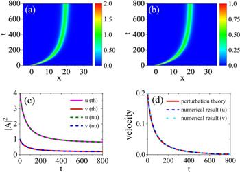
Figure 2. (a) (b) Shown the module evolution of coupled solitons ∣u∣ and ∣v∣, respectively. (c), (d) represent the evolution of amplitude square (∣A∣2) and velocity with time, respectively. The solid lines (th) and dashed lines (nu) denote perturbation theory and numerical result in (c), respectively. We can see the amplitude tends to the fixed point when the velocity to zero. Initial solitons’ states are a1 = 2, a2 = 1, ξ = 0.1, A1 = A2 = 3, B1 = B2 = 1, ε = 0.001. |
3.3. Solitons under different perturbation parameter ratios
We extend our investigation to explore the behavior of bright-bright solitons when $\tfrac{{B}_{1}}{{A}_{1}}\ne \tfrac{{B}_{2}}{{A}_{2}}$. To validate our theoretical predictions, we numerically iterate equation (9 ), (12 ), and (13 ) using the fourth-order Runge–Kutta method, and compare the results with the real-time evolution of the original dynamical equations
Firstly, we aim to investigate a specific scenario where one component has no dissipation while the other one does. To illustrate this case, we set the parameters A2 = B2 = 0 and A1 = 6, B1 = 1. By doing so, we can observe the behavior of solitons under the influence of nonlinear coupling and dissipation in only one component. Figures 3(a) and (b) display the evolution of amplitude and velocity of two-component solitons. Our numerical simulations indicate that ${a}_{1}^{2}+{a}_{2}^{2}=\tfrac{3{B}_{1}}{{A}_{1}}=0.5$, and a soliton attractor is present.
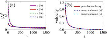
Figure 3. (a), (b) Evolution of two-component amplitude square (∣A∣2) and velocity with A1 = 6, B1 = 1, A2 = B2 = 0. The solid lines (th) and dashed lines (nu) denote perturbation theory and numerical result, respectively. The initial state is a10 = 2, a20 = 1, ξ0 = 0.6, and ε = 0.001. |
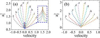
Secondly, we randomly select ten initial states in the form of equations (3 ) and (4 ) with different velocities and amplitudes, while setting the parameter A1 = 6, B1 = 2, and A2 = 9, B2 = 0.75. The evolution of these states in the perturbed system is illustrated in figure 4. Figure 4(a) indicates that the soliton in the u component tends to have an amplitude of ${a}_{1}^{2}=\tfrac{3{B}_{1}}{{A}_{1}}=1$, while the soliton in the v component eventually becomes destroyed, that is, ${a}_{2}^{2}\to 0$ (see figure 4(b)). The soliton’s velocity also tends to be zero as expected. Unlike the ones in figure 1, both components exhibit soliton attractors. We can determine which component’s amplitude tends to zero by utilizing equations (9 ), (12 ), (13 ) in other equation parameters setting.
Figure 4. (a), (b) Represent the evolutions of ten randomly initial coupled solitons (a–j) in ${a}_{1}^{2}$- and ${a}_{2}^{2}$-velocity space. The initial parameters setting for the ten lines are, a1 (a–j): 1.2, 1.3, 1.4, 1.5, 1.6, 1.6, 1.5, 1.4, 1.3, 1.2, a2: 1.1, 1.2, 1.4, 1.6, 1.7, 1.7, 1.6, 1.4, 1.2, 1.1, and the corresponding velocities are vc = 2ξ, vc: −1, −0.8, −0.6, −0.4, −0.2, 0.2, 0.4, 0.6, 0.8, 1. The other parameters are A1 = 6, B1 = 2, A2 = 9, B2 = 0.75, ε = 0.001. |
Based on our numerical simulations, we found that when B1/A1 > B2/A2, the u-component persists while the v-component is destroyed. Conversely, when B1/A1 < B2/A2, the v-component persists while the u-component is destroyed.
4. Conclusion
In this paper, we investigate the behavior of two-component coupling solitons with weak dissipation effects using Lagrangian perturbation analysis. We predict solitonic attractors in $({a}_{1}^{2}+{a}_{2}^{2},{v}_{c})$ space, but there are no fixed points in each component. The final states of the two components depend on the initial conditions, but they can still reach stationary states when the dissipation term ratios are identical for both components. The final amplitudes and velocities can be obtained numerically by solving quasi-particle analysis equations, namely equation (9 ), equation (12 ) and equation (13 ). Explicit expressions for solitonic attractors with identical perturbation ratios are derived, and we describe how coupling solitons evolve with different perturbation ratios. When the dissipation term ratios are different, there are solitonic attractors for both components. It should be noted that the solitonic solutions may become unstable if the condition ∣ε∣ ≪ 1 is not well satisfied [45]. It would be interesting to explore the cases with g ≠ 1, more dissipation effects [39], and high-order effects [46, 47], which may lead to more diverse soliton attractor patterns.