Welcome to visit Communications in Theoretical Physics,
Quantum Physics and Quantum Information

Separability criteria based on a class of symmetric measurements

  • Lemin Lai , 1, 2 ,
  • Shunlong Luo 1, 2
Expand
  • 1Academy of Mathematics and Systems Science, Chinese Academy of Sciences, Beijing 100190, China
  • 2School of Mathematical Sciences, University of Chinese Academy of Sciences, Beijing 100049, China

Received date: 2023-03-12

  Revised date: 2023-04-15

  Accepted date: 2023-04-17

  Online published: 2023-05-24

Copyright

© 2023 Institute of Theoretical Physics CAS, Chinese Physical Society and IOP Publishing

Abstract

Highly symmetric quantum measurements, such as mutually unbiased measurements (MUMs) and general symmetric informationally complete positive-operator-valued measures (GSIC-POVMs), play an important role in both foundational and practical aspects of quantum information theory. Recently, a broad class of symmetric measurements were introduced [K Siudzińska, (2022) Phys. Rev. A 105, 042209], which can be viewed as a common generalization of MUMs and GSIC-POVMs. In this work, the role of these symmetric measurements in entanglement detection is studied. More specifically, based on the correlation matrices defined via (informationally complete) symmetric measurements, a separability criterion for arbitrary dimensional bipartite systems is proposed. It is shown that the criterion is stronger than the method provided by Siudzińska, meanwhile, it can unify several popular separability criteria based on MUMs or GSIC-POVMs. Furthermore, using these (informationally complete) symmetric measurements, two efficient criteria are presented to detect the entanglement of tripartite quantum states. The detection power and advantages of these criteria are illustrated through several examples.

Cite this article

Lemin Lai , Shunlong Luo . Separability criteria based on a class of symmetric measurements[J]. Communications in Theoretical Physics, 2023 , 75(6) : 065101 . DOI: 10.1088/1572-9494/accd5b

1. Introduction

Quantum entanglement is one of the key features of quantum mechanics [13]. As an essential resource, it plays a significant role in many tasks in quantum information and computation, such as quantum cryptography [4], quantum dense coding [5], quantum teleportation [6] and quantum secret sharing [7]. A fundamental issue in the theory of quantum entanglement is to determine whether a given quantum state is entangled or not. The issue is well understood for pure states. However, the situation is extremely complicated for mixed states and there are no general practical criteria until now.
For bipartite quantum systems, a number of criteria to detect entanglement have been proposed from different points of view, such as the positive partial transposition (PPT) criterion [810], the reduction criterion [11], the computable cross-norm or realignment (CCNR) criterion [12, 13], the covariance matrix criterion [1416], the criterion based on Bloch representations [17], the criterion based on local uncertainty relations [1820], and the criterion based on quantum Fisher information [21] etc. See, e.g., [2, 3] for comprehensive surveys. However, for multipartite quantum systems, the detection of entanglement becomes more difficult due to the complexity of multipartite quantum states. There are some separability criteria for multipartite quantum states, which are natural generalizations of those for bipartite cases, for instance, the multipartite reduction criterion [22], the multipartite realignment criterion [23], the multipartite covariance matrix criterion [24], the multipartite criterion based on Bloch representations [25], and the multipartite criterion based on local uncertainty relations [26].
Quantum measurements are important tools in quantum information processing for extracting information from quantum states. Recently, the separability criteria based on quantum measurements are attracting increasing interest, since they are easily implemented in experiments. There are two broadly useful and popular classes of measurements known as mutually unbiased measurements (MUMs) [27] and positive-operator-valued measures (GSIC-POVMs) [28], which are natural extensions of the familiar mutually unbiased bases (MUBs) [2932] and symmetric informationally complete positive-operator-valued measures (SIC-POVMs) [3335], respectively. Moreover, unlike the MUBs and SIC-POVMs, the complete set of MUMs and GSIC-POVMs can be constructed explicitly in all finite dimensions. These measurements are widely applied to the detection of entanglement, and thus a series of efficient separability criteria have been proposed both for bipartite and multipartite systems to date [3645]. It has been shown that the existing criteria based on MUMs and GSIC-POVMs are very powerful in detecting the entanglement of bipartite quantum states, however, how to construct efficient criteria for multipartite quantum states is in general a hard issue. Recently, Siudzińska introduced a broad class of symmetric measurements [46], which includes the MUMs and GSIC-POVMs as special cases. Moreover, possible applications of these symmetric measurements are further discussed in [4648], such as the entropic uncertainty relations and entanglement detection.
In this work, based on the correlation matrices constructed from the (informationally complete) symmetric measurements [46], we first propose a separability criterion for arbitrary dimensional bipartite systems, which is more powerful than the corresponding one in [46]. Interestingly, when choosing MUMs or GSIC-POVMs as local measurements for two subsystems, it reproduces several criteria known before. Employing these symmetric measurements, we further derive two effective separability criteria in terms of tripartite correlation matrices.
The work is arranged as follows. In section 2, we review the notion of symmetric measurements and their main features. In section 3, we derive several separability criteria based on (informationally complete) symmetric measurements for bipartite and tripartite systems, respectively. We further illustrate the effectiveness of our method through several examples in section 4. Finally, we conclude with a summary in section 5. Detailed proofs of the main results (theorems 13) are relegated to the appendix.

2. Symmetric measurements

In [46], a broad class of symmetric measurements were introduced. Here we recall the definition and main properties.
A collection {Sμ: μ = 1, 2, …, s} consisting of s POVMs Sμ = {Sμ,i: i = 1, 2, …, t} on ${{\mathbb{C}}}^{d}$ is called a set of symmetric measurements if
i

(i) $\mathrm{tr}({S}_{\mu ,i})=\tfrac{d}{t}$,

ii

(ii) $\mathrm{tr}({S}_{\mu ,i}^{2})=\chi ,$

iii

(iii) $\mathrm{tr}({S}_{\mu ,i}{S}_{\mu ,j})=\tfrac{d-t\chi }{t(t-1)},\quad i\ne j$,

iv

(iv) $\mathrm{tr}({S}_{\mu ,i}{S}_{\nu ,j})=\tfrac{d}{{t}^{2}},\quad \mu \ne \nu $

with a free parameter χ satisfying
$\begin{eqnarray}\displaystyle \frac{d}{{t}^{2}}\lt \chi \leqslant \min \left\{\displaystyle \frac{{d}^{2}}{{t}^{2}},\displaystyle \frac{d}{t}\right\}.\end{eqnarray}$
The set ${ \mathcal S }(s,t)=\{{S}_{\mu ,i}:\mu =1,2,\,\ldots ,\,s;i\,=\,1,2,\,\ldots ,\,t\}$ is called an (s, t)-POVM [46]. If χ = d2/t2, then the constituent POVMs are projective measurements (td). This notion encapsulates several important and special instances:
1.

(1)a complete set of MUBs for s = d + 1, t = d and χ = 1,

2.

(2)an equiangular tight frame for s = 1, χ = d2/t2, t ∈ {d, d + 1, …, d2}[49, 50],

3.

(3)an SIC-POVM for s = 1, t = d2 and χ = 1/d2.

The set ${ \mathcal S }(s,t)$ is informationally complete if and only if
$\begin{eqnarray}s=\displaystyle \frac{{d}^{2}-1}{t-1}.\end{eqnarray}$
It has been shown that for any finite dimension d (d > 2), there exist at least four informationally complete (s, t)-POVMs depending on the choice of s and t:
1.

(1)s = 1 and t = d2 (GSIC-POVMs),

2.

(2)s = d + 1 and t = d (MUMs),

3.

(3)s = d2 − 1 and t = 2,

4.

(4)s = d − 1 and t = d + 2.

For the case d = 2, there are only two possible choices of the parameters s and t: s = 1, t = 4 (GSIC-POVMs) and s = 3, t = 2 (MUMs), which provide a unified method to describe GSIC-POVMs and MUMs.
In [46], a general construction of informationally complete (s, t)-POVMs for arbitrary dimensions has been presented by an orthonormal Hermitian operator basis. Let {Hμ,i: μ = 1, 2, …, s; i = 1, 2, …, t − 1} be a set of (st − 1) Hermitian and traceless operators on ${{\mathbb{C}}}^{d}$ satisfying $\mathrm{tr}({H}_{\mu ,i}{H}_{{\mu }^{{\prime} },{i}^{{\prime} }})={\delta }_{\mu {\mu }^{{\prime} }}{\delta }_{{{ii}}^{{\prime} }},$ then the operators
$\begin{eqnarray}{S}_{\mu ,i}=\displaystyle \frac{1}{t}{{\bf{1}}}_{d}+{{rR}}_{\mu ,i},\quad \mu =1,2,\quad \cdots ,\quad s;i=1,2,\quad \cdots ,\quad t\end{eqnarray}$
form an informationally complete (s, t)-POVM. Here
$\begin{eqnarray}{R}_{\mu ,i}=\left\{\begin{array}{ll}{H}_{\mu }-\sqrt{t}(\sqrt{t}+1){H}_{\mu ,i}, & i=1,2,\,\ldots ,\,t-1,\\ (\sqrt{t}+1){H}_{\mu }, & i=t,\end{array}\right.\end{eqnarray}$
and ${H}_{\mu }={\sum }_{i=1}^{t-1}{H}_{\mu ,i}.$ The parameter r should be chosen such that Sμ,i ≥ 0, which implies that
$\begin{eqnarray*}-\displaystyle \frac{1}{t{\lambda }_{\max }}\leqslant r\leqslant \displaystyle \frac{1}{t| {\lambda }_{\min }| },\end{eqnarray*}$
where ${\lambda }_{\max }$ and ${\lambda }_{\min }$ are the maximum and minimum eigenvalues among all eigenvalues of the operators Rμ,i, respectively. The parameter χ is related to r and t via
$\begin{eqnarray}\chi =\displaystyle \frac{d}{{t}^{2}}+{r}^{2}(t-1){\left(\sqrt{t}+1\right)}^{2},\end{eqnarray}$
and the maximum value ${\chi }_{\max }$ is obtained when
$\begin{eqnarray*}r=\max \left\{\displaystyle \frac{1}{t{\lambda }_{\max }},\displaystyle \frac{1}{t| {\lambda }_{\min }| }\right\}.\end{eqnarray*}$
For instance, when d = 3, we can construct four informationally complete (s, t)-POVMs from the generalized Gell-Mann (GM) operator basis [51]. We list the range of the parameter r and the maximum value ${\chi }_{\max }$ in table 1.
Table 1. The range of the parameter r and the maximum value ${\chi }_{\max }$ for the four informationally complete (s, t)-POVMs on ${{\mathbb{C}}}^{3}$. These measurements are constructed from the generalized GM operators.
(s, t)-POVM r ${\chi }_{\max }$
(1, 9) −0.0121 ≤ r ≤ 0.0129 0.0583
(4, 3) −0.1093 ≤ r ≤ 0.1220 0.5555
(8, 2) −0.2536 ≤ r ≤ 0.2536 0.1250
(2, 5) −0.0383 ≤ r ≤ 0.0388 0.1831
Let {Sμ,i: μ = 1, 2, …, s; i = 1, 2, …, t} be any informationally complete (s, t)-POVM on ${{\mathbb{C}}}^{d}$. It has been shown that for any state ρ on ${{\mathbb{C}}}^{d}$, it holds that [46]
$\begin{eqnarray}\sum _{\mu =1}^{s}\sum _{i=1}^{t}{\left(\mathrm{tr}({S}_{\mu ,i}\rho )\right)}^{2}=\displaystyle \frac{d({t}^{2}\chi -d)\mathrm{tr}({\rho }^{2})+{d}^{3}-{t}^{2}\chi }{{dt}(t-1)}\end{eqnarray}$
$\begin{eqnarray}\leqslant \,\displaystyle \frac{(d-1)({d}^{2}+{t}^{2}\chi )}{{dt}(t-1)},\end{eqnarray}$
where the equality holds when ρ is a pure state.

3. Detecting entanglement via symmetric measurements

In this section, based on the (informationally complete) symmetric measurements, we present some separability criteria for arbitrary dimensional bipartite and tripartite systems, respectively.

3.1. Separability criteria for bipartite systems

Let $\mathcal{S}^a=\{S_{\mu,m}^a;\mu=1,2,...,s_a;m=1,2,...,t_a\}$ and $\mathcal{S}^b=\left\{S_{\nu, n}^b: \nu=1,2, \ldots, s_b ; n=1,2, \ldots, t_b\right\}$ be two sets of informationally complete, symmetric measurements on ${{\mathbb{C}}}^{{d}_{a}}$ and ${{\mathbb{C}}}^{{d}_{b}}$ with parameters χa and χb, respectively. For a given state ρ on ${{\mathbb{C}}}^{{d}_{a}}\otimes {{\mathbb{C}}}^{{d}_{b}}$, the correlation matrix associated with these data is defined as
$\begin{eqnarray}C(\rho | {{ \mathcal S }}^{a},{{ \mathcal S }}^{b})=\left(\Space{0ex}{1ex}{0ex}\mathrm{tr}\left(({S}_{i}^{a}\otimes {S}_{j}^{b})(\rho -{\rho }_{a}\times {\rho }_{b})\right)\Space{0ex}{1ex}{0ex}\right),\end{eqnarray}$
for i = 1, 2, …, sata, j = 1, 2, …, sbtb, where
$\begin{eqnarray}\begin{array}{ll}{S}_{i}^{a}={S}_{\mu ,m}^{a}, & i=(\mu -1){t}_{a}+m,\\ & \mu =1,2,\,\ldots ,\,{s}_{a},m=1,2,\,\ldots ,\,{t}_{a},\end{array}\end{eqnarray}$
$\begin{eqnarray}\begin{array}{ll}{S}_{j}^{b}={S}_{\nu ,n}^{b}, & j=(\nu -1){t}_{b}+n,\\ & \nu =1,2,\,\ldots ,\,{s}_{b},n=1,2,\,\ldots ,\,{t}_{b},\end{array}\end{eqnarray}$
and ${\rho }_{a}={\mathrm{tr}}_{b}\rho $, ${\rho }_{b}={\mathrm{tr}}_{a}\rho $ are reduced states. Next we establish a separability criterion in terms of the above correlation matrix.

With the above notation, if ρ is separable, then

$\begin{eqnarray}\parallel C(\rho | {{ \mathcal S }}^{a},{{ \mathcal S }}^{b}){\parallel }_{\mathrm{tr}}\leqslant \sqrt{{\upsilon }_{a}(1-\mathrm{tr}({\rho }_{a}^{2})){\upsilon }_{b}(1-\mathrm{tr}({\rho }_{b}^{2}))},\end{eqnarray}$
where $\parallel \cdot {\parallel }_{\mathrm{tr}}$ stands for the trace norm (i.e., the sum of singular values of a matrix), and
$\begin{eqnarray}{\upsilon }_{a}=\displaystyle \frac{{t}_{a}^{2}{\chi }_{a}-{d}_{a}}{{t}_{a}({t}_{a}-1)},\qquad {\upsilon }_{b}=\displaystyle \frac{{t}_{b}^{2}{\chi }_{b}-{d}_{b}}{{t}_{b}({t}_{b}-1)}.\end{eqnarray}$

A Space for the proof, see the appendix.
If we define the matrix
$\begin{eqnarray*}D(\rho | {{ \mathcal S }}^{a},{{ \mathcal S }}^{b})=\left(\Space{0ex}{1ex}{0ex}\mathrm{tr}\left(({S}_{i}^{a}\otimes {S}_{j}^{b})\rho \right)\Space{0ex}{1ex}{0ex}\right),\end{eqnarray*}$
then the separability criterion in [46] states that any separable state ρ on ${{\mathbb{C}}}^{{d}_{a}}\otimes {{\mathbb{C}}}^{{d}_{b}}$ must satisfy
$\begin{eqnarray}\parallel D(\rho | {{ \mathcal S }}^{a},{{ \mathcal S }}^{b}){\parallel }_{\mathrm{tr}}\leqslant \sqrt{{\widetilde{\upsilon }}_{a}{\widetilde{\upsilon }}_{b}},\end{eqnarray}$
with
$\begin{eqnarray}{\widetilde{\upsilon }}_{a}=\displaystyle \frac{({d}_{a}-1)({d}_{a}^{2}+{t}_{a}^{2}{\chi }_{a})}{{d}_{a}{t}_{a}({t}_{a}-1)},{\widetilde{\upsilon }}_{b}=\displaystyle \frac{({d}_{b}-1)({d}_{b}^{2}+{t}_{b}^{2}{\chi }_{b})}{{d}_{b}{t}_{b}({t}_{b}-1)}.\end{eqnarray}$
Now we show that, for the same symmetric measurements, the separability criterion in theorem 1 is more efficient than the criterion determined by inequality (13).
Let
$\begin{eqnarray*}{\boldsymbol{\alpha }}=\left(\begin{array}{c}{\alpha }_{1}\\ {\alpha }_{2}\\ \vdots \\ {\alpha }_{{s}_{a}{t}_{a}}\end{array}\right),\qquad {\boldsymbol{\beta }}=\left(\begin{array}{c}{\beta }_{1}\\ {\beta }_{2}\\ \vdots \\ {\beta }_{{s}_{b}{t}_{b}}\end{array}\right)\end{eqnarray*}$
with
$\begin{eqnarray*}\begin{array}{rcl}{\alpha }_{i} & = & \mathrm{tr}({S}_{i}^{a}{\rho }_{a}),\qquad i=1,2,\,\ldots ,\,{s}_{a}{t}_{a},\\ {\beta }_{j} & = & \mathrm{tr}({S}_{j}^{b}{\rho }_{b}),\qquad j=1,2,\,\ldots ,\,{s}_{b}{t}_{b},\end{array}\end{eqnarray*}$
then $C(\rho | {{ \mathcal S }}^{a},{{ \mathcal S }}^{b})=D(\rho | {{ \mathcal S }}^{a},{{ \mathcal S }}^{b})-{\boldsymbol{\alpha }}{{\boldsymbol{\beta }}}^{{\rm{T}}}$ (T stands for the transpose). Assuming that inequality (11) holds, then
$\begin{eqnarray*}\begin{array}{l}\parallel D(\rho | {{ \mathcal S }}^{a},{{ \mathcal S }}^{b}){\parallel }_{\mathrm{tr}}\\ \,\leqslant \parallel C(\rho | {{ \mathcal S }}^{a},{{ \mathcal S }}^{b}){\parallel }_{\mathrm{tr}}+\parallel {\boldsymbol{\alpha }}{{\boldsymbol{\beta }}}^{{\rm{T}}}{\parallel }_{\mathrm{tr}}\\ \,\leqslant \sqrt{{\upsilon }_{a}(1-\mathrm{tr}({\rho }_{a}^{2})){\upsilon }_{b}(1-\mathrm{tr}({\rho }_{b}^{2}))}+\parallel {\boldsymbol{\alpha }}\parallel \parallel {\boldsymbol{\beta }}\parallel \\ =\sqrt{{\widetilde{\upsilon }}_{a}-\sum _{i=1}^{{s}_{a}{t}_{a}}{\left(\mathrm{tr}{S}_{i}^{a}{\rho }_{a}\right)}^{2}}\sqrt{{\widetilde{\upsilon }}_{b}-\sum _{j=1}^{{s}_{b}{t}_{b}}{\left(\mathrm{tr}{S}_{j}^{b}{\rho }_{b}\right)}^{2}}\\ \qquad +\parallel {\boldsymbol{\alpha }}\parallel \parallel {\boldsymbol{\beta }}\parallel \\ =\sqrt{{\widetilde{\upsilon }}_{a}-\sum _{i=1}^{{s}_{a}{t}_{a}}{\left(\mathrm{tr}{S}_{i}^{a}{\rho }_{a}\right)}^{2}}\sqrt{{\widetilde{\upsilon }}_{b}-\sum _{j=1}^{{s}_{b}{t}_{b}}{\left(\mathrm{tr}{S}_{j}^{b}{\rho }_{b}\right)}^{2}}\\ \qquad +\sqrt{\sum _{i=1}^{{s}_{a}{t}_{a}}{\left(\mathrm{tr}{S}_{i}^{a}{\rho }_{a}\right)}^{2}}\sqrt{\sum _{j=1}^{{s}_{b}{t}_{b}}{\left(\mathrm{tr}{S}_{j}^{b}{\rho }_{b}\right)}^{2}}\\ \,\leqslant \sqrt{{\widetilde{\upsilon }}_{a}\widetilde{{\upsilon }_{b}}},\end{array}\end{eqnarray*}$
where ∥ · ∥ denotes the Euclidean norm of vectors and the third inequality is due to $\sqrt{c}\sqrt{d}+\sqrt{e}\sqrt{f}\leqslant \sqrt{c+e}\sqrt{d+f}$ for any non-negative c, d, e, f.
Consider the simplest case da = db = d, sa = sb = s, ta = tb = t and χa = χb = χ, then from inequalities (11) and (13) we conclude that any separable state ρ satisfies
$\begin{eqnarray}\begin{array}{l}\sum _{\mu =1}^{s}\sum _{i=1}^{t}\left|\mathrm{tr}\left(({S}_{\mu ,i}^{a}\otimes {S}_{\mu ,i}^{b})(\rho -{\rho }_{a}\otimes {\rho }_{b})\right)\right|\\ \,\leqslant \displaystyle \frac{{t}^{2}\chi -d}{t(t-1)}\sqrt{(1-\mathrm{tr}({\rho }_{a}^{2}))(1-\mathrm{tr}({\rho }_{b}^{2}))},\end{array}\end{eqnarray}$
and
$\begin{eqnarray}\sum _{\mu =1}^{s}\sum _{i=1}^{t}\mathrm{tr}\left(({S}_{\mu ,i}^{a}\otimes {S}_{\mu ,i}^{b})\rho \right)\leqslant \displaystyle \frac{(d-1)({d}^{2}+{t}^{2}\chi )}{{dt}(t-1)},\end{eqnarray}$
by the inequality ${\sum }_{i=1}^{k}| {c}_{{ii}}| \leqslant \parallel C{\parallel }_{\mathrm{tr}}$ for any matrix $C\,=({c}_{{ij}})\in {{\mathbb{C}}}^{k\times k}$.
Interestingly, if we choose MUMs or GSIC-POVMs as local measurements for the two subsystems, respectively, then the separability criteria determined by equations (11), (13), (15) and (16) can recover the ones in [3642], as summarized in table 2.
Table 2. Relations between the separability criteria determined by equations (11), (13), (15) and (16) and the criteria based on GSIC-POVMs (SIC-POVMs) or MUMs (MUBs) in [3642].
GSIC-POVMs (SICs) MUMs (MUBs)
Equation (11) [42] [42]
Equation (13) [41] ([40])
Equation (15) [39] [39]
Equation (16) [38] [37] ([36])

3.2. Separability criteria for tripartite systems

Given a tripartite state ρ on ${{\mathbb{C}}}^{{d}_{a}}\otimes {{\mathbb{C}}}^{{d}_{b}}\otimes {{\mathbb{C}}}^{{d}_{c}}$, consider the informationally complete, symmetric measurements ${{ \mathcal S }}^{a}=\{{S}_{\mu ,m}^{a}:\mu =1,2,\,\ldots ,\,{s}_{a};m=1,2,\,\ldots ,\,{t}_{a}\}$ with the parameter χa, ${{ \mathcal S }}^{b}=\{{S}_{\nu ,n}^{b}:\nu =1,2,\,\ldots ,\,{s}_{b};n=1,2,\,\ldots ,\,{t}_{b}\}$ with the parameter χb, and ${{ \mathcal S }}^{c}=\{{S}_{\omega ,l}^{c}:\omega =1,2,\,\ldots ,\,{s}_{c};l=1,2,\,\ldots ,{t}_{c}\}$ with the parameter χc for the subsystems a, b and c, respectively. Let
$\begin{eqnarray*}{c}_{{ijk}}=\mathrm{tr}\left(({S}_{i}^{a}\otimes {S}_{j}^{b}\otimes {S}_{k}^{c})\rho \right)\end{eqnarray*}$
for i = 1, 2, …, sata, j = 1, 2, …, sbtb and k = 1, 2, …, sctc, where Sai, Sbj are defined by equations (9) and (10), and
$\begin{eqnarray}{S}_{k}^{c}={S}_{\omega ,l}^{c}\end{eqnarray}$
with k = (&ohgr; − 1)tc + l, &ohgr; = 1, 2, …, sc, l = 1, 2, …, tc. We further define three correlation matrices ${E}^{\underline{a}{bc}}$, ${E}^{a\underline{b}c}$ and ${E}^{{ab}\underline{c}}$ among ${{ \mathcal S }}^{a}$, ${{ \mathcal S }}^{b}$ and ${{ \mathcal S }}^{c}$ by
$\begin{eqnarray}{E}^{\underline{a}{bc}}(\rho | {{ \mathcal S }}^{a},{{ \mathcal S }}^{b},{{ \mathcal S }}^{c})={E}^{(1)}\oplus {E}^{(2)}\oplus \cdots \oplus \,{E}^{({s}_{a}{t}_{a})},\end{eqnarray}$
with ${E}^{(i)}=\left({e}_{{jk}}^{(i)}\right)$ and ${e}_{{jk}}^{(i)}={c}_{{ijk}}$ for i = 1, 2, …, sata,
$\begin{eqnarray}{E}^{a\underline{b}c}(\rho | {{ \mathcal S }}^{a},{{ \mathcal S }}^{b},{{ \mathcal S }}^{c})={\widetilde{E}}^{(1)}\oplus {\widetilde{E}}^{(2)}\oplus \cdots \oplus \,{\widetilde{E}}^{({s}_{b}{t}_{b})},\end{eqnarray}$
with ${\widetilde{E}}^{(j)}=\left({\tilde{e}}_{{ik}}^{(j)}\right)$ and ${\tilde{e}}_{{ik}}^{(j)}={c}_{{ijk}}$ for j = 1, 2, …, sbtb,
$\begin{eqnarray}{E}^{{ab}\underline{c}}(\rho | {{ \mathcal S }}^{a},{{ \mathcal S }}^{b},{{ \mathcal S }}^{c})={\hat{E}}^{(1)}\oplus {\hat{E}}^{(2)}\oplus \cdots \oplus \,{\hat{E}}^{({s}_{c}{t}_{c})},\end{eqnarray}$
with ${\hat{E}}^{(k)}=\left({\hat{e}}_{{ij}}^{(k)}\right)$ and ${\hat{e}}_{{ij}}^{(k)}={c}_{{ijk}}$ for k = 1, 2, …, sctc.

With the above data, if a tripartite state ρ on ${{\mathbb{C}}}^{{d}_{a}}\otimes {{\mathbb{C}}}^{{d}_{b}}\otimes {{\mathbb{C}}}^{{d}_{c}}$ is fully separable, then

$\begin{eqnarray}{E}^{\underline{a}{bc}}(\rho | {{ \mathcal S }}^{a},{{ \mathcal S }}^{b},{{ \mathcal S }}^{c})\leqslant {s}_{a}\sqrt{{\widetilde{\upsilon }}_{b}{\widetilde{\upsilon }}_{c}},\end{eqnarray}$
$\begin{eqnarray}{E}^{a\underline{b}c}(\rho | {{ \mathcal S }}^{a},{{ \mathcal S }}^{b},{{ \mathcal S }}^{c})\leqslant {s}_{b}\sqrt{{\widetilde{\upsilon }}_{a}{\widetilde{\upsilon }}_{c}},\end{eqnarray}$
$\begin{eqnarray}{E}^{{ab}\underline{c}}(\rho | {{ \mathcal S }}^{a},{{ \mathcal S }}^{b},{{ \mathcal S }}^{c})\leqslant {s}_{c}\sqrt{{\widetilde{\upsilon }}_{a}{\widetilde{\upsilon }}_{b}},\end{eqnarray}$
where ${\widetilde{\upsilon }}_{a}$ and ${\widetilde{\upsilon }}_{b}$ are defined by equation (14), and
$\begin{eqnarray}{\widetilde{\upsilon }}_{c}=\displaystyle \frac{({d}_{c}-1)({d}_{c}^{2}+{t}_{c}^{2}{\chi }_{c})}{{d}_{c}{t}_{c}({t}_{c}-1)}.\end{eqnarray}$

For the proof, see the appendix.
We can extend the bipartite separability criterion determined by equation (13) to the tripartite case: define three correlation matrices ${G}^{\underline{a}{bc}}$,${G}^{a\underline{b}c}$ and ${G}^{{ab}\underline{c}}$ among ${{ \mathcal S }}^{a}$, ${{ \mathcal S }}^{b}$ and ${{ \mathcal S }}^{c}$ by
$\begin{eqnarray}{G}^{\underline{a}{bc}}(\rho | {{ \mathcal S }}^{a},{{ \mathcal S }}^{b},{{ \mathcal S }}^{c})=\left(\Space{0ex}{1ex}{0ex}~{g}_{i,{s}_{c}~{t}_{c}~(j-1)~+k}~\Space{0ex}{1.6ex}{0ex}\right),\end{eqnarray}$
with ${g}_{i,~{s}_{c}~{t}_{c}~(j-1)+k}~=~{c}_{{~i~j~k}}$,
$\begin{eqnarray}{G}^{a\underline{b}c}(\rho | {{ \mathcal S }}^{a},{{ \mathcal S }}^{b},{{ \mathcal S }}^{c})=\left(\Space{0ex}{1ex}{0ex}~{\tilde{g}}_{j,~{s}_{c}~{t}_{c}~(i-1)+k}\Space{0ex}{1ex}{0ex}~\right),\end{eqnarray}$
with ${\tilde{g}}_{j,~{s}_{c}~{t}_{c}~(i-1)+k}~=~{c}_{{i~j~k}}$,
$\begin{eqnarray}{G}^{{ab}\underline{c}}(\rho | {{ \mathcal S }}^{a},{{ \mathcal S }}^{b},{{ \mathcal S }}^{c})=\left(\Space{0ex}{1ex}{0ex}~{\hat{g}}_{k,~{s}_{b}~{t}_{b}~(i-1)+j}~\Space{0ex}{1ex}{0ex}\right),\end{eqnarray}$
with ${\hat{g}}_{k,~{s}_{b}~{t}_{b}~(i-1)+j}~=~{c}_{{i~j~k}}$.
In the following, we present another tripartite separability criterion based on the above correlation matrix.

If a tripartite state ρ on ${{\mathbb{C}}}^{{d}_{a}}\otimes {{\mathbb{C}}}^{{d}_{b}}\otimes {{\mathbb{C}}}^{{d}_{c}}$ is fully separable, then

$\begin{eqnarray}{G}^{\underline{a}{bc}}(\rho | {{ \mathcal S }}^{a},{{ \mathcal S }}^{b},{{ \mathcal S }}^{c})\leqslant \sqrt{{\widetilde{\upsilon }}_{a}{\widetilde{\upsilon }}_{b}{\widetilde{\upsilon }}_{c}},\end{eqnarray}$
$\begin{eqnarray}{G}^{a\underline{b}c}(\rho | {{ \mathcal S }}^{a},{{ \mathcal S }}^{b},{{ \mathcal S }}^{c})\leqslant \sqrt{{\widetilde{\upsilon }}_{a}{\widetilde{\upsilon }}_{b}{\widetilde{\upsilon }}_{c}},\end{eqnarray}$
$\begin{eqnarray}{G}^{{ab}\underline{c}}(\rho | {{ \mathcal S }}^{a},{{ \mathcal S }}^{b},{{ \mathcal S }}^{c})\leqslant \sqrt{{\widetilde{\upsilon }}_{a}{\widetilde{\upsilon }}_{b}{\widetilde{\upsilon }}_{c}},\end{eqnarray}$
where ${\widetilde{\upsilon }}_{a}$, ${\widetilde{\upsilon }}_{b}$ and ${\widetilde{\upsilon }}_{c}$ is given as in theorem 2. For the proof, see the appendix.

4. Illustration

In what follows, we provide some examples to illustrate the efficiency of the criteria in theorems 13.
Example 1. Consider the d × d-dimensional isotropic states
$\begin{eqnarray}{\rho }_{\mathrm{iso}}(p)=\displaystyle \frac{1-p}{{d}^{2}}{{\bf{1}}}_{{d}^{2}}+p| {\psi }_{d}^{+}\rangle \langle {\psi }_{d}^{+}| ,\qquad 0\leqslant p\leqslant 1,\end{eqnarray}$
where $| {\psi }_{d}^{+}\rangle ={\sum }_{i=0}^{d-1}| {ii}\rangle /\sqrt{d}$. The isotropic states ρiso(p) are entangled if and only if p > 1/(d + 1) [11].
Let ${ \mathcal S }=\{{S}_{\mu ,m}:\mu =1,2,\,\ldots ,\,s;m=1\,2,\,\ldots ,\,t\}$ be a set of informationally complete, symmetric measurements on ${{\mathbb{C}}}^{d}$ with parameter χ, then the complex conjugate (relative to the computational basis of ${{\mathbb{C}}}^{d}$) ${{ \mathcal S }}^{* }=\{{S}_{\mu ,m}^{* }:\mu =1,2,\,\ldots ,\,s;m=1,2,\,\ldots ,\,t\}$ also is a set of informationally complete, symmetric measurements on ${{\mathbb{C}}}^{d}.$ We use them to detect the separability of ρiso(p).
After simple computations, we get the correlation matrix
$\begin{eqnarray*}C({\rho }_{\mathrm{iso}}(p)| { \mathcal S },{{ \mathcal S }}^{* })=Z\oplus Z\oplus \cdots \oplus \,Z,\end{eqnarray*}$
where the number of summands is s, and Z = (zij) is a t × t matrix with the entries
$\begin{eqnarray*}{z}_{{ij}}=\left\{\begin{array}{ll}\tfrac{p({t}^{2}\chi -d)}{{{dt}}^{2}}, & i=j\\ \tfrac{p(d-{t}^{2}\chi )}{{{dt}}^{2}(t-1)}, & i\ne j.\end{array}\right.\end{eqnarray*}$
Consequently, the matrix Z is real and non-negative definite, which has the spectrum
$\begin{eqnarray*}\displaystyle \frac{p({t}^{2}\chi -d)}{{dt}(t-1)}\left\{1,1,\cdots ,1,0\right\}.\end{eqnarray*}$
Hence,
$\begin{eqnarray*}\begin{array}{rcl}\parallel C({\rho }_{\mathrm{iso}}(p))| { \mathcal S },{{ \mathcal S }}^{* }{\parallel }_{\mathrm{tr}} & = & s(t-1)\displaystyle \frac{p({t}^{2}\chi -d)}{{dt}(t-1)}\\ & = & \displaystyle \frac{{ps}({t}^{2}\chi -d)}{{dt}}.\end{array}\end{eqnarray*}$
Moreover, we have $\mathrm{tr}({\rho }_{a}^{2})=\mathrm{tr}({\rho }_{b}^{2})=1/d$. Employing theorem 1, we conclude that ρiso(p) are entangled for p > 1/(d + 1). Thus theorem 1 can detect all the entanglement of the isotropic states for any dimension d.
Example 2. Consider the d-dimensional Werner states [52]
$\begin{eqnarray}{\rho }_{{\rm{w}}}(f)=\displaystyle \frac{d-f}{{d}^{3}-d}{{\bf{1}}}_{{d}^{2}}+\displaystyle \frac{{df}-1}{{d}^{3}-d}V,\qquad -1\leqslant f\leqslant 1,\end{eqnarray}$
where $V={\sum }_{i,j=0}^{d-1}| {ij}\rangle \langle {ji}| $. It has been shown that ρw(f) are entangled if and only if −1 ≤ f ≤ 0. Let ${ \mathcal S }=\{{S}_{\mu ,m}:\mu =1,2,\,\ldots ,\,s;m=1,2,\,\ldots ,\,t\}$ be a set of informationally complete, symmetric measurements on ${{\mathbb{C}}}^{d}$ with parameter χ. By direct calculation, we have
$\begin{eqnarray*}\parallel C({\rho }_{{\rm{w}}}(f)| { \mathcal S },{ \mathcal S }){\parallel }_{\mathrm{tr}}=\displaystyle \frac{s| {df}-1| ({t}^{2}\chi -d)}{t({d}^{3}-d)},\end{eqnarray*}$
which, via inequality (11), implies that ρw(f) are entangled for $-1\leqslant f\lt \tfrac{2}{d}-1$. Thus theorem 1 can recognize the entanglement of ρw(f) for $-1\leqslant f\lt \tfrac{2}{d}-1$, which coincides with the result in [39].
Example 3. Consider the family of 3 × 3 states
$\begin{eqnarray}\rho (\tau ,q)=q\rho (\tau )+(1-q)\displaystyle \frac{{{\bf{1}}}_{9}}{9},\end{eqnarray}$
where 0 < τ < 1 and 0 ≤ q ≤ 1,
$\begin{eqnarray*}\rho (\tau )=\displaystyle \frac{1}{8\tau +1}\left(\begin{array}{ccccccccc}\tau & 0 & 0 & 0 & \tau & 0 & 0 & 0 & \tau \\ 0 & \tau & 0 & 0 & 0 & 0 & 0 & 0 & 0\\ 0 & 0 & \tau & 0 & 0 & 0 & 0 & 0 & 0\\ 0 & 0 & 0 & \tau & 0 & 0 & 0 & 0 & 0\\ \tau & 0 & 0 & 0 & \tau & 0 & 0 & 0 & \tau \\ 0 & 0 & 0 & 0 & 0 & \tau & 0 & 0 & 0\\ 0 & 0 & 0 & 0 & 0 & 0 & \tfrac{1+\tau }{2} & 0 & \tfrac{\sqrt{1-{\tau }^{2}}}{2}\\ 0 & 0 & 0 & 0 & 0 & 0 & 0 & \tau & 0\\ \tau & 0 & 0 & 0 & \tau & 0 & \tfrac{\sqrt{1-{\tau }^{2}}}{2} & 0 & \tfrac{1+\tau }{2}\end{array}\right)\end{eqnarray*}$
is a 3 × 3 bound entangled state given by Horodecki [10].
We have shown that inequality (11) is stronger than inequality (13). Now we specifically compare the detection power of these two criteria using the informationally complete (8, 2)-POVM, which is constructed from the generalized GM matrices with the parameter χ = 0.125. In figure 1, we illustrate the ranges of the parameters q and τ for which the entanglement of ρ(τ, p) is detected by inequalities (11) and (13), respectively. It is clear that theorem 1 can detect more entangled states than that in [46] for the same measurement settings.
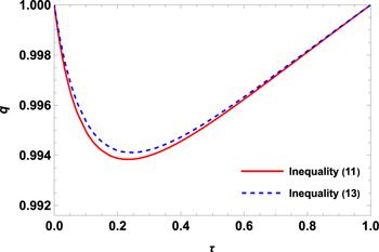
Figure 1. Comparison of the detection power between inequalities (11) and (13) for ρ(τ, q). The red solid and blue dashed lines demarcate the lower borders of the parameter regions for entanglement detected by inequality (11) and inequality (13), respectively. We see that our method can certify more entangled states than inequality (13).
Example 4. Consider the 3 × 3 states given by
$\begin{eqnarray}\rho (h)=\displaystyle \frac{1}{7}| {\psi }_{3}^{+}\rangle \langle {\psi }_{3}^{+}| +\displaystyle \frac{h}{7}{\rho }_{1}+\displaystyle \frac{6-h}{7}{\rho }_{2},\qquad 0\leqslant h\leqslant 1,\end{eqnarray}$
where
$\begin{eqnarray*}\begin{array}{rcl}| {\psi }_{3}^{+}\rangle & = & \displaystyle \frac{| 00\rangle +| 11\rangle +| 22\rangle }{\sqrt{3}},\\ {\rho }_{1} & = & \displaystyle \frac{| 02\rangle \langle 02| +| 10\rangle \langle 10| +| 21\rangle \langle 21| }{3},\\ {\rho }_{2} & = & \displaystyle \frac{| 01\rangle \langle 01| +| 12\rangle \langle 12| +| 20\rangle \langle 20| }{3}.\end{array}\end{eqnarray*}$
From PPT criterion [8], ρ(h) are entangled for 0 ≤ h < 0.1716 and 5.8284 < h ≤ 6. Now employing theorem 1 with (2, 5)-POVM (the parameter χ = 0.1831), we get ρ(h) are entangled for 0 ≤ h < 1 and 5 < h ≤ 6. Moreover, we find that the same entangled conditions can be obtained with (4, 3)-POVM (MUMs with χ = 0.5555) and (1, 9)-POVM (GSIC-POVMs with χ = 0.0583) for these states. Therefore, in this case, the detection power of theorem 1 with three different symmetric measurements coincides and is more powerful than the PPT criterion.
Example 5. Consider the three-qubit state $W=(| 100\rangle +| 010\rangle +| 001\rangle )/\sqrt{3}$ mixed with the identity operator [53]
$\begin{eqnarray}\rho (x)=\displaystyle \frac{x}{8}{{\bf{1}}}_{8}+(1-x)| {\rm{W}}\rangle \langle {\rm{W}}| ,\qquad 0\leqslant x\leqslant 1.\end{eqnarray}$
It has been shown that ρ(x) are entangled for 0 ≤ x < 0.566 from the local uncertainty relation criterion in [26]. Now employing theorem 2 with three MUMs (i.e., s = 3, t = 2), we conclude that ρ(x) are entangled for 0 ≤ x < 4/7 ≈ 0.5714. In a similar way, theorem 2 with GSIC-POVMs (i.e., s = 1, t = 4) can also identify the entanglement of ρ(x) for 0 ≤ x < 4/7. Numerical computations show that the criterion in [44] based on MUMs cannot detect entanglement of ρ(x). Thus, our method in theorem 2 is more powerful than the criterion based on local uncertainty relations, and that in [44] for these states.
Example 6. Consider the three-qutrit states
$\begin{eqnarray}\rho (y)=\displaystyle \frac{1-y}{27}{{\bf{1}}}_{27}+y| {\rm{\Phi }}\rangle \langle {\rm{\Phi }}| ,\qquad 0\leqslant y\leqslant 1\end{eqnarray}$
with ∣Φ⟩ = $\tfrac{1}{\sqrt{6}}(| 002\rangle $ + ∣020⟩ + ∣200⟩ + ∣112⟩ + ∣121⟩ + ∣211⟩).
Now we compare the detection power between theorems 2 and 3. Using theorem 2 with GSIC-POVMs, we conclude that ρ(y) are entangled for 0.3208 ≤ y ≤ 1. Moreover, theorem 3 can detect the entanglement of ρ(y) for 0.3902 ≤ y ≤ 1. Thus theorems 2 and 3 are efficient in detecting the entanglement for certain multipartite systems, and theorem 2 is more efficient than theorem 3 in this case.

5. Summary

In this paper, a class of symmetric measurements introduced in [46], which include MUMs and GSIC-POVMs as special cases, have been used to study the problem of quantum separability. Based on the correlation matrices constructed from these (informationally complete) symmetric measurements, we have derived a separability criterion for bipartite systems, which enhances a result in [46]. Furthermore, using tripartite correlation matrices defined via these symmetric measurements, two effective separability criteria have been proposed to detect the entanglement of tripartite quantum states. We have illustrated the detection power of these separability criteria via several examples, and in particular, we have shown that these criteria can detect some entangled states which cannot be detected by some other methods.
We emphasize that theorems 13 depend on the choice of (informationally complete) symmetric measurements. Thus it would be interesting to analyze how to choose and construct suitable symmetric measurements such that these criteria can detect more entangled states. Moreover, it should be noted that theorem 3 can be viewed as a natural generalization of the separability criterion for the bipartite scenario presented in [46]. Nevertheless, the problem of how to extend our result (i.e., theorem 1) to multipartite systems needs to be further studied. Also, the phenomenon of genuine multipartite entanglement is attracting increasing interest due to its physical significance and applications. It is desirable to explore this topic via general symmetric measurements.

Acknowledgments

This work was supported by the National Key R&D Program of China, Grant No. 2020YFA0712700, and the National Natural Science Foundation of China, Grant Nos. 11875317 and 61833010.

Appendix

Here we present the detailed proofs of theorems 13.

A.1. Proof of theorem 1

Since ρ is separable, then it can be written as
$\begin{eqnarray*}\rho =\sum _{\xi }{p}_{\xi }{\rho }_{\xi }^{a}\otimes {\rho }_{\xi }^{b}\end{eqnarray*}$
with 0 ≤ pξ ≤ 1 and ∑ξpξ = 1, and ${\rho }_{a}={\sum }_{\xi }{p}_{\xi }{\rho }_{\xi }^{a}$, ${\rho }_{b}={\sum }_{\xi }{p}_{\xi }{\rho }_{\xi }^{b},$
$\begin{eqnarray*}\rho -{\rho }_{a}\otimes {\rho }_{b}=\sum _{\xi }{p}_{\xi }({\rho }_{\xi }^{a}-{\rho }_{a})\otimes ({\rho }_{\xi }^{b}-{\rho }_{b}).\end{eqnarray*}$
Consequently, for the symmetric measurements
$\begin{eqnarray*}\begin{array}{rcl}{{ \mathcal S }}^{a} & = & \{{S}_{i}^{a}:i=1,2,\,\ldots ,\,{s}_{a}{t}_{a}\},\\ {{ \mathcal S }}^{b} & = & \{{S}_{j}^{b}:j=1,2,\,\ldots ,\,{s}_{b}{t}_{b}\},\end{array}\end{eqnarray*}$
we have
$\begin{eqnarray}C(\rho | {{ \mathcal S }}^{a},{{ \mathcal S }}^{b})=\sum _{\xi }{p}_{\xi }{{\boldsymbol{\eta }}}_{\xi }{{\boldsymbol{\gamma }}}_{\xi }^{{\rm{T}}}\end{eqnarray}$
with
$\begin{eqnarray*}{{\boldsymbol{\eta }}}_{\xi }=\left(\begin{array}{c}{\eta }_{1}\\ {\eta }_{2}\\ \vdots \\ {\eta }_{{s}_{a}{t}_{a}}\end{array}\right),\qquad {{\boldsymbol{\gamma }}}_{\xi }=\left(\begin{array}{c}{\gamma }_{1}\\ {\gamma }_{2}\\ \vdots \\ {\gamma }_{{s}_{b}{t}_{b}}\end{array}\right)\end{eqnarray*}$
and
$\begin{eqnarray*}\begin{array}{rcl}{\eta }_{i} & = & \mathrm{tr}({S}_{i}^{a}{\rho }_{\xi }^{a})-\mathrm{tr}({S}_{i}^{a}{\rho }_{a}),\qquad i=1,2,\,\ldots ,\,{s}_{a}{t}_{a},\\ {\gamma }_{j} & = & \mathrm{tr}({S}_{j}^{b}{\rho }_{\xi }^{b})-\mathrm{tr}({S}_{j}^{b}{\rho }_{b}),\qquad j=1,2,\,\ldots ,\,{s}_{b}{t}_{b}.\end{array}\end{eqnarray*}$
From equation (A1), we get
$\begin{eqnarray*}\begin{array}{l}{\parallel C\left(\rho | {{ \mathcal S }}^{a},{{ \mathcal S }}^{b}\right)\parallel }_{\mathrm{tr}}\\ \,\leqslant \sum _{\xi }{p}_{\xi }{\parallel {{\boldsymbol{\eta }}}_{\xi }{{\boldsymbol{\gamma }}}_{\xi }^{{\rm{T}}}\parallel }_{\mathrm{tr}}\\ =\sum _{\xi }{p}_{\xi }\parallel {{\boldsymbol{\eta }}}_{\xi }\parallel \parallel {{\boldsymbol{\gamma }}}_{\xi }\parallel \\ \,\leqslant \sqrt{\sum _{\xi }{p}_{\xi }\parallel {{\boldsymbol{\eta }}}_{\xi }{\parallel }^{2}}\sqrt{\sum _{\xi }{p}_{\xi }\parallel {{\boldsymbol{\gamma }}}_{\xi }{\parallel }^{2}}\\ =\sqrt{\sum _{\xi }{p}_{\xi }\sum _{i=1}^{{s}_{a}{t}_{a}}{\left(\mathrm{tr}({S}_{i}^{a}{\rho }_{\xi }^{a})-\mathrm{tr}({S}_{i}^{a}{\rho }_{a})\right)}^{2}}\\ \,\times \sqrt{\sum _{\xi }{p}_{\xi }\sum _{j=1}^{{s}_{b}{t}_{b}}{\left(\mathrm{tr}({S}_{j}^{b}{\rho }_{\xi }^{b})-\mathrm{tr}({S}_{j}^{b}{\rho }_{b})\right)}^{2}}\\ =\sqrt{\sum _{\xi }\sum _{i=1}^{{s}_{a}{t}_{a}}{p}_{\xi }{\left(\mathrm{tr}{S}_{i}^{a}{\rho }_{\xi }^{a}\right)}^{2}-\sum _{i=1}^{{s}_{a}{t}_{a}}{\left(\mathrm{tr}{S}_{i}^{a}{\rho }_{a}\right)}^{2}}\\ \ \ \ \times \sqrt{\sum _{\xi }\sum _{j=1}^{{s}_{b}{t}_{b}}{p}_{\xi }{\left(\mathrm{tr}{S}_{j}^{b}{\rho }_{\xi }^{b}\right)}^{2}-\sum _{j=1}^{{s}_{b}{t}_{b}}{\left(\mathrm{tr}{S}_{j}^{b}{\rho }_{b}\right)}^{2}}\\ \,\leqslant \sqrt{\displaystyle \frac{({d}_{a}-1)({d}_{a}^{2}+{t}_{a}^{2}{\chi }_{a})}{{d}_{a}{t}_{a}({t}_{a}-1)}-\displaystyle \frac{{d}_{a}({t}_{a}^{2}{\chi }_{a}-{d}_{a})\mathrm{tr}({\rho }_{a}^{2})+{d}_{a}^{3}-{t}_{a}^{2}{\chi }_{a}}{{d}_{a}{t}_{a}({t}_{a}-1)}}\\ \ \ \ \times \sqrt{\displaystyle \frac{({d}_{b}-1)({d}_{b}^{2}+{t}_{b}^{2}{\chi }_{b})}{{d}_{b}{t}_{b}({t}_{b}-1)}-\displaystyle \frac{{d}_{b}({t}_{b}^{2}{\chi }_{b}-{d}_{b})\mathrm{tr}({\rho }_{b}^{2})+{d}_{b}^{3}-{t}_{b}^{2}{\chi }_{b}}{{d}_{b}{t}_{b}({t}_{b}-1)}}\\ =\sqrt{{\upsilon }_{a}(1-\mathrm{tr}({\rho }_{a}^{2})){\upsilon }_{b}(1-\mathrm{tr}({\rho }_{b}^{2}))},\end{array}\end{eqnarray*}$
where the first equality is due to $\parallel | \psi \rangle \langle \varphi | {\parallel }_{\mathrm{tr}}=\parallel | \psi \rangle \parallel \parallel | \varphi \rangle \parallel $ for any vectors ∣ψ⟩ and ∣φ⟩, the second inequality follows from the Cauchy-Schwarz inequality, and equations (6) and (7) are used in the last inequality.

A.2. Proof of theorem 2

First, any tripartite separable state ρ can be decomposed as
$\begin{eqnarray}\rho =\sum _{\zeta }{p}_{\zeta }{\rho }_{\zeta }^{a}\otimes {\rho }_{\zeta }^{b}\otimes {\rho }_{\zeta }^{c}\end{eqnarray}$
with 0 ≤ pζ ≤ 1 and ∑ζpζ = 1. Thus, we can derive
$\begin{eqnarray*}{E}^{\underline{a}{bc}}({\rho }_{\zeta }^{a}\otimes {\rho }_{\zeta }^{b}\otimes {\rho }_{\zeta }^{c})={E}_{\zeta }^{a}\otimes {{\boldsymbol{e}}}_{\zeta }^{b}{\left({{\boldsymbol{e}}}_{\zeta }^{c}\right)}^{{\rm{T}}},\end{eqnarray*}$
where
$\begin{eqnarray*}{E}_{\zeta }^{a}=\left(\begin{array}{cccc}{e}_{1}^{a} & 0 & \cdots & 0\\ 0 & {e}_{2}^{a} & \cdots & 0\\ \vdots & \vdots & \ddots & \vdots \\ 0 & 0 & 0 & {e}_{{s}_{a}{t}_{a}}^{a}\end{array}\right),\end{eqnarray*}$
$\begin{eqnarray*}{{\boldsymbol{e}}}_{\zeta }^{b}=\left(\begin{array}{c}{e}_{1}^{b}\\ {e}_{2}^{b}\\ \vdots \\ {e}_{{s}_{b}{t}_{b}}^{b}\end{array}\right),\qquad {{\boldsymbol{e}}}_{\zeta }^{c}=\left(\begin{array}{c}{e}_{1}^{c}\\ {e}_{2}^{c}\\ \vdots \\ {e}_{{s}_{c}{t}_{c}}^{c}\end{array}\right)\end{eqnarray*}$
with
$\begin{eqnarray*}\begin{array}{rcl}{e}_{i}^{a} & = & \mathrm{tr}({S}_{i}^{a}{\rho }_{\zeta }^{a}),\qquad i=1,2,\,\ldots ,\,{s}_{a}{t}_{a},\\ {e}_{j}^{b} & = & \mathrm{tr}({S}_{j}^{b}{\rho }_{\zeta }^{b}),\qquad j=1,2,\,\ldots ,\,{s}_{b}{t}_{b},\\ {e}_{k}^{c} & = & \mathrm{tr}({S}_{k}^{c}{\rho }_{\zeta }^{c}),\qquad k=1,2,\,\ldots ,\,{s}_{c}{t}_{c}.\end{array}\end{eqnarray*}$
Then we get
$\begin{eqnarray*}\begin{array}{rcl}\parallel {E}^{\underline{a}{bc}}(\rho ){\parallel }_{\mathrm{tr}} & \leqslant & \sum _{\zeta }{p}_{\zeta }\parallel {E}^{\underline{a}{bc}}({\rho }_{\zeta }^{a}\otimes {\rho }_{\zeta }^{b}\otimes {\rho }_{\zeta }^{c}){\parallel }_{\mathrm{tr}}\\ & = & \sum _{\zeta }{p}_{\zeta }\parallel {E}_{\zeta }^{a}\otimes {{\boldsymbol{e}}}_{\zeta }^{b}{\left({{\boldsymbol{e}}}_{\zeta }^{c}\right)}^{{\rm{T}}}{\parallel }_{\mathrm{tr}}\\ & = & \sum _{\zeta }{p}_{\zeta }\parallel {E}_{\zeta }^{a}{\parallel }_{\mathrm{tr}}\parallel {{\boldsymbol{e}}}_{\zeta }^{b}\parallel \parallel {{\boldsymbol{e}}}_{\zeta }^{c}\parallel \\ & = & \sum _{\zeta }{p}_{\zeta }\mathrm{tr}({E}_{\zeta }^{a})\parallel {{\boldsymbol{e}}}_{\zeta }^{b}\parallel \parallel {{\boldsymbol{e}}}_{\zeta }^{c}\parallel \\ & = & \sum _{\zeta }{p}_{\zeta }\mathrm{tr}\left(\left(\sum _{i=1}^{{s}_{a}{t}_{a}}{S}_{i}^{a}\right){\rho }_{\zeta }^{a}\right)\parallel {{\boldsymbol{e}}}_{\zeta }^{b}\parallel \parallel {{\boldsymbol{e}}}_{\zeta }^{c}\parallel \\ & = & \sum _{\zeta }{p}_{\zeta }\mathrm{tr}\left({s}_{a}{{\bf{1}}}_{{d}_{a}}{\rho }_{\zeta }^{a}\right)\parallel {{\boldsymbol{e}}}_{\zeta }^{b}\parallel \parallel {{\boldsymbol{e}}}_{\zeta }^{c}\parallel \\ & = & \sum _{\zeta }{p}_{\zeta }{s}_{a}\parallel {{\boldsymbol{e}}}_{\zeta }^{b}\parallel \parallel {{\boldsymbol{e}}}_{\zeta }^{c}\parallel \\ & \leqslant & {s}_{a}\sqrt{{\widetilde{\upsilon }}_{b}{\widetilde{\upsilon }}_{c}},\end{array}\end{eqnarray*}$
where the fifth equality follows that $\{{S}_{i}^{a}:i=1,2,\,\ldots ,\,{s}_{a}{t}_{a}\}$ consists of sa POVMs, and the equation (7) is used in the last inequality.
Similarly, we have
$\begin{eqnarray*}\parallel {E}^{a\underline{b}c}(\rho ){\parallel }_{\mathrm{tr}}\leqslant {s}_{b}\sqrt{{\widetilde{\upsilon }}_{a}{\widetilde{\upsilon }}_{c}},\quad \parallel {E}^{{ab}\underline{c}}(\rho ){\parallel }_{\mathrm{tr}}\leqslant {s}_{c}\sqrt{{\widetilde{\upsilon }}_{a}{\widetilde{\upsilon }}_{b}}.\end{eqnarray*}$
Therefore, inequalities (21)–(23) hold.

A.3. Proof of theorem 3

Assume that ρ can be written as in equation (A2), then
$\begin{eqnarray*}{G}^{\underline{a}{bc}}({\rho }_{\zeta }^{a}\otimes {\rho }_{\zeta }^{b}\otimes {\rho }_{\zeta }^{c})={{\boldsymbol{g}}}_{\zeta }^{a}{\left({{\boldsymbol{g}}}_{\zeta }^{b}\otimes {{\boldsymbol{g}}}_{\zeta }^{c}\right)}^{{\rm{T}}},\end{eqnarray*}$
where
$\begin{eqnarray*}{{\boldsymbol{g}}}_{\zeta }^{a}=\left(\begin{array}{c}{g}_{1}^{a}\\ {g}_{2}^{a}\\ \vdots \\ {g}_{{s}_{a}{t}_{a}}^{a}\end{array}\right),\qquad {{\boldsymbol{g}}}_{\zeta }^{b}=\left(\begin{array}{c}{g}_{1}^{b}\\ {g}_{2}^{b}\\ \vdots \\ {g}_{{s}_{b}{t}_{b}}^{b}\end{array}\right),\qquad {{\boldsymbol{g}}}_{\zeta }^{c}=\left(\begin{array}{c}{g}_{1}^{c}\\ {g}_{2}^{c}\\ \vdots \\ {g}_{{s}_{c}{t}_{c}}^{c}\end{array}\right)\end{eqnarray*}$
with ${g}_{i}^{a}=\mathrm{tr}({S}_{i}^{a}{\rho }_{\zeta }^{a}),$ i = 1, 2, …, sata, ${g}_{j}^{b}=\mathrm{tr}({S}_{j}^{b}{\rho }_{\zeta }^{b}),$ j = 1, 2, …, sbtb, and ${g}_{k}^{c}=\mathrm{tr}({S}_{k}^{c}{\rho }_{\zeta }^{c}),$ k = 1, 2, …, sctc. Therefore, we have
$\begin{eqnarray*}\begin{array}{rcl}\parallel {G}^{\underline{a}{bc}}(\rho ){\parallel }_{\mathrm{tr}} & \leqslant & \sum _{\xi }{p}_{\zeta }\parallel {G}^{\underline{a}{bc}}({\rho }_{\zeta }^{a}\otimes {\rho }_{\zeta }^{b}\otimes {\rho }_{\zeta }^{c}){\parallel }_{\mathrm{tr}}\\ & = & \sum _{\zeta }{p}_{\zeta }\parallel {{\boldsymbol{g}}}_{\zeta }^{a}{\left({{\boldsymbol{g}}}_{\zeta }^{b}\otimes {{\boldsymbol{g}}}_{\zeta }^{c}\right)}^{{\rm{T}}}{\parallel }_{\mathrm{tr}}\\ & = & \sum _{\zeta }{p}_{\zeta }\parallel {{\boldsymbol{g}}}_{\zeta }^{a}\parallel \parallel {{\boldsymbol{g}}}_{\zeta }^{b}\parallel \parallel {{\boldsymbol{g}}}_{\zeta }^{c}\parallel \\ & \leqslant & \sqrt{{\widetilde{\upsilon }}_{a}{\widetilde{\upsilon }}_{b}{\widetilde{\upsilon }}_{c}}.\end{array}\end{eqnarray*}$
With the same method we get
$\begin{eqnarray*}\parallel {G}^{a\underline{b}c}(\rho ){\parallel }_{\mathrm{tr}}\leqslant \sqrt{{\widetilde{\upsilon }}_{a}{\widetilde{\upsilon }}_{b}{\widetilde{\upsilon }}_{c}},\quad \parallel {G}^{{ab}\underline{c}}(\rho ){\parallel }_{\mathrm{tr}}\leqslant \sqrt{{\widetilde{\upsilon }}_{a}{\widetilde{\upsilon }}_{b}{\widetilde{\upsilon }}_{c}}.\end{eqnarray*}$
1
Nielsen M A Chuang I L 2000 Quantum Computation and Quantum Information Cambridge Cambridge University Press

2
Horodecki R Horodecki P Horodecki M Horodeck K 2009 Quantum entanglement Rev. Mod. Phys. 81 865

DOI

3
Gühne O Tóth G 2009 Entanglement detection Phys. Rep. 74 1

DOI

4
Ekert A K 1991 Quantum cryptography based on Bell’s theorem Phys. Rev. Lett. 67 661

DOI

5
Bennett C H Wiesner S J 1992 Communication via one- and two-particle operators on Einstein-Podolsky-Rosen states Phys. Rev. Lett. 69 2881

DOI

6
Bennett C H Brassard G Crépeau C Jozsa R Peres A Wootters W K 1993 Teleporting an unknown quantum state via dual classical and Einstein-Podolsky-Rosen channels Phys. Rev. Lett. 70 1895

DOI

7
Hillery M Bužek V Berthiaume A 1999 Quantum secret sharing Phys. Rev. A 59 1829

DOI

8
Peres A 1996 Separability criterion for density matrices Phys. Rev. Lett. 77 1413

DOI

9
Horodecki M Horodecki P Horodecki R 1996 Separability of mixed states: necessary and sufficient conditions Phys. Lett. A 223 1

DOI

10
Horodecki P 1997 Separability criterion and inseparable mixed states with positive partial transposition Phys. Lett. A 232 333

DOI

11
Horodecki M Horodecki P 1999 Reduction criterion of separability and limits for a class of distillation protocols Phys. Rev. A 59 4206

DOI

12
Rudolph O 2003 Some properties of the computable cross-norm criterion for separability Phys. Rev. A 67 032312

DOI

13
Chen K Wu L A 2003 A matrix realignment method for recognizing entanglement Quantum Inf. Comput. 3 193

DOI

14
Gühne O 2004 Characterizing entanglement via uncertainty relations Phys. Rev. Lett. 92 117903

DOI

15
Gühne O Hyllus P Gittsovich O Eisert J 2007 Covariance matrices and the separability problem Phys. Rev. Lett. 99 130504

DOI

16
Gittsovich O Gühne O Hyllus P Eisert J 2008 Unifying several separability conditions using the covariance matrix criterion Phys. Rev. A 78 052319

DOI

17
Vicente J D 2007 Separability criteria based on the Bloch representation of density matrices Quantum Inf. Comput. 7 624

DOI

18
Hofmann H F Takeuchi S 2003 Violation of local uncertainty relations as a signature of entanglement Phys. Rev. A 68 032103

DOI

19
Gühne O Mechler M Tóth G Adam P 2006 Entanglement criteria based on local uncertainty relations are strictly stronger than the computable cross norm criterion Phys. Rev. A 74 R010301

DOI

20
Zhang C-J Nha H Zhang Y-S Guo G-C 2010 Entanglement detection via tighter local uncertainty relations Phys. Rev. A 81 012324

DOI

21
Li N Luo S 2003 Entanglement detection via quantum Fisher information Phys. Rev. A 88 014301

DOI

22
Albeverio S Chen K Fei S-M 2003 Generalized reduction criterion for separability of quantum states Phys. Rev. A 68 062313

DOI

23
Horodecki M Horodecki P Horodecki R 2006 Separability of mixed quantum states: linear contractions and permutation criteria Open Syst. Inf. Dyn. 13 103

DOI

24
Gittsovich O Hyllus P Gühne O 2010 Multiparticle covariance matrices and the impossibility of detecting graph-state entanglement with two-particle correlations Phys. Rev. A 82 032306

DOI

25
Hassan A S M Joag P S 2008 Separability criterion for multipartite quantum states based on the Bloch representation of density matrices Quantum Inf. Comput. 8 773

DOI

26
Akbari-Kourbolagh Y Azhdargalam M 2018 Entanglement criterion for tripartite systems based on local sum uncertainty relations Phys. Rev. A 97 042333

DOI

27
Kalev A Gour G 2014 Mutually unbiased measurements in finite dimensions New J. Phys. 16 053038

DOI

28
Gour G Kalev K 2014 Construction of all general symmetric informationally complete measurements J. Phys. A: Math. Theor. 47 335302

DOI

29
Wootters W K Fields B D 1989 Optimal state-determination by mutually unbiased measurements Ann. Phys. 191 363

DOI

30
Bandyopadhyay S Boykin P Roychowdhury V Vatan F 2002 A new proof for the existence of mutually unbiased bases Algorithmica 34 512

DOI

31
Durt T Englert B-G Bengtsson I Życzkowski K 2010 On mutually unbiased bases Int. J. Quantum Inf. 8 535

DOI

32
Wieśniak M Paterek T Zeilinger A 2011 Entanglement in mutually unbiased bases New J. Phys. 13 053047

DOI

33
Renes J M Blume-Kohout R Scott A J Caves C M 2004 Symmetric informationally complete quantum measurements J. Math. Phys. 45 2171

DOI

34
Appleby D M 2007 Symmetric informationally complete measurements of arbitrary rank Opt. Spectroscopy 103 416

DOI

35
Scott A J Grassl M 2010 Symmetric informationally complete positive-operator-valued measures: a new computer study J. Math. Phys. 51 042203

DOI

36
Spengler C Huber M Brierley S Adaktylos T Hiesmayr B C 2012 Entanglement detection via mutually unbiased bases Phys. Rev. A 86 022311

DOI

37
Chen B Ma T Fei S-M 2014 Entanglement detection using mutually unbiased measurements Phys. Rev. A 89 064302

DOI

38
Chen B Li T Fei S-M 2015 General SIC-measurement based entanglement detection Quantum Inf. Process. 14 2281

DOI

39
Shen S-Q Li M Duan X-F 2015 Entanglement detection via some classes of measurements Phys. Rev. A 91 012326

DOI

40
Shang J Asadian A Zhu H Gühne O 2018 Enhanced entanglement criterion via symmetric informationally complete measurements Phys. Rev. A 98 022309

DOI

41
Lai L-M Li T Fei S-M Wang Z-X 2018 Entanglement criterion via general symmetric informationally complete measurements Quantum Inf. Process. 17 314

DOI

42
Shen S-Q Li M Li-Jost X Fei S-M 2018 Improved separability criteria via some classes of measurements Quantum Inf. Process. 17 111

DOI

43
Liu L Gao T Yan F 2017 Separability criteria via some classes of measurements Sci. China-Phys. Mech. Astron. 60 100311

DOI

44
Liu L Gao T Yan F 2015 Separability criteria via sets of mutually unbiased measurements Sci. Rep. 5 13138

DOI

45
Li J Chen L 2022 Entanglement detection via general symmetric informationally complete measurements J. Phys. A: Math. Theor. 55 015302

DOI

46
Siudzińska K 2022 All classes of informationally complete symmetric measurements in finite dimensions Phys. Rev. A 105 042209

DOI

47
Siudzińska K 2022 Indecomposability of entanglement witnesses constructed from symmetric measurements Sci. Rep. 12 10785

DOI

48
Tang L 2023 The entanglement criteria via a broad class of symmetric informationally complete measurements Quantum Inf. Process. 22 57

DOI

49
Waldron S F 2018 An Introduction to Finite Tight Frames Berlin Springer

50
Feng L Luo S 2022 Equioverlapping measurements Phys. Lett. A 445 128243

DOI

51
Bertlmann R A Krammer P 2008 Bloch vectors for qudits J. Phys. A: Math. Theor. 41 235303

DOI

52
Werner R F 1989 Quantum states with Einstein-Podolsky-Rosen correlations admitting a hidden-variable model Phys. Rev. A 40 4277

DOI

53
Bourennane M Eibl M Kurtsiefer C Gaertner S Weinfurter H Gühne O Hyllus P Bruß D Lewenstein M Spanpera A 2004 Experimental detection of multipartite entanglement using witness operators Phys. Rev. Lett. 92 087902

DOI

Outlines

/