


1. Introduction
According to some early predecessors, Schwinger predicted that a strong constant electric field would create electron-positron pairs under the vacuum state [1–3]. This is known as the Schwinger effect or Schwinger production of electron-positron pairs. The critical electric field required for pair creation is about 1016 V cm−1, corresponding to the laser intensity 1029 W cm−2. However, the maximum intensity produced by the current experiment is about 1022 W cm−2 [4]. Therefore, the scheme proposed in the previous papers is only of theoretical significance [5–11].
It is known that a vacuum state observed by an inertial observer would be detected as particle–antiparticle pairs from an accelerated observer, which is strongly related to the Unruh effect [12–17]. Similarly, there is the generation of particle–antiparticle pairs near the event horizon of the black hole, which is called the Hawking effect [18–25]. The Schwinger effect is very similar to the Unruh effect and the Hawking effect, in which the Bogoliubov coefficients of the Schwinger effect relate the ‘in’ state with the ‘out’ state and imply the mechanism of particle creation [5–9]. We can use the methods for studying the Unruh effect and the Hawking effect to deal with the Schwinger effect.
Quantum entanglement plays an important role in quantum information theory, such as quantum teleportation, quantum communication and various computational tasks [26–28]. When quantum entanglement evolves in a relativistic setting, it is affected by gravitational effects. The evolved quantum entanglement naturally contains the information and structure of spacetime [29–31]. Therefore, quantum entanglement can be used to detect the structure of spacetime. Similarly, when quantum entanglement evolves in the electric fields where the Schwinger effect is taking place, the evolved entanglement contains the information about Schwinger effect. With the extracted information from quantum entanglement, we can obtain the optimal conditions that are more suitable for the generation of particle–antiparticle pairs. This issue has important implications for the setup and guidance of future experiments.
In this paper, we investigate the distribution of quantum entanglement for continuous variables in a constant electric field and a pulsed electric field, respectively. We initially prepare a two-mode squeezed state about particle modes A and B in the absence of the electric field. Then we let the particle mode B experiences the action of the Schwinger effect in an electric field. After this, we obtain an entangled state constituted by the three modes: the particle modes A and B, and the antiparticle mode $\bar{B}$ generated by the Schwinger effect. Our aim is to extract the required information from the three-mode entangled state. We find that the 1 → 2 entanglement is more sensitive to the parameters than the 1 → 1 entanglement. The particle–antiparticle pairs are more sensitive to the bosonic field with smaller mass and transverse momentum k⊥, larger strength and charge in a constant electric field. For the pulsed electric field, two cases must be distinguished: (i) when the strength and charge are smaller, the very small mass and transverse momentum k⊥, the optimal momentum kz and width are beneficial for generating particle–antiparticle pairs; (ii) when the strength and charge are larger, the smaller mass, the smaller transverse momentum k⊥ and momentum kz, and the larger width are easier to generate particle–antiparticle pairs. In this way, we extract the optimal parameters from quantum entanglement, which can be used to predict the optimal conditions for the generation of particle–antiparticle pairs in future experiments.
The reason for choosing the two-mode squeezed state as the input of the Schwinger effect is motivated by three reasons: firstly, the two-mode squeezed state is a typical entangled state for a continuous variable system, which approximates to an arbitrarily good extent the particle pairs [32, 33]. Secondly, the state can be produced in the laboratory and exploited for current realization [34]. Thirdly, it belongs to the class of the Gaussian states, which admit an accurate description of their classical correlation and quantum nonlocality.
The paper is organized as follows. In section 2 , we discuss the quantization of scalar fields in a constant electric field. In section 3 , we briefly introduce the measure of Gaussian entanglement. In section 4 , we study the distribution and generation of the Gaussian entanglement under the influences of the Schwinger effect in a constant electric field. In section 5 , we extend the related research to a pulsed electric field. The last section is devoted to a brief summary.
2. Quantization of scalar fields in a constant electric field
A scalar field $\Psi$(t, x) can describe the bosons with the mass m and the charge q. When the bosonic field couples to a constant electric field E0 along z-direction, the Klein–Gordon equation becomes
$\begin{eqnarray}\left[({\partial }_{\mu }-{\rm{i}}{\text{}}{{qA}}_{\mu })({\partial }^{\mu }-{\rm{i}}{{qA}}^{\mu })+{m}^{2}\right]{\rm{\Psi }}(t,x)=0,\end{eqnarray}$
with Aμ = (0, 0, 0, − E0t). Solving the Klein–Gordon equation in the absence and presence of the electric field, we obtain two complete sets of mode functions $\{{\mu }_{{\boldsymbol{k}}}^{\mathrm{in}},{\nu }_{{\boldsymbol{k}}}^{\mathrm{in}}\}$ (input mode functions) and $\{{\mu }_{{\boldsymbol{k}}}^{\mathrm{out}},{\nu }_{{\boldsymbol{k}}}^{\mathrm{out}}\}$ (output mode functions), respectively [5]. The input and output mode functions can be used to expand the scalar field $\Psi$(t, x), respectively $\begin{eqnarray}\begin{array}{l}{\rm{\Psi }}(t,x)=\displaystyle \sum _{{\boldsymbol{k}}}[{a}_{{\boldsymbol{k}}}^{\mathrm{in}}{\mu }_{{\boldsymbol{k}}}^{\mathrm{in}}+{b}_{{\boldsymbol{k}}}^{\mathrm{in}\dagger }{\nu }_{{\boldsymbol{k}}}^{\mathrm{in}}]\\ \quad =\displaystyle \sum _{{\boldsymbol{k}}}[{a}_{{\boldsymbol{k}}}^{\mathrm{out}}{\mu }_{{\boldsymbol{k}}}^{\mathrm{out}}+{b}_{{\boldsymbol{k}}}^{\mathrm{out}\dagger }{\nu }_{{\boldsymbol{k}}}^{\mathrm{out}}],\end{array}\end{eqnarray}$
where ${a}_{{\boldsymbol{k}}}^{\mathrm{in}}$ and ${b}_{{\boldsymbol{k}}}^{\mathrm{in}\dagger }$ are the boson annihilation and antiboson creation operators acting on the states in the absence of the electric field, ${a}_{{\boldsymbol{k}}}^{\mathrm{out}}$ and ${b}_{{\boldsymbol{k}}}^{\mathrm{out}\dagger }$ are the boson annihilation and antiboson creation operators acting on the states in the presence of the electric field.Using the Klein–Gordon scalar product, the relations between these operators can be given by3 ) and (4 ), we can see that the in-operator ${a}_{{\boldsymbol{k}}}^{\mathrm{in}}$ (${b}_{{\boldsymbol{k}}}^{\mathrm{in}}$) is not equivalent to the out-operator ${a}_{{\boldsymbol{k}}}^{\mathrm{out}}$ (${b}_{{\boldsymbol{k}}}^{\mathrm{out}}$), meaning that the in-vacuum state is not equivalent to the out-vacuum state.
$\begin{eqnarray}{a}_{{\boldsymbol{k}}}^{\mathrm{in}}={\alpha }_{{\boldsymbol{k}}}^{* }{a}_{{\boldsymbol{k}}}^{\mathrm{out}}-{\beta }_{{\boldsymbol{k}}}^{* }{b}_{{\boldsymbol{k}}}^{\mathrm{out}\dagger },\end{eqnarray}$
$\begin{eqnarray}{b}_{{\boldsymbol{k}}}^{\mathrm{in}}={\alpha }_{{\boldsymbol{k}}}^{* }{b}_{{\boldsymbol{k}}}^{\mathrm{out}}-{\beta }_{{\boldsymbol{k}}}^{* }{a}_{{\boldsymbol{k}}}^{\mathrm{out}\dagger },\end{eqnarray}$
where the Bogoliubov coefficients αk and βk take the form [5, 7] $\begin{eqnarray}{\alpha }_{{\boldsymbol{k}}}=\displaystyle \frac{\sqrt{2\pi }}{{\rm{\Gamma }}(-\eta )}{{\rm{e}}}^{\tfrac{-{\rm{i}}\pi (\eta +1)}{2}},{\beta }_{{\boldsymbol{k}}}={{\rm{e}}}^{-{\rm{i}}\pi \eta },\end{eqnarray}$
with $\eta =-\tfrac{1}{2}-{\rm{i}}\tfrac{\zeta }{2}$ and $\zeta =\tfrac{{m}^{2}+{k}_{\perp }^{2}}{{{qE}}_{0}}$. The transverse momentum k⊥ can be defined as ${k}_{\perp }^{2}={k}_{x}^{2}+{k}_{y}^{2}$. From equations (Employing the Bogoliubov transformations, the in-vacuum state in the presence of the electric field can be expanded in terms of the ‘out’ state6 ) shows that the in-vacuum state under the influence of the strong electric field becomes unstable and degenerates into particle–antiparticle pairs.
$\begin{eqnarray}| {0}_{{\boldsymbol{k}}},{0}_{-{\boldsymbol{k}}}{\rangle }^{\mathrm{in}}=\displaystyle \frac{1}{{\alpha }_{{\boldsymbol{k}}}}\displaystyle \sum _{n=0}^{\infty }{\left(\displaystyle \frac{{\beta }_{{\boldsymbol{k}}}^{* }}{{\alpha }_{{\boldsymbol{k}}}^{* }}\right)}^{n}| {n}_{{\boldsymbol{k}}},{n}_{-{\boldsymbol{k}}}{\rangle }^{\mathrm{out}},\end{eqnarray}$
where ∣nk⟩ and ∣n−k⟩ represent the n bosons with the momentum k and the n antibosons with the momentum −k, respectively. Equation (3. Quantifying Gaussian entanglement
In this section, we briefly recall the measure of quantum entanglement in continuous variable systems. We measure the quantum entanglement of the bipartite state for continuous variables by the contangle E which is a quantum entanglement monotone under the Gaussian local operations and classical communication [35, 36]. In this paper, we use the contangle E to study how the Schwinger effect redistributes quantum entanglement for continuous variables and to extract the information from the generated entanglement about the Schwinger effect.
All properties of Gaussian states are completely determined by the second statistical moment of the quadrature operators, which becomes the unique elements describing the Gaussian states. Combined with our research, we consider a bipartite quantum system ρAB which consists of a subsystem A with n modes and a subsystem B with m modes. For each mode i, the phase space variables are defined by ${\hat{a}}_{i}^{A}=\tfrac{{\hat{x}}_{i}^{A}+{\rm{i}}{\text{}}{\hat{p}}_{i}^{A}}{\sqrt{2}}$ and ${\hat{a}}_{i}^{B}=\tfrac{{\hat{x}}_{i}^{B}+{\rm{i}}{\text{}}{\hat{p}}_{i}^{B}}{\sqrt{2}}$ [37]. The phase space operators ${\hat{x}}_{i}^{A(B)}$ and ${\hat{p}}_{i}^{A(B)}$ are grouped together into a vector $\hat{R}=\left(\hat{x}_1^A,\hat{p}_1^A,\ldots,\hat{x}_n^A,\hat{p}_n^A,\hat{x}_1^B,\hat{p}_1^B,\ldots,\hat{x}_m^B,\hat{p}_m^B\right)^\mathsf{T}$. The vector $\hat{R}$ should satisfy the canonical commutation relations $[{\hat{R}}_{i},{\hat{R}}_{j}]={\rm{i}}{{\rm{\Omega }}}_{{\text{}}{ij}}$, where ${\rm{\Omega }}={\displaystyle \bigoplus }_{1}^{n+m}\displaystyle \left(\genfrac{}{}{0em}{}{\ 0\ \ 1}{-1\ 0}\right)$ is the symplectic form. The bipartite Gaussian state can be specified (up to local displacements) by the covariance matrix (CM) with elements ${\sigma }_{{ij}}=\mathrm{Tr}\left[\{{\hat{R}}_{i},{\hat{R}}_{j}\}{}_{+}\ {\rho }_{{AB}}\right]$. For a physically legitimate Gaussian state, its CM σAB must fulfill the uncertainty relation
$\begin{eqnarray}{\sigma }_{{AB}}+{\rm{i}}{\rm{\Omega }}\geqslant 0.\end{eqnarray}$
If we consider a mixed bipartite Gaussian state with CM σAB where the subsystem A only comprises one mode, the contangle E(σA∣B) can be given by [35]8 ) is mathematically equivalent to constructing the Gaussian convex roof.
$\begin{eqnarray}E({\sigma }_{A| B})\equiv E({\sigma }_{A| B}^{\mathrm{opt}})=g[{m}_{{AB}}^{2}],g[x]={\mathrm{arcsinh}}^{2}[\sqrt{x-1}],\end{eqnarray}$
where ${\sigma }_{A| B}^{\mathrm{opt}}$ is a pure Gaussian state, and ${m}_{{AB}}\equiv m({\sigma }_{A| B}^{\mathrm{opt}})\,=\sqrt{\mathrm{Det}\,{\sigma }_{A}^{\mathrm{opt}}}=\sqrt{\mathrm{Det}\,{\sigma }_{B}^{\mathrm{opt}}}$. Taking the trace over the degrees of freedom of subsystem B (A) of system AB, we obtain the reduced CM ${\sigma }_{A(B)}^{\mathrm{opt}}$. The CM ${\sigma }_{A| B}^{\mathrm{opt}}$ corresponds to a pure Gaussian state which minimizes $m({\sigma }_{A| B}^{p})$ among all pure-state with CMs ${\sigma }_{A| B}^{p}$ which satisfies ${\sigma }_{A| B}^{p}\leqslant {\sigma }_{A| B}$. The equality is for pure Gaussian states, i.e., we have ${\sigma }_{A| B}^{\mathrm{opt}}={\sigma }_{A| B}$ for the pure Gaussian state σA∣B. For a mixed Gaussian state σA∣B, equation (Unlike classical correlation, quantum entanglement in a multipartite quantum system is monogamous, exhibiting that it cannot be freely shared among multiple subsystems [35, 38]. Because of the limitation of monogamy, we can employ the residual entanglement as a measurement of the nonclassical correlations. For an N-partite state, the monogamy constraint can be described by the Coffman–Kundu–Wootters inequality9 ) quantifies the bipartite entanglement between a probe subsystem Si and the remaining N − 1 subsystems. The right-hand side of equation (9 ) measures the total bipartite entanglement between the subsystem Si and each one of the other subsystems Sj≠i in the respective reduced states. Naturally, the residual multipartite entanglement minimized over all choices of the probe subsystem is defined by the nonnegative difference between these two entanglements.
$\begin{eqnarray}{E}_{{S}_{i}| ({S}_{1},\ldots ,{S}_{i-1},{S}_{i+1},\ldots ,{S}_{N})}\geqslant \displaystyle \sum _{j\ne i}^{N}{E}_{{S}_{i}| {S}_{j}},\end{eqnarray}$
where the global system (N-partite system) is partitioned in N subsystems Sk (k = 1, …, N), each owning a single mode. The left-hand side of equation (In a multipartite system, the global entanglement is the genuine entanglement, while the partial entanglement only exists between subsystems. In the simplest case of a tripartite quantum system, the bipartite entanglement in the tripartite system involves two types: (i) quantum entanglement between two particles; (ii) quantum entanglement between one particle and the remaining two particles as one party. Note that a tripartite state that is not separable with respect to any bipartition is considered to be genuine tripartite entangled. Genuine tripartite entanglement is an important type of quantum entanglement, which provides significant advantages in quantum tasks [39, 40]. The genuine tripartite entanglement is measured by
$\begin{eqnarray}E({\sigma }_{i| j| k})\equiv \mathop{\min }\limits_{(i,j,k)}\left[E({\sigma }_{i| ({jk})})-E({\sigma }_{i| j})-E({\sigma }_{i| k})\right],\end{eqnarray}$
where (i, j, k) denotes all the permutations of the three subsystems.4. Extracting information from Schwinger effect via quantum entanglement for continuous variables in a constant electric field
Equation (6 ) shows that the in-vacuum state in a constant electric field becomes a two-mode squeezed state between particle–antiparticle pairs. Such a process can be described as $| {0}_{{\boldsymbol{k}}},{0}_{-{\boldsymbol{k}}}{\rangle }^{\mathrm{in}}={U}_{B,\bar{B}}({\boldsymbol{k}},-{\boldsymbol{k}})| {0}_{{\boldsymbol{k}}},{0}_{-{\boldsymbol{k}}}{\rangle }^{\mathrm{out}}$ in the Fock space, where ${U}_{B,\bar{B}}({\boldsymbol{k}},-{\boldsymbol{k}})=\exp [{r}_{{\boldsymbol{k}}}({a}_{{\boldsymbol{k}}}^{\mathrm{out}\dagger }{b}_{{\boldsymbol{k}}}^{\mathrm{out}\dagger }-{a}_{{\boldsymbol{k}}}^{\mathrm{out}}{b}_{{\boldsymbol{k}}}^{\mathrm{out}})]$ is a two-mode squeezing operator (for detail please see appendix ). The two-mode squeezing operation ${U}_{B,\bar{B}}({\boldsymbol{k}},-{\boldsymbol{k}})$ in the phase space corresponds to the symplectic operator11 ), we can see that the influence of the Schwinger effect on the bosonic fields can be described by the symplectic operator ${S}_{B,\bar{B}}({\boldsymbol{k}},-{\boldsymbol{k}})$ in the phase space.
$\begin{eqnarray}{S}_{B,\bar{B}}({\boldsymbol{k}},-{\boldsymbol{k}})=\left(\begin{array}{cc}\sqrt{1+{{\rm{e}}}^{\tfrac{-\pi ({m}^{2}+{k}_{\perp }^{2})}{{{qE}}_{0}}}}{I}_{2} & \sqrt{{{\rm{e}}}^{\tfrac{-\pi ({m}^{2}+{k}_{\perp }^{2})}{{{qE}}_{0}}}}{Z}_{2}\\ \sqrt{{{\rm{e}}}^{\tfrac{-\pi ({m}^{2}+{k}_{\perp }^{2})}{{{qE}}_{0}}}}{Z}_{2} & \sqrt{1+{{\rm{e}}}^{\tfrac{-\pi ({m}^{2}+{k}_{\perp }^{2})}{{{qE}}_{0}}}}{I}_{2}\end{array}\right),\end{eqnarray}$
where I2 is the unity matrix in 2 × 2 space and Z2 is the third Pauli matrix. From equation (In this paper, we initially consider a two-mode squeezed state with the squeezing parameter s shared by the boson particles A and B in the absence of the electric field. It has covariance matrix [24]12 ), we employ the contangle to quantify bipartite entanglement which is equal to 4s2. Now, we assume that the mode A remains in the absence of an electric field, while the mode B is affected by the electric field. We can see that the change from the in-mode to the out-mode is related to the symplectic transformation ${S}_{B,\bar{B}}({\boldsymbol{k}},-{\boldsymbol{k}})$ in the phase space. The particle mode B under such transformation is mapped into two sets of modes: the particle mode B and the antiparticle mode $\bar{B}$. Therefore, the initial two-mode state via the Gaussian channel becomes a three-mode state. The covariance matrix of the Gaussian state describing the complete system takes the form
$\begin{eqnarray}{\sigma }_{{AB}}{\left({\boldsymbol{p}},{\boldsymbol{k}}\right)}^{\mathrm{in}}=\left(\begin{array}{cc}\cosh (2s){I}_{2} & \sinh (2s){Z}_{2}\\ \sinh (2s){Z}_{2} & \cosh (2s){I}_{2}\end{array}\right),\end{eqnarray}$
where p and k denote the momenta of the two modes, respectively. For the initial state given in equation ( $\begin{eqnarray}\begin{array}{l}{\sigma }_{{AB}\bar{B}}{\left({\boldsymbol{p}},{\boldsymbol{k}},-{\boldsymbol{k}}\right)}^{\mathrm{out}}=\left[{I}_{A}({\boldsymbol{p}})\oplus {S}_{B,\bar{B}}({\boldsymbol{k}},-{\boldsymbol{k}})\right]\\ \quad \times \left[{\sigma }_{{AB}}{\left({\boldsymbol{p}},{\boldsymbol{k}}\right)}^{\mathrm{in}}\oplus {I}_{B}(-{\boldsymbol{k}})\right]\\ \quad \times \left[{I}_{A}({\boldsymbol{p}})\oplus {S}_{B,\bar{B}}({\boldsymbol{k}},-{\boldsymbol{k}}))\right]{\,}^{{\mathsf{T}}},\end{array}\end{eqnarray}$
where I denotes the covariance matrix of vacuum states.4.1. Bipartite entanglement
Using equation (8 ), we can compute the bipartite contangles in different 1 → 2 partitions of the three-mode Gaussian state in equation (13 ), which have the following forms14 ), we can see that the bipartite entanglement ${E}_{(A| B\bar{B})}$ is not affected by the Schwinger effect, while the bipartite entanglements ${E}_{(B| A\bar{B})}$ and ${E}_{(\bar{B}| {AB})}$ hide information about the Schwinger effect. We find that each single mode is entangled with the block of the remaining two modes for any nonzero squeezing parameter s in a constant electric field. This means that the Gaussian state ${\sigma }_{{AB}\bar{B}}{\left({\boldsymbol{p}},{\boldsymbol{k}},-{\boldsymbol{k}}\right)}^{\mathrm{out}}$ is fully inseparable. The generated 1 → 2 entanglement encodes information about the Schwinger effect. Therefore, we can reconstruct the parameters of the Schwinger effect through the detection of quantum entanglement.
$\begin{eqnarray}\begin{array}{l}{E}_{(A| B\bar{B})}=4{s}^{2},\\ {E}_{(B| A\bar{B})}\\ ={\mathrm{arcsinh}}^{2}\left[\sqrt{{\left({{\rm{e}}}^{\tfrac{-\pi ({m}^{2}+{k}_{\perp }^{2})}{{{qE}}_{0}}}(1+\cosh (2s))+\cosh (2s)\right)}^{2}-1}\right],\\ {E}_{(\bar{B}| {AB})}\\ ={\mathrm{arcsinh}}^{2}\left[\sqrt{{\left({{\rm{e}}}^{\tfrac{-\pi ({m}^{2}+{k}_{\perp }^{2})}{{{qE}}_{0}}}(\cosh (2s)+1)+1\right)}^{2}-1}\right].\end{array}\end{eqnarray}$
From equation (In figure 1, we plot the bipartite entanglement as a function of the strength of a constant electric field E0 for different transverse momentums k⊥. From figures 1(a)–(b), we can see that the bipartite entanglements ${E}_{(B| A\bar{B})}$ and ${E}_{(\bar{B}| {AB})}$ increase monotonically at first and then approach the asymptotic values with the increase of the strength E0, meaning that the strength E0 generates and enhances the bipartite entanglement. Through simple calculation, we obtain the asymptotic values
$\begin{eqnarray*}\begin{array}{l}\mathop{\mathrm{lim}}\limits_{{E}_{0}\to \infty }{E}_{(B| A\bar{B})}\\ ={\mathrm{arcsinh}}^{2}\left[\sqrt{{\left(2\cosh (2s)+1\right)}^{2}-1}\right],\\ \mathop{\mathrm{lim}}\limits_{{E}_{0}\to \infty }{E}_{(\bar{B}| {AB})}\\ ={\mathrm{arcsinh}}^{2}\left[\sqrt{{\left(\cosh (2s)+2\right)}^{2}-1}\right].\end{array}\end{eqnarray*}$
In figures 1(a)–(b), we find that the bipartite entanglements ${E}_{(B| A\bar{B})}$ and ${E}_{(\bar{B}| {AB})}$ decrease with the growth of the transverse momentum k⊥, which shows that the smaller k⊥ is a better condition for the generation of entanglement. Based on these analyses, we can extract information: choosing the larger strength E0 and the smaller transverse momentum k⊥ is easier to generate particle–antiparticle pairs.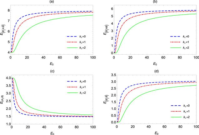
Figure 1. The bipartite entanglement as a function of the strength of a constant electric field E0 for different transverse momentums k⊥. The parameters are fixed as s = q = m = 1. |
In figure 2, we show the bipartite entanglement as a function of the mass m for different charges q. From figures 2(a)–(b), we can see that the bipartite entanglements ${E}_{(B| A\bar{B})}$ and ${E}_{(\bar{B}| {AB})}$ first reduce and then approach the asymptotic values with increasing mass m, which demonstrates that the smaller mass m is beneficial to the growth of bipartite entanglement. The asymptotic values are found to be
$\begin{eqnarray*}\mathop{\mathrm{lim}}\limits_{m\to \infty }{E}_{(B| A\bar{B})}=4{s}^{2},\mathop{\mathrm{lim}}\limits_{m\to \infty }{E}_{(\bar{B}| {AB})}=0.\end{eqnarray*}$
On the other hand, we consider the effect of the charge q on the bipartite entanglements ${E}_{(B| A\bar{B})}$ and ${E}_{(\bar{B}| {AB})}$. It is shown that the 1 → 2 bipartite entanglement increases with the increase of the charge q; this exhibits that the larger charge q benefits the increase of 1 → 2 bipartite entanglement. For the larger mass m, the bipartite entanglements ${E}_{(B| A\bar{B})}$ and ${E}_{(\bar{B}| {AB})}$ are hard to increase by the charge q. According to the extracted information from the 1 → 2 bipartite entanglement, we find that the smaller mass m and the larger charge q are more conducive to the generation of particle–antiparticle pairs.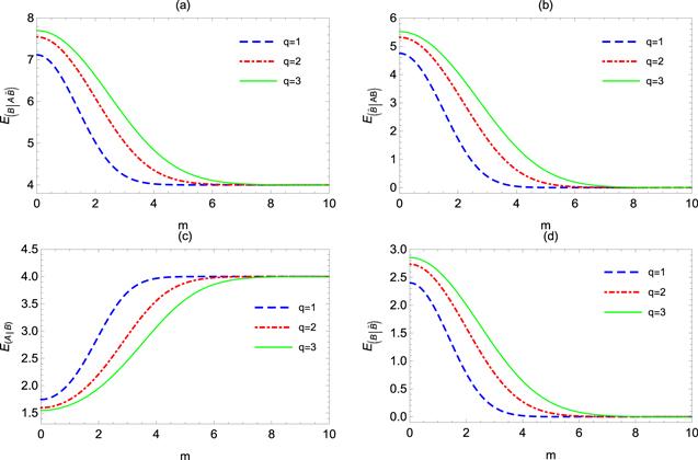
Figure 2. The bipartite entanglement as a function of the mass m for different charges q. The parameters are fixed as s = k⊥ = 1 and E0 = 10. |
In order to better understand the interaction between the initial squeezing and the Schwinger effect via the generation of Gaussian entanglement, we discuss the behavior of 1 → 1 bipartite entanglement in the three-mode system. First of all, taking the trace over mode $\bar{B}$, we obtain the covariance matrix between the modes A and B19 ), we can see that the bipartite entanglement ${E}_{(B| \bar{B})}$ is independent of the initial squeezing.
$\begin{eqnarray}{\sigma }_{{AB}}{\left({\boldsymbol{p}},{\boldsymbol{k}}\right)}^{\mathrm{out}}=\left(\begin{array}{cc}\cosh (2s){I}_{2} & \sinh (2s)\sqrt{1+{{\rm{e}}}^{\tfrac{-\pi ({m}^{2}+{k}_{\perp }^{2})}{{{qE}}_{0}}}}{Z}_{2}\\ \sinh (2s)\sqrt{1+{{\rm{e}}}^{\tfrac{-\pi ({m}^{2}+{k}_{\perp }^{2})}{{{qE}}_{0}}}}{Z}_{2} & \left[{{\rm{e}}}^{\tfrac{-\pi ({m}^{2}+{k}_{\perp }^{2})}{{{qE}}_{0}}}(1+\cosh (2s))+\cosh (2s)\right]{\text{}}{I}_{2}\end{array}\right).\end{eqnarray}$
The contangle quantifying the bipartite entanglement between the modes A and B is found to be $\begin{eqnarray}{E}_{(A| B)}={\mathrm{arcsinh}}^{2}\left[\sqrt{{\left(\displaystyle \frac{1+(1+2{{\rm{e}}}^{\tfrac{\pi ({m}^{2}+{k}_{\perp }^{2})}{{{qE}}_{0}}})\cosh (2s)}{1++2{{\rm{e}}}^{\tfrac{\pi ({m}^{2}+{k}_{\perp }^{2})}{{{qE}}_{0}}}+\cosh (2s)}\right)}^{2}-1}\right].\end{eqnarray}$
In a similar way, we take the trace over mode B and obtain the covariance matrix between the modes A and $\bar{B}$ $\begin{eqnarray}{\sigma }_{A\bar{B}}{\left({\boldsymbol{p}},-{\boldsymbol{k}}\right)}^{\mathrm{out}}=\left(\begin{array}{cc}\cosh (2s){I}_{2} & \sinh (2s)\sqrt{{{\rm{e}}}^{\tfrac{-\pi ({m}^{2}+{k}_{\perp }^{2})}{{{qE}}_{0}}}}{I}_{2}\\ \sinh (2s)\sqrt{{{\rm{e}}}^{\tfrac{-\pi ({m}^{2}+{k}_{\perp }^{2})}{{{qE}}_{0}}}}{I}_{2} & \left[{{\rm{e}}}^{\tfrac{-\pi ({m}^{2}+{k}_{\perp }^{2})}{{{qE}}_{0}}}(1+\cosh (2s))+1\right]{\text{}}{I}_{2}\end{array}\right).\end{eqnarray}$
We find that the Gaussian state ${\sigma }_{A\bar{B}}{\left({\boldsymbol{p}},{\boldsymbol{k}}\right)}^{\mathrm{out}}$ is not entangled. (Note that the Schwinger effect can generate the fermionic entanglement between the modes A and $\bar{B}$ [6]). We are also interested in the bipartite entanglement between the modes B and $\bar{B}$ (or particle and the antiparticle). Tracing over the mode A, we obtain the covariance matrix between the modes B and $\bar{B}$ $\begin{eqnarray}{\sigma }_{B\bar{B}}{\left({\boldsymbol{k}},-{\boldsymbol{k}}\right)}^{\mathrm{out}}=\left(\begin{array}{cc}{\sigma }_{B}{I}_{2} & {{ \mathcal E }}_{B\bar{B}}{Z}_{2}\\ {{ \mathcal E }}_{B\bar{B}}{Z}_{2} & {\sigma }_{\bar{B}}{I}_{2}\end{array}\right),\end{eqnarray}$
where ${\sigma }_{B}=\left[{{\rm{e}}}^{\tfrac{-\pi ({m}^{2}+{k}_{\perp }^{2})}{{{qE}}_{0}}}(1+\cosh (2s))+\cosh (2s)\right]$, ${\sigma }_{\bar{B}}\,=\left[{{\rm{e}}}^{\tfrac{-\pi ({m}^{2}+{k}_{\perp }^{2})}{{{qE}}_{0}}}(1+\cosh (2s))+1\right]$ and ${{ \mathcal E }}_{B\bar{B}}=2\sinh (2s)\sqrt{{{\rm{e}}}^{\tfrac{-\pi ({m}^{2}+{k}_{\perp }^{2})}{{{qE}}_{0}}}}\times \sqrt{{{\rm{e}}}^{\tfrac{-\pi ({m}^{2}+{k}_{\perp }^{2})}{{{qE}}_{0}}}+1}.$ The contangle between the modes B and $\bar{B}$ is found to be $\begin{eqnarray}{E}_{(B| \bar{B})}={\mathrm{arcsinh}}^{2}\left[2\sqrt{{{\rm{e}}}^{\tfrac{-\pi ({m}^{2}+{k}_{\perp }^{2})}{{{qE}}_{0}}}}\sqrt{{{\rm{e}}}^{\tfrac{-\pi ({m}^{2}+{k}_{\perp }^{2})}{{{qE}}_{0}}}+1}\right].\end{eqnarray}$
From equation (From figures 1(c)–(d), we find that, with the increase of the strength E0, the bipartite entanglement E(A∣B) first decreases and then appears an asymptotic value, while the bipartite entanglement ${E}_{(B| \bar{B})}$ increases to an asymptotic value; this means that the strength E0 reduces quantum entanglement between particles, and generates quantum entanglement between particle–antiparticle pairs. When E0 → ∞ , we obtain
$\begin{eqnarray*}\begin{array}{l}\mathop{\mathrm{lim}}\limits_{{E}_{0}\to \infty }{E}_{(A| B)}={\mathrm{arcsinh}}^{2}\left[\sqrt{{\left(\displaystyle \frac{1+3\cosh (2s)}{3+\cosh (2s)}\right)}^{2}-1}\right],\\ \mathop{\mathrm{lim}}\limits_{{E}_{0}\to \infty }{E}_{(B| \bar{B})}={\mathrm{arcsinh}}^{2}\left[2\sqrt{2}\right].\end{array}\end{eqnarray*}$
From figures 1(c)–(d), we also find that, with the growth of the transverse momentum k⊥, the bipartite entanglement E(A∣B) increases, while the bipartite entanglement ${E}_{(B| \bar{B})}$ decreases; this means that the larger momentum k⊥ protects quantum entanglement between particles, but it suppresses quantum entanglement between particle–antiparticle pairs.From figures 2(c)–(d), we can see that, with increasing the mass m, the bipartite entanglement E(A∣B) increases to an asymptotic value 4s2, while the bipartite entanglement ${E}_{(B| \bar{B})}$ decreases to zero; this means that the larger mass m is favorable to the protection of quantum entanglement between particles, but unfavorable to the enhancement of quantum entanglement between particle–antiparticle pairs. On the other hand, with the increase of the charge q, the bipartite entanglement E(A∣B) decreases, while the bipartite entanglement ${E}_{(B| \bar{B})}$ increases; this means that the larger charge q accelerates the decrease of the entanglement between particles, and the increase of the entanglement between particle–antiparticle pairs. Compared with the 1 → 1 entanglement ${E}_{(B| \bar{B})}$ between particle–antiparticle pairs, the 1 → 2 entanglements ${E}_{(B| A\bar{B})}$ and ${E}_{(\bar{B}| {AB})}$ are more sensitive to the strength E0, the momentum k⊥, the mass m and the charge q. Therefore, it is easier to extract information from the 1 → 2 entanglement than from the 1 → 1 entanglement. When s → 0, we obtain
$\begin{eqnarray*}\mathop{\mathrm{lim}}\limits_{s\to 0}{E}_{(B| A\bar{B})}=\mathop{\mathrm{lim}}\limits_{s\to 0}{E}_{(\bar{B}| {AB})}={E}_{(B| \bar{B})}.\end{eqnarray*}$
4.2. Generation of genuine tripartite entanglement
For any three-mode Gaussian state, an appropriate measure of genuine tripartite entanglement is available. The measure is called the residual contangle that is derived from the monogamy inequality in equation (9 ). According to the definition in equation (10 ), the genuine tripartite entanglement is found to be
$\begin{eqnarray}\begin{array}{l}{E}_{(A| B| \bar{B})}=4{s}^{2}\\ \,-{\mathrm{arcsinh}}^{2}\left[\sqrt{{\left(\displaystyle \frac{1+(1+2{{\rm{e}}}^{\tfrac{\pi ({m}^{2}+{k}_{\perp }^{2})}{{{qE}}_{0}}})\cosh (2s)}{1++2{{\rm{e}}}^{\tfrac{\pi ({m}^{2}+{k}_{\perp }^{2})}{{{qE}}_{0}}}+\cosh (2s)}\right)}^{2}-1}\right].\end{array}\end{eqnarray}$
For any nonzero value of parameters, the genuine tripartite entanglement quantified by the residual contangle is nonzero value. This shows that the Gaussian state ${\sigma }_{{AB}\bar{B}}{\left({\boldsymbol{p}},{\boldsymbol{k}},-{\boldsymbol{k}}\right)}^{\mathrm{out}}$ is genuinely entangled and contains genuine tripartite entanglement.We plot the genuine tripartite entanglement ${E}_{(A| B| \bar{B})}$ as a function of the strength E0 for different transverse momentums k⊥ in figure 3(a), and as a function of the mass m for different charges q in figure 3 (b). From figure 3 (a), we find that the genuine tripartite entanglement increases from zero to an asymptotic value with the increases of the strength E0. The smaller the momentum k⊥ is, the more favorable the entanglement is. However, the asymptotic value does not depend on the momentum k⊥ and is found to be
$\begin{eqnarray*}\mathop{\mathrm{lim}}\limits_{{E}_{0}\to \infty }{E}_{(A| B| \bar{B})}=4{s}^{2}-{\mathrm{arcsinh}}^{2}\left[\sqrt{{\left(\displaystyle \frac{1+3\cosh (2s)}{3+\cosh (2s)}\right)}^{2}-1}\right].\end{eqnarray*}$
On the other hand, in figure 3 (b), we find that the genuine tripartite entanglement decreases to zero with the increase of the mass m. The larger charge q slows the fall of genuine tripartite entanglement. Therefore, the larger strength E0 and charge q, and the smaller momentum k⊥ and mass m are more conducive to the increase of genuine tripartite entanglement.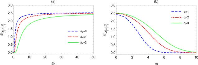
Figure 3. (a) Genuine tripartite entanglement ${E}_{(A| B| \bar{B})}$ as a function of the strength of a constant electric field E0 for different transverse momentums k⊥ and fixed s = q = m = 1. (b) Genuine tripartite entanglement ${E}_{(A| B| \bar{B})}$ as a function of the mass m for different charges q, and fixed s = k⊥ = 1 and E0 = 10. |
In summary, we come to three conclusions: (i) the effect of the strength E0 on quantum entanglement is similar to that of the charge q; (ii) the effect of the transverse momentum k⊥ on quantum entanglement is similar to that of the mass m; (iii) the effect of the strength E0 (charge q) on quantum entanglement is opposite to that of the mass m (transverse momentum k⊥).
5. Quantum entanglement for continuous variables in a pulsed electric field
In the previous section, we studied Gaussian entanglement in a constant electric field. We will continue to study Gaussian entanglement in a pulsed electric field. The gauge potential Aμ becomes
$\begin{eqnarray}{A}_{\mu }=\left[0,0,0,-{E}_{0}\tau \tanh \left(\displaystyle \frac{t}{\tau }\right)\right],\end{eqnarray}$
where $E(t)={E}_{0}{{\rm{sech}} }^{2}\left(\tfrac{t}{\tau }\right)$ is a Sauter-type electric field assumed to be along the z-direction, and τ is the width of the pulsed electric field [5]. Solving the the Klein–Gordon equation in a pulsed electric field, the Bogoliubov coefficients read $\begin{eqnarray}| {\alpha }_{{\boldsymbol{k}}}{| }^{2}=\displaystyle \frac{\cosh [\pi \tau ({\omega }_{{\boldsymbol{k}}}^{\mathrm{in}}+{\omega }_{{\boldsymbol{k}}}^{\mathrm{out}})]+\cosh (2\pi \lambda )}{2\sinh (\pi \tau {\omega }_{{\boldsymbol{k}}}^{\mathrm{in}})\sinh (\pi \tau {\omega }_{{\boldsymbol{k}}}^{\mathrm{out}})},\end{eqnarray}$
$\begin{eqnarray}| {\beta }_{{\boldsymbol{k}}}{| }^{2}=\displaystyle \frac{\cosh [\pi \tau (-{\omega }_{{\boldsymbol{k}}}^{\mathrm{in}}+{\omega }_{{\boldsymbol{k}}}^{\mathrm{out}})]+\cosh (2\pi \lambda )}{2\sinh (\pi \tau {\omega }_{{\boldsymbol{k}}}^{\mathrm{in}})\sinh (\pi \tau {\omega }_{{\boldsymbol{k}}}^{\mathrm{out}})},\end{eqnarray}$
where $\begin{eqnarray*}\begin{array}{rcl}\lambda & = & \sqrt{{\left({{qE}}_{0}{\tau }^{2}\right)}^{2}-\displaystyle \frac{1}{4}},\\ {\omega }_{{\boldsymbol{k}}}^{\mathrm{in}} & = & \sqrt{{\left({k}_{z}+{{qE}}_{0}\tau \right)}^{2}+{k}_{\perp }^{2}+{m}^{2}},\\ {\omega }_{{\boldsymbol{k}}}^{\mathrm{out}} & = & \sqrt{{\left({k}_{z}-{{qE}}_{0}\tau \right)}^{2}+{k}_{\perp }^{2}+{m}^{2}}.\end{array}\end{eqnarray*}$
The calculations in a constant electric field can be applied to a pulsed electric field, but now ∣αk∣2 and ∣βk∣2 are given in equations (22 ) and (23 ), which are inserted into equation (A3 ) in the appendix . Employing equations (8 ) and (10 ), we obtain the forms for the bipartite 1 → 2 entanglement and genuine tripartite entanglement
$\begin{eqnarray}\begin{array}{l}{E}_{(A| B\bar{B})}=4{s}^{2},\\ {E}_{(B| A\bar{B})}\\ ={\mathrm{arcsinh}}^{2}\left[\sqrt{{\left(\cosh (2s)| {\alpha }_{{\boldsymbol{k}}}{| }^{2}+| {\beta }_{{\boldsymbol{k}}}{| }^{2}\right)}^{2}-1}\right],\\ {E}_{(\bar{B}| {AB})}\\ ={\mathrm{arcsinh}}^{2}\left[\sqrt{{\left(| {\alpha }_{{\boldsymbol{k}}}{| }^{2}+\cosh (2s)| {\beta }_{{\boldsymbol{k}}}{| }^{2}\right)}^{2}-1}\right],\\ {E}_{(A| B| \bar{B})}=4{s}^{2}\\ -{\mathrm{arcsinh}}^{2}\left[\sqrt{{\left(\displaystyle \frac{2| {\beta }_{{\boldsymbol{k}}}{| }^{2}+2\cosh (2s)(| {\alpha }_{{\boldsymbol{k}}}{| }^{2}+1)}{2\cosh (2s)| {\beta }_{{\boldsymbol{k}}}{| }^{2}+2(| {\alpha }_{{\boldsymbol{k}}}{| }^{2}+1)}\right)}^{2}-1}\right].\end{array}\end{eqnarray}$
The effect of the pulsed electric field on the bipartite 1 → 2 entanglement and genuine tripartite entanglement is shown in figure 4, which exhibits its dependence on the strength E0 and the width τ. From figures 4(a)–(c), we find that, for E0 smaller than a certain value, the maximum entanglement can be obtained by choosing the optimal width τ of the pulsed electric field. The maximum entanglement depends on the strength E0. From figures 4(d)–(f), we can also find that, for E0 larger than a certain value, the bipartite 1 → 2 entanglement and genuine tripartite entanglement increase to an asymptotic value which depends on the strength E0.
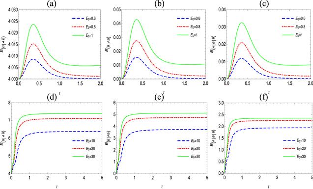
Figure 4. Quantum entanglement as a function of the width τ for different strengths E0. The parameters are fixed as s = q = m = kz = k⊥ = 1. |
In figure 5, we plot the bipartite 1 → 2 entanglement and genuine tripartite entanglement as functions of the momentum kz and the width τ for different E0. From figures 5 (a)–(c), we find that, for E0 = 1, one can choose the optimal momentum kz and width τ to get the maximum bipartite 1 → 2 entanglement and genuine tripartite entanglement. Next, let us consider the case of the strength E0 = 5 in figures 5 (d)–(f). For τ smaller than a certain value, we can obtain the maximum entanglement by choosing the optimal momentum kz. For τ larger than a certain value, we choose the momentum kz close to zero to obtain the larger entanglement.

Figure 5. Quantum entanglement (a)–(c) for E0 = 1 and quantum entanglement (d)–(f) for E0 = 5 as functions of the momentum kz and the width τ. The parameters are fixed as s = q = m = k⊥ = 1. |
Finally, we study how the influence of the pulsed electric field affects the bipartite 1 → 1 entanglement. Through the calculations given in equation (8 ), we get the analytical expressions of bipartite 1 → 1 entanglement
$\begin{eqnarray}\begin{array}{l}{E}_{(A| B)}\\ ={\mathrm{arcsinh}}^{2}\left[\sqrt{{\left(\displaystyle \frac{2| {\beta }_{{\boldsymbol{k}}}{| }^{2}+2\cosh (2s)(| {\alpha }_{{\boldsymbol{k}}}{| }^{2}+1)}{2\cosh (2s)| {\beta }_{{\boldsymbol{k}}}{| }^{2}+2(| {\alpha }_{{\boldsymbol{k}}}{| }^{2}+1)}\right)}^{2}-1}\right],\\ {E}_{(A| \bar{B})}=0,\\ {E}_{(B| \bar{B})}={\mathrm{arcsinh}}^{2}\left[2| {\alpha }_{{\boldsymbol{k}}}| | {\beta }_{{\boldsymbol{k}}}| \right].\end{array}\end{eqnarray}$
Figure 6 shows how the width τ of the pulsed electric field influences the bipartite 1 → 1 entanglement for different strengths E0. In figures 6 (a)–(b), we find that, for E0 smaller than a certain value, one can choose the optimal width τ to get the minimum entanglement E(A∣B) between particles and the maximum entanglement ${E}_{(B| \bar{B})}$ between particle–antiparticle pairs. In figures 6 (c)–(d), we also find that, for E0 larger than a certain value, the width τ reduces entanglement E(A∣B) and increases entanglement ${E}_{(B| \bar{B})}$ to the asymptotic values. In addition, the asymptotic values of entanglement depend on the strength E0.
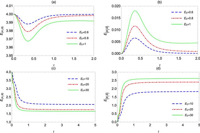
Figure 6. The bipartite 1 → 1 entanglement as a function of the width τ for different strengths E0 and fixed s = q = m = kz = k⊥ = 1. |
In figure 7, we plot the bipartite 1 → 1 entanglement as functions of the momentum kz and the width τ for different E0. From figures 7 (a)–(b), we can see that, for E0 = 1, the minimum entanglement E(A∣B) and the maximum entanglement ${E}_{(B| \bar{B})}$ can be obtained by choosing the optimal momentum kz and width τ. From figures 7 (c)–(d), we can also see that, for E0 = 5, one chooses the optimal momentum kz to obtain the minimum entanglement E(A∣B) and the maximum entanglement ${E}_{(B| \bar{B})}$ for τ smaller than a certain value, and chooses the momentum kz close to zero to get the smaller entanglement E(A∣B) and the larger entanglement ${E}_{(B| \bar{B})}$ for τ larger than a certain value. Combined figures 4–7, the 1 → 2 entanglement between particle and particle–antiparticle pairs are more sensitive to the parameters than the 1 → 1 entanglement between particle–antiparticle pairs.

Figure 7. Quantum entanglement (a)–(b) for E0 = 1 and quantum entanglement (c)–(d) for E0 = 5 as functions of the momentum kz and the width τ. The parameters are fixed as s = q = m = k⊥ = 1. |
It should be noted that the effects of the mass m and the transverse momentum k⊥ on quantum entanglement in a constant electric field are similar to that in a pulsed electric field, and the effect of the charge q on quantum entanglement is similar to that of the strength E0. Therefore, there is no need to elaborate on the influences of the mass m, the transverse momentum k⊥ and the charge q on quantum entanglement in a pulsed electric field. Through the above analysis, we obtain two results: (i) for smaller strength E0 and charge q, we choose the smaller mass m and transverse momentum k⊥, and the optimal momentum kz and width τ to obtain the maximum of the generated entanglement; (ii) for larger strength E0 and charge q, we choose the smaller mass m and transverse momentum k⊥ and momentum kz, and the larger width τ to get the larger value of the generated entanglement. These conditions are more conducive to the generation of particle–antiparticle pairs in a pulsed electric field.
6. Conclusions
In this paper, we have shown that the Schwinger effect generates quantum entanglement for continuous variables. The generated entanglement encodes information about the Schwinger effect. Through the analysis of the generated entanglement, we can extract relevant information that is helpful to guide the generation of particle–antiparticle pairs in future experiments.
We describe the Schwinger effect as a Gaussian channel. Then, we consider a two-mode squeezed state via the Gaussian channel into a three-mode Gaussian state. We study the behaviors of the generated 1 → 1 bipartite entanglement, the generated 1 → 2 bipartite entanglement and genuine tripartite entanglement under the influence of the Schwinger effect. It should be noted that the generated 1 → 2 bipartite entanglement is more sensitive to the Schwinger effect than the generated 1 → 1 bipartite entanglement. Therefore, we choose the generated 1 → 2 bipartite entanglement to extract the optimal parameters more conveniently.
According to the analysis of the generated entanglement, we have found that the smaller transverse momentum k⊥ and mass, the larger strength and charge are easier to generate particle–antiparticle pairs in a constant electric field. For the pulsed electric fields, there are two cases: (i) for smaller strength and charge, the very small mass and transverse momentum k⊥, and the optimal momentum kz and width are beneficial for generating particle–antiparticle pairs; (ii) for larger strength and charge, the smaller mass, the smaller transverse momentum k⊥ and momentum kz, and the larger width are the better conditions for generating particle–antiparticle pairs. These results are favorable to generate particle–antiparticle pairs in experiments.
The fermionic Schwinger effect has not been observed experimentally so far. Although the bosonic Schwinger effect is more difficult to observe experimentally, its theoretical development has been progressing [5, 7, 9]. The Bogoliubov coefficients of the fermion case satisfy the relation ∣αk∣2 + ∣βk∣2 = 1, resulting that ∣αk∣2 decreases towards 0 and ∣βk∣2 is constrained to increase towards 1. The Bogoliubov coefficients of the boson case satisfy another type of relationship ∣αk∣2 − ∣βk∣2 = 1. Therefore, the differences between Bose–Einstein and Fermi–Dirac statistics lead to different behaviors of the Bogoliubov coefficients. In addition, the Bogoliubov coefficients in Rindler spacetime satisfy the relations ${\left(1-{{\rm{e}}}^{-\tfrac{\omega }{T}}\right)}^{-1}-{\left({{\rm{e}}}^{\tfrac{\omega }{T}}-1\right)}^{-1}=1$ for the boson case and ${\left({{\rm{e}}}^{-\tfrac{\omega }{T}}+1\right)}^{-1}+{\left({{\rm{e}}}^{\tfrac{\omega }{T}}+1\right)}^{-1}=1$ for the fermion case, where T is the Unruh temperature [12–17]. Therefore, the different Bogoliubov coefficients between the Schwinger effect and the Unruh effect may lead to different properties of quantum entanglement. For example, quantum entanglement between particle–antiparticle modes may increase non-monotonically with the strength E0 [6], while quantum entanglement between particle–antiparticle modes in Rindler spacetime increases monotonically with the Unruh temperature T [15, 21].
The thermal Schwinger process would be the possible observation of particle–antiparticle pairs production in quantum electrodynamics (QED). It would open up the controlled investigation of particle–antiparticle pairs production. On the experimental side of strong-field QED, the generation of high-intensity lasers provides the possibility to study qualitatively new phenomena in QED [41, 42]. Recently, a mesoscopic simulation of the Schwinger effect has been carried out in graphene devices [43]. Therefore, the optimal parameters extracted from quantum entanglement are beneficial for guiding future simulations and experiments of the Schwinger effect.
Acknowledgments
This work is supported by the National Natural Science Foundation of China (Grant Nos. 12205133, LJKQZ20222315 and 2021BSL013).
Declaration of competing interest
The authors declare that they have no known competing financial interests or personal relationships that could have appeared to influence the work reported in this paper.
Appendix. The final Gaussian state of the entire three-mode system
Equation (6 ) can be expressed as a simpler form
$\begin{eqnarray*}\begin{array}{l}| {0}_{{\boldsymbol{k}}},{0}_{-{\boldsymbol{k}}}{\rangle }^{\mathrm{in}}={U}_{B,\bar{B}}({\boldsymbol{k}},-{\boldsymbol{k}})| {0}_{{\boldsymbol{k}}},{0}_{-{\boldsymbol{k}}}{\rangle }^{\mathrm{out}}\\ \quad ={Q}_{B,\bar{B}}({\boldsymbol{k}},-{\boldsymbol{k}}){P}_{B,\bar{B}}({\boldsymbol{k}},-{\boldsymbol{k}})| {0}_{{\boldsymbol{k}}},{0}_{-{\boldsymbol{k}}}{\rangle }^{\mathrm{out}},\end{array}\end{eqnarray*}$
where ${U}_{B~~,~~\bar{B}}({\boldsymbol{k}}~~,~~-~~{\boldsymbol{k}})~~=~~{Q}_{B~~,~~\bar{B}}({\boldsymbol{k}}~~,~~-~~{\boldsymbol{k} }){P}_{B~~,\bar{B}}( {\boldsymbol{k}}~~,~~-~~{\boldsymbol{k}})$ is a two-mode squeezing operator with ${P}_{B~~,~~\bar{B}}({\boldsymbol{k}}~~,~~-~~{\boldsymbol{k}})\,~~=~~\exp [{\rm{i}}{\text{}}{\theta}_{{\boldsymbol{k}}}({a}_{{\boldsymbol{k}}}^{ \mathrm{out}\dagger}{a}_{{\boldsymbol{k}}}^{\mathrm{out}}\,~~+~~{b}_{{\boldsymbol{k}}}^{\mathrm{out}\dagger}{b}_{{\boldsymbol{k}}}^{\mathrm{out}}+1)]$ and ${Q}_{B~~,~~\bar{B}}({\boldsymbol{k}}~~,~~-~~{\boldsymbol{k}})\,~~=~~\exp[{r}_{{\boldsymbol{k}}}({a}_{{\boldsymbol{k}}}^{\mathrm{out}\dagger }{b}_{{\boldsymbol{k}}}^{\mathrm{out}\dagger }{{\rm{e}}}^{2{\rm{i}}{\vartheta }_{{\boldsymbol{k}}}}\,~~-~~{a}_{{\boldsymbol{k}}}^{\mathrm{out}}{b}_{{\boldsymbol{k}}}^{\mathrm{out}}{{\rm{e}}}^{~~-~~2{\rm{i}}{\vartheta}_{{\boldsymbol{k}}}})]$. By absorbing the squeeze angle and the phase angle,we can rewrite ${U}_{B, \bar{B}}({\boldsymbol{k}} , - {\boldsymbol{k}})$ in the following form $\begin{eqnarray}{U}_{B,\bar{B}}({\boldsymbol{k}},-{\boldsymbol{k}})=\exp [{r}_{{\boldsymbol{k}}}({a}_{{\boldsymbol{k}}}^{\mathrm{out}\dagger }{b}_{{\boldsymbol{k}}}^{\mathrm{out}\dagger }-{a}_{{\boldsymbol{k}}}^{\mathrm{out}}{b}_{{\boldsymbol{k}}}^{\mathrm{out}})],\end{eqnarray}$
where ${\alpha }_{{\boldsymbol{k}}}=\cosh {r}_{{\boldsymbol{k}}}$ and ${\beta }_{{\boldsymbol{k}}}=\sinh {r}_{{\boldsymbol{k}}}$ [44, 45]. Note that the two-mode squeezing operator ${U}_{B,\bar{B}}({\boldsymbol{k}},-{\boldsymbol{k}})$ is a Gaussian operation, which preserves the Gaussianity of the input states. Since we work in phase space, the two-mode squeezing operator ${U}_{B,\bar{B}}({\boldsymbol{k}},-{\boldsymbol{k}})$ can be written in the form of symplectic transformation $\begin{eqnarray}{S}_{B,\bar{B}}({\boldsymbol{k}},-{\boldsymbol{k}})=\left(\begin{array}{cc}| {\alpha }_{{\boldsymbol{k}}}| {I}_{2} & | {\beta }_{{\boldsymbol{k}}}| {Z}_{2}\\ | {\beta }_{{\boldsymbol{k}}}| {Z}_{2} & | {\alpha }_{{\boldsymbol{k}}}| {I}_{2}\end{array}\right),\end{eqnarray}$
where I2 is the unity matrix in 2 × 2 space and Z2 is the third Pauli matrix. It is shown that the Schwinger effect corresponds to a Gaussian channel (a bosonic amplification channel).The expression for equation (13 ) of the main manuscript under the phase space describes the entire Gaussian state after the Schwinger effect which corresponds to a squeezing transformation given in equation (A2 ). The covariance matrix of the entire quantum system readsA3 ) take the forms:
$\begin{eqnarray}\begin{array}{l}{\sigma }_{{AB}\bar{B}}{\left({\boldsymbol{p}},{\boldsymbol{k}},-{\boldsymbol{k}}\right)}^{\mathrm{out}}=\left[{I}_{A}({\boldsymbol{p}})\oplus {S}_{B,\bar{B}}({\boldsymbol{k}},-{\boldsymbol{k}})\right]\\ \times \left[{\sigma }_{{AB}}{\left({\boldsymbol{p}},{\boldsymbol{k}}\right)}^{\mathrm{in}}\oplus {I}_{\bar{B}}(-{\boldsymbol{k}})\right]\left[{I}_{A}({\boldsymbol{p}})\oplus {S}_{B,\bar{B}}({\boldsymbol{k}},-{\boldsymbol{k}})\right]{\,}^{{\mathsf{T}}}\\ =\left(\begin{array}{ccc}{{\boldsymbol{\sigma }}}_{A} & {{ \mathcal E }}_{{AB}} & {{ \mathcal E }}_{A\bar{B}}\\ {{ \mathcal E }}_{{AB}}^{{\mathsf{T}}} & {{\boldsymbol{\sigma }}}_{B} & {{ \mathcal E }}_{B\bar{B}}\\ {{ \mathcal E }}_{A\bar{B}}^{{\mathsf{T}}} & {{ \mathcal E }}_{B\bar{B}}^{{\mathsf{T}}} & {{\boldsymbol{\sigma }}}_{\bar{B}}\end{array}\right),\end{array}\end{eqnarray}$
where $\left[{\sigma }_{{AB}}{\left({\boldsymbol{p}},{\boldsymbol{k}}\right)}^{\mathrm{in}}\oplus {I}_{\bar{B}}(-{\boldsymbol{k}})\right]$ is the initial covariance matrix for the entire Gaussian state. The diagonal elements in equation ( $\begin{eqnarray}{{\boldsymbol{\sigma }}}_{A}=\cosh (2s){I}_{2},\end{eqnarray}$
$\begin{eqnarray}{{\boldsymbol{\sigma }}}_{B}=[\cosh (2s)| {\alpha }_{{\boldsymbol{k}}}{| }^{2}+| {\beta }_{{\boldsymbol{k}}}{| }^{2}]{I}_{2},\end{eqnarray}$
and $\begin{eqnarray}{{\boldsymbol{\sigma }}}_{\bar{B}}=[| {\alpha }_{{\boldsymbol{k}}}{| }^{2}+\cosh (2s)| {\beta }_{{\boldsymbol{k}}}{| }^{2}]{I}_{2}.\end{eqnarray}$
The non-diagonal elements have the following forms $\begin{eqnarray}{{ \mathcal E }}_{{AB}}=[| {\alpha }_{{\boldsymbol{k}}}| \sinh (2s)]{Z}_{2},\end{eqnarray}$
$\begin{eqnarray}{{ \mathcal E }}_{B\bar{B}}=[2{\cosh }^{2}(s)| {\alpha }_{{\boldsymbol{k}}}| | {\beta }_{{\boldsymbol{k}}}| ]{Z}_{2},\end{eqnarray}$
and $\begin{eqnarray}{{ \mathcal E }}_{A\bar{B}}=[\sinh (2s)| {\beta }_{{\boldsymbol{k}}}| ]{I}_{2}.\end{eqnarray}$