


1. Introduction
The first successful measurement of a gravitational-wave (GW) signal [1] from a compact binary coalescence by LIGO has marked the dawn of multi-messenger astronomy and opened a new window to probe the Universe [2–4]. GWs are also a powerful tool for testing gravity theory in the strong-field regime. So far, the merger events from LIGO-Virgo-KAGRA (LVK) collaboration can all be well described by general relativity (GR) [5–7].
The no-hair theorem of black holes (BHs) in GR states that a general relativistic BH is completely described by four physical parameters: mass, spin, electric charge, and magnetic charge. If magnetic charges exist in the Universe, they can provide a new unexplored window into fundamental physics in the Standard Model of particle physics. Although no evidence of magnetic charges has been found in the laboratory until now [8, 9], GWs provide a completely different way to test magnetic charges. Magnetically charged BHs have attracted much attention not only in theoretical study but also in recent astronomical observations [10–14]. For instance, [10] discusses the spectacular properties of magnetically charged BHs, showing that the magnetic field near the horizon of the magnetically charged BH can be strong enough to restore the electroweak symmetry. The astrophysical signatures for magnetically charged BHs also have been studied in [13].
Compared with Schwarzschild BHs, charged BHs emit both gravitational and electromagnetic radiation and have rich phenomena. Recently, there has been an increasing interest in charged BHs; see [10–49] and references therein. In the previous papers [12, 14], we studied the case of binary BHs (BBHs) with electric and magnetic charges in circular and elliptical orbits on a cone. On the one hand, using the Newtonian approximation with radiation reactions, we calculate the total emission rate of energy and angular momentum due to gravitational and electromagnetic radiation. In the case of circular orbits, we show that electric and magnetic charges could significantly suppress the merger times of the dyonic binary system. On the other hand, when considering elliptical orbits, we show that the emission rate of energy and angular momentum due to gravitational and electromagnetic radiation have the same dependence on the conic angle for different cases. Not all BBHs are bounded systems and those from encounters with black holes could have positive energy. Therefore, it is important and meaningful to derive the orbit of BBHs with electric and magnetic charges for the unbounded case (i.e. E > 0) and explore their characteristic features.
In this paper, we extend our previous analyses to the unbounded case and derive the hyperbolic orbit of BBHs with electric and magnetic charges. In the Universe, the two-body dynamical capture is an absolutely common and effective way to form BBH systems. We also derive the merger rate of BBHs with electric and magnetic charges from the two-body dynamical capture. The paper is structured as follows. In section 2 , we derive the hyperbolic orbit of BBHs with electric and magnetic charges. In the low-velocity and weak-field regime, by using a Newtonian method, we calculate the total emission rate of energy due to gravitational and electromagnetic radiation from BBHs with electric and magnetic charges in hyperbolic orbits. In section 3 , we develop a formalism to derive the merger rate of BBHs with electric and magnetic charges from dynamical capture via gravitational and electromagnetic radiation. In section 4 , we apply the formalism to find the effects of the charges on the merger rate for the near-extremal case and discover that the effects cannot be ignored. Finally, section 5 is devoted to the conclusion and discussion. Throughout this paper, we set $G=c=4\pi {\varepsilon }_{0}=\tfrac{{\mu }_{0}}{4\pi }=1$ unless otherwise specified.
2. Gravitational and electromagnetic radiation
In this section, we focus on the case that the distance of the dyonic BH binary is much larger than their event horizons. In such a case, the metric is approximately the Minkowski metric. Therefore, it is a good approximation that the dyonic BH binary is described by two massive point-like objects with electric and magnetic charges in the Minkowski spacetime. This approximation has also been employed in recent works [13, 15, 20] that examine charged binary black holes. Recent numerical-relativity simulations validate this approximation when the separation distance between the black hole binary is significantly larger than their event horizons [30]. Before we calculate the total emission rate of energy due to gravitational and electromagnetic radiation from BBHs with electric and magnetic charges, we need to know the hyperbolic orbit. In the following subsection, we will derive the hyperbolic orbit of BBHs with electric and magnetic charges.
2.1. Hyperbolic orbits of BBHs with electric and magnetic charges without radiation
Here, we consider the hyperbolic encounter of two BHs with mass, electric and magnetic charges (m1, q1, g1) and (m2, q2, g2). According to [12, 14], choosing the center of mass system at the origin and considering the Lorentz force and gravitational force, the equation of motion is
$\begin{eqnarray}\mu {\ddot{R}}^{i}=C\displaystyle \frac{{R}^{i}}{{R}^{3}}-D{\epsilon }_{{jk}}^{i}\displaystyle \frac{{R}^{j}}{{R}^{3}}{v}^{k},\end{eqnarray}$
where R is the distance between two dyonic BHs, C = − m1m2 + q1q2 + g1g2, D = q2g1 − g2q1, ${v}^{i}={\dot{R}}^{i}\,={\rm{d}}{R}^{i}/{\rm{d}}t$, and $\mu =\tfrac{{m}_{1}{m}_{2}}{{m}_{1}+{m}_{2}}$ is the reduced mass. Notice that ${q}_{1}^{2}+{g}_{1}^{2}\leqslant {m}_{1}^{2}$ and ${q}_{2}^{2}+{g}_{2}^{2}\leqslant {m}_{2}^{2}$, so C ≤ 0. Following [12, 14], the generalized angular momentum of the binary system L is the Laplace–Runge–Lenz vector defined by ${\boldsymbol{L}}\equiv \tilde{{\boldsymbol{L}}}-D\hat{{\boldsymbol{r}}}$, where $\tilde{{\boldsymbol{L}}}\equiv \mu {\boldsymbol{R}}\times {\boldsymbol{v}}$ is the orbital angular momentum of the binary system and $\hat{{\boldsymbol{r}}}$ is the unit vector along R. It should be noted that one BH with an electric charge and the other BH with a magnetic charge also gives a non-zero D, and therefore the orbits occur on the cone, as will be explained below.Choosing the z-axis along the generalized angular momentum L, the conserved module of the generalized angular momentum and energy are given by2 ), eliminating the parameter t, we can get4 ) as conic-shaped orbits of the binary, which is confined to the surface of a cone with half-aperture angle θ. The orbits are shown in figure 1 by choosing a = 1, e = 2, and $\sin \theta =1/4$. Now we have the hyperbolic orbit, and we will calculate the total emission rates of energy due to gravitational and electromagnetic radiation in the next subsection.
$\begin{eqnarray}\begin{array}{l}L=\displaystyle \frac{\tilde{L}}{\sin \theta }=\mu {R}^{2}\dot{\phi },\\ E=\displaystyle \frac{1}{2}\mu {\dot{R}}^{2}+\displaystyle \frac{{\tilde{L}}^{2}}{2\mu {R}^{2}}+\displaystyle \frac{C}{R},\end{array}\end{eqnarray}$
where θ is a constant determined by $\cos \theta =\tfrac{| D| }{L}$. Throughout this paper, we only consider θ ∈ (0, π/2] for simplify. For θ ∈ [π/2, π), we can refine ${{\boldsymbol{R}}}^{{\prime} }=-{\boldsymbol{R}}$ to make θ ∈ (0, π/2]. From equation ( $\begin{eqnarray}\displaystyle \frac{\dot{\phi }}{\dot{R}}=\displaystyle \frac{{\rm{d}}\phi }{{\rm{d}}R}={\left(\displaystyle \frac{2\mu E}{{L}^{2}}{R}^{4}-\displaystyle \frac{2\mu C}{{L}^{2}}{R}^{3}-{\sin }^{2}\theta {R}^{2}\right)}^{-\tfrac{1}{2}}.\end{eqnarray}$
Adjusting x = 1/R and using the integral $\int \tfrac{{\rm{d}}x}{\sqrt{\alpha +\beta x+\gamma {x}^{2}}}\,=\tfrac{1}{\sqrt{-\gamma }}\arccos \left(-\tfrac{\beta +2\gamma x}{\sqrt{{\beta }^{2}-4\alpha \gamma }}\right)$, we can get one of the solutions as $R=\tfrac{\tfrac{{\tilde{L}}^{2}}{\mu | C| }}{1+\sqrt{1+\tfrac{2{\tilde{L}}^{2}}{\mu {C}^{2}}E}\cos ((\phi -{\phi }_{0})\sin \theta )}$, which is consistent with [12, 14]. Notice the sum, $\arccos (x)+\arccos (-x)$, is a constant, we can get the other branch of solution, $R=\tfrac{\tfrac{{\tilde{L}}^{2}}{\mu | C| }}{1-\sqrt{1+\tfrac{2{\tilde{L}}^{2}}{\mu {C}^{2}}E}\cos ((\phi -{\phi }_{0})\sin \theta )}$. For the hyperbolic case in which E > 0, we choose φ0 = 0 for simplicity. The two solutions result in an identical energy emission rate, so we only consider the second branch of the solution. Therefore, the orbit is explicitly given by $\begin{eqnarray}{\boldsymbol{R}}=\displaystyle \frac{a\left({e}^{2}-1\right)}{1-e\cos (\phi \sin \theta )}\left(\begin{array}{c}\sin \theta \cos \phi \\ \sin \theta \sin \phi \\ \cos \theta \end{array}\right),\end{eqnarray}$
where a and e can be interpreted as the semimajor axis and eccentricity. They are defined by $\begin{eqnarray}a\equiv \left|\displaystyle \frac{C}{2E}\right|=-\displaystyle \frac{C}{2E},\quad e\equiv {\left(1+\displaystyle \frac{2E{\tilde{L}}^{2}}{\mu {C}^{2}}\right)}^{1/2}.\end{eqnarray}$
Since R > 0, we can derive the range as $\phi \in \left({\phi }_{1},\tfrac{2\pi }{\sin \theta }-{\phi }_{1}\right)$, where ${\phi }_{1}=\tfrac{\arccos \left({e}^{-1}\right)}{\sin \theta }$. Noting that θ is a constant determined by the initial condition, we can interpret equation (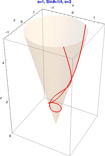
Figure 1. A conic-shaped orbit of the binary that is confined to the surface of a cone by choosing the parameters a = 1, e = 2, and $\sin \theta =1/4$. |
2.2. Gravitational and electromagnetic radiation from BBHs with electric and magnetic charges
In this subsection, we will focus on gravitational and electromagnetic radiation. Let us start by considering gravitational radiation. According to [50], the radiated power of GWs due to gravitational quadrupole radiation, $\tfrac{{\rm{d}}{E}_{\mathrm{GW}}^{\mathrm{quad}}}{{\rm{d}}t}$, is expressed as
$\begin{eqnarray}\begin{array}{rcl}\displaystyle \frac{{\rm{d}}{E}_{\mathrm{GW}}^{\mathrm{quad}}}{{\rm{d}}t} & = & -\displaystyle \frac{1}{5}\left({\dddot{Q}}_{{ij}}{\dddot{Q}}_{{ij}}\right)\\ & = & -\displaystyle \frac{1}{5}\left({\dddot{M}}_{{ij}}{\dddot{M}}_{{ij}}-\displaystyle \frac{1}{3}{\left({\dddot{M}}_{{kk}}\right)}^{2}\right),\end{array}\end{eqnarray}$
where Mij is the second mass moment, and ${Q}_{{ij}}\equiv {M}_{{ij}}-\tfrac{1}{3}{\delta }_{{ij}}{M}_{{kk}}$ is the traceless second mass moment. In our reference frame where L is along the z axis, the second mass moment Mij takes the 3 × 3 matrix form as $\begin{eqnarray}\begin{array}{l}{M}^{{ij}}=\mu {R}_{i}{R}_{j}\\ =\mu {R}^{2}\left(\begin{array}{ccc}{\sin }^{2}\theta {\cos }^{2}\phi & {\sin }^{2}\theta \cos \phi \sin \phi & \sin \theta \cos \theta \cos \phi \\ {\sin }^{2}\theta \cos \phi \sin \phi & {\sin }^{2}\theta {\sin }^{2}\phi & \sin \theta \cos \theta \sin \phi \\ \sin \theta \cos \theta \cos \phi & \sin \theta \cos \theta \sin \phi & {\cos }^{2}\theta \end{array}\right).\end{array}\end{eqnarray}$
From equation (6 ), to obtain the radiated power of GWs, we need to compute the third derivative of Mij. Notice that the components Mij depend on $\phi $, so one way to compute their derivatives is using $\dot{\phi }$ that is given by6 ), we can obtain the radiated power of GWs, $\tfrac{{\rm{d}}{E}_{\mathrm{GW}}^{\mathrm{quad}}}{{\rm{d}}t}$, and the total energy loss due to gravitational quadrupole radiation, ΔEGW,4 ). According to [12] and the appendix , the energy emission rate due to electromagnetic dipole radiation PEM isappendix , the relation between electromagnetic quadrupole radiation and gravitational quadrupole radiation is given by
$\begin{eqnarray}\dot{\phi }=\displaystyle \frac{\tilde{L}}{\mu {R}^{2}\sin \theta }=\displaystyle \frac{\sqrt{-{\rm{C}}}\csc \theta {\left(\mathrm{ecos}(\phi \sin \theta )-1\right)}^{2}}{{a}^{3/2}{\left({e}^{2}-1\right)}^{3/2}\sqrt{\mu }}.\end{eqnarray}$
Then, using the chain rule, ${\dot{M}}_{{ij}}$ in terms of $\dot{\phi }$ is given by ${\dot{M}}_{{ij}}=\tfrac{{\rm{d}}{M}_{{ij}}}{{\rm{d}}\phi }\dot{\phi }$. Moreover, we can extend the same idea to the second and third derivatives. Therefore, we could arrive at $\begin{eqnarray}{\dddot{M}}_{{ij}}=\displaystyle \frac{{\left(-C\right)}^{3/2}{\beta }_{{ij}}}{{a}^{5/2}{\left({e}^{2}-1\right)}^{5/2}\sqrt{\mu }},\end{eqnarray}$
where βij is a function of e, θ, and φ. The components of βij are given by $\begin{eqnarray}\begin{array}{l}{\beta }_{11}=2\csc \theta \cos \phi {\left(\mathrm{ecos}(\phi \sin \theta )-1\right)}^{2}\\ \,\times \left[4\sin \phi (e\cos (\phi \sin \theta )-1)\left(e{\cos }^{2}\theta \cos (\phi \sin \theta )-1\right)\right.\\ \left.+e{\sin }^{3}\theta \cos \phi \sin (\phi \sin \theta )\right],\\ {\beta }_{12}={\beta }_{21}=2\csc \theta {\left(\mathrm{ecos}(\phi \sin \theta )-1\right)}^{2}\\ \,\times \left[2{\sin }^{2}\phi (e\cos (\phi \sin \theta )-1)\left(e{\cos }^{2}\theta \cos (\phi \sin \theta )-1\right)\right.\\ \,-2{\cos }^{2}\phi (e\cos (\phi \sin \theta )-1)\left(e{\cos }^{2}\theta \cos (\phi \sin \theta )-1\right)\\ \left.+e{\sin }^{3}\theta \sin \phi \cos \phi \sin (\phi \sin \theta )\right],\\ {\beta }_{13}={\beta }_{31}=\cot \theta \csc \theta {\left(\mathrm{ecos}(\phi \sin \theta )-1\right)}^{2}\\ \times \left[2e{\sin }^{3}\theta \cos \phi \sin (\phi \sin \theta )+\sin \phi (e\cos (\phi \sin \theta )-1)\right.\\ \left.\,\times (e(2\cos (2\theta )-1)\cos (\phi \sin \theta )-1)\right],\\ {\beta }_{22}=2\csc \theta \sin \phi {\left(\mathrm{ecos}(\phi \sin \theta )-1\right)}^{2}\\ \,\times \left[e{\sin }^{3}\theta \sin \phi \sin (\phi \sin \theta )-4\cos \phi (e\cos (\phi \sin \theta )-1)\right.\\ \left.\,\times \left(e{\cos }^{2}\theta \cos (\phi \sin \theta )-1\right)\right],\\ {\beta }_{23}={\beta }_{32}=\cot \theta \csc \theta {\left(\mathrm{ecos}(\phi \sin \theta )-1\right)}^{2}\\ \times \left[2e{\sin }^{3}\theta \sin \phi \sin (\phi \sin \theta )+\cos \phi (e\cos (\phi \sin \theta )-1)\right.\\ \left.\times ((e-2e\cos (2\theta ))\cos (\phi \sin \theta )+1)\right],\\ {\beta }_{33}=2e{\cos }^{2}\theta \sin (\phi \sin \theta ){\left(e\cos (\phi \sin \theta )-1\right)}^{2}.\end{array}\end{eqnarray}$
Using equation ( $\begin{eqnarray}\displaystyle \frac{{\rm{d}}{E}_{\mathrm{GW}}^{\mathrm{quad}}}{{\rm{d}}t}=\displaystyle \frac{{C}^{3}}{{a}^{5}{\left({e}^{2}-1\right)}^{5}\mu }{{ \mathcal G }}_{1}(\theta ,\phi ,e),\end{eqnarray}$
$\begin{eqnarray}\begin{array}{l}{\rm{\Delta }}{E}_{\mathrm{GW}}^{\mathrm{quad}}={\int }_{-\infty }^{\infty }\displaystyle \frac{{\rm{d}}{E}_{\mathrm{GW}}^{\mathrm{quad}}}{{\rm{d}}t}{\rm{d}}t\\ ={\int }_{{\phi }_{1}}^{2\pi /\sin \theta -{\phi }_{1}}\displaystyle \frac{{\rm{d}}{E}_{\mathrm{GW}}^{\mathrm{quad}}}{{\rm{d}}t}{\left(\displaystyle \frac{{\rm{d}}\phi }{{\rm{d}}t}\right)}^{-1}{\rm{d}}\phi \\ =-\displaystyle \frac{{\left(-C\right)}^{5/2}}{{a}^{7/2}{\left({e}^{2}-1\right)}^{7/2}\sqrt{\mu }}{{ \mathcal G }}_{2}(\theta ,e),\end{array}\end{eqnarray}$
where $\begin{eqnarray}\begin{array}{l}{{ \mathcal G }}_{1}=\displaystyle \frac{{\csc }^{4}\theta }{120}{\left(e\cos (\phi \sin \theta )-1\right)}^{4}\left\{9{e}^{4}\cos (4\phi \sin \theta )\right.\\ +12e\left[e\left(\left(3{e}^{2}+35\right)\cos (2\phi \sin \theta )-7e\cos (3\phi \sin \theta )\right)\right.\\ \left.-21\left({e}^{2}+4\right)\cos (\phi \sin \theta )\right]\\ -2e\cos (4\theta )\left[e(3{e}^{2}\cos (4\phi \sin \theta )\right.\\ +2\left(6{e}^{2}+43\right)\cos (2\phi \sin \theta )\\ +9{e}^{2}-30e\cos (3\phi \sin \theta )+82)\\ \left.-18\left(5{e}^{2}+4\right)\cos (\phi \sin \theta )\right]\\ +\cos (2\theta )\left[3{e}^{4}\cos (4\phi \sin \theta )\right.\\ +4e\left(6\left(28-3{e}^{2}\right)\cos (\phi \sin \theta )\right.\\ +\left.\left(3{e}^{3}-26e\right)\cos (2\phi \sin \theta )-6{e}^{2}\cos (3\phi \sin \theta \right)\\ \left.\left.+9{e}^{4}-136{e}^{2}-360\right]+27{e}^{4}\,+\,444{e}^{2}\,+\,408\right\},\end{array}\end{eqnarray}$
$\begin{eqnarray}\begin{array}{l}{{ \mathcal G }}_{2}=\displaystyle \frac{{\csc }^{4}\theta }{1800}\left\{-15\arccos \left({e}^{-1}\right)\right.\\ \times \left[2\left(15{e}^{4}+323{e}^{2}+308\right){e}^{2}\cos \left(4\theta \right)\right.\\ +\left(-15{e}^{6}+26{e}^{4}+1976{e}^{2}+720\right)\\ \left.\times \cos \left(2\theta \right)-3\left(15{e}^{6}+404{e}^{4}+1104{e}^{2}+272\right)\right]\\ +450\pi {e}^{6}\cos \left(4\theta \right)+4926\sqrt{{e}^{2}-1}{e}^{4}\cos \left(4\theta \right)\\ +9690\pi {e}^{4}\cos \left(4\theta \right)+13658\sqrt{{e}^{2}-1}{e}^{2}\cos \left(4\theta \right)\\ +9240\pi {e}^{2}\cos \left(4\theta \right)+796\sqrt{{e}^{2}-1}\cos \left(4\theta \right)\\ +(-225\pi {e}^{6}-2079\sqrt{{e}^{2}-1}{e}^{4}+390\pi {e}^{4}\\ +20368\sqrt{{e}^{2}-1}{e}^{2}+29640\pi {e}^{2}+22316\sqrt{{e}^{2}-1}\\ +10800\pi )\cos (2\theta )-675\pi {e}^{6}-7005\sqrt{{e}^{2}-1}{e}^{4}\\ -18180\pi {e}^{4}-47130\sqrt{{e}^{2}-1}{e}^{2}\\ \left.-49680\pi {e}^{2}-26640\sqrt{{e}^{2}-1}-12240\pi \right\}.\end{array}\end{eqnarray}$
Now, let us calculate the emission of electromagnetic dipole and quadrupole radiation due to the electric and magnetic charges on the orbit ( $\begin{eqnarray}\displaystyle \frac{{\rm{d}}{E}_{\mathrm{EM}}^{\mathrm{dip}}}{{\rm{d}}t}=-\displaystyle \frac{2{\mu }^{2}({\left({\rm{\Delta }}{\sigma }_{q}\right)}^{2}+{\left({\rm{\Delta }}{\sigma }_{g}\right)}^{2})}{3}{\ddot{R}}^{i}{\ddot{R}}_{i},\end{eqnarray}$
where Δσq = q2/m2 − q1/m1 and Δσg = g2/m2 − g1/m1 are the dipole moments of electric charges and magnetic charges. Hence, the radiated power of electromagnetic waves, $\tfrac{{\rm{d}}{E}_{\mathrm{EM}}^{\mathrm{dip}}}{{\rm{d}}t}$, and the total energy loss due to electromagnetic radiation, ΔEGW, are given by $\begin{eqnarray}\displaystyle \frac{{\rm{d}}{E}_{\mathrm{EM}}^{\mathrm{dip}}}{{\rm{d}}t}=-\displaystyle \frac{({\left({\rm{\Delta }}{\sigma }_{q}\right)}^{2}+{\left({\rm{\Delta }}{\sigma }_{g}\right)}^{2}){C}^{2}}{{a}^{4}{\left({e}^{2}-1\right)}^{4}}{{ \mathcal K }}_{1}(\theta ,\phi ,e)\end{eqnarray}$
$\begin{eqnarray}\begin{array}{l}{\rm{\Delta }}{E}_{\mathrm{EM}}^{\mathrm{dip}}={\int }_{-\infty }^{\infty }\displaystyle \frac{{\rm{d}}{E}_{\mathrm{EM}}^{\mathrm{dip}}}{{\rm{d}}t}{\rm{d}}t\\ ={\int }_{{\phi }_{1}}^{2\pi /\sin \theta -{\phi }_{1}}\displaystyle \frac{{\rm{d}}{E}_{\mathrm{EM}}^{\mathrm{dip}}}{{\rm{d}}t}{\left(\displaystyle \frac{{\rm{d}}\phi }{{\rm{d}}t}\right)}^{-1}{\rm{d}}\phi \\ =-\displaystyle \frac{({\left({\rm{\Delta }}{\sigma }_{q}\right)}^{2}+{\left({\rm{\Delta }}{\sigma }_{g}\right)}^{2}){\left(-C\right)}^{3/2}\sqrt{\mu }}{{a}^{5/2}{\left({e}^{2}-1\right)}^{5/2}}{{ \mathcal K }}_{2}(\theta ,e),\end{array}\end{eqnarray}$
where $\begin{eqnarray}\begin{array}{l}{{ \mathcal K }}_{1}=\displaystyle \frac{{\csc }^{2}\theta }{12}{\left(e\cos (\phi \sin \theta )-1\right)}^{4}\left(2{e}^{2}\cos (2\phi \sin \theta )\right.\\ +{e}^{2}\cos (2\phi \sin \theta +2\theta ))+{e}^{2}\cos (2\theta -2\phi \sin \theta )\\ +2{e}^{2}\cos (2\theta )+2{e}^{2}-8e\cos (\phi \sin \theta )\\ \left.-4e\cos (\phi \sin \theta +2\theta )-4e\cos (2\theta -\phi \sin \theta )+8\right),\end{array}\end{eqnarray}$
$\begin{eqnarray}\begin{array}{l}{{ \mathcal K }}_{2}=\displaystyle \frac{{\csc }^{2}\theta }{36}\left(-3\arccos ({e}^{-1})\left(\left(3{e}^{2}+20\right){e}^{2}\cos (2\theta )\right.\right.\\ \left.+3{e}^{4}\,+\,28{e}^{2}\,+\,16\right)+(9\pi {e}^{4}+55\sqrt{{e}^{2}-1}{e}^{2}\\ +60\pi {e}^{2}+14\sqrt{{e}^{2}-1})\cos (2\theta )+9\pi {e}^{4}\\ \left.\,+55\sqrt{{e}^{2}-1}{e}^{2}\,+\,84\pi {e}^{2}\,+\,86\sqrt{{e}^{2}-1}+48\pi \right).\end{array}\end{eqnarray}$
From the $\begin{eqnarray}\begin{array}{l}\displaystyle \frac{{\rm{d}}{E}_{\mathrm{EM}}^{\mathrm{quad}}}{{\rm{d}}t}\equiv \displaystyle \frac{{\mu }^{2}({\left({q}_{2}/{m}_{2}^{2}+{q}_{1}/{m}_{1}^{2}\right)}^{2}+{\left({g}_{2}/{m}_{2}^{2}+{g}_{1}/{m}_{1}^{2}\right)}^{2})}{4}\\ \times \,\displaystyle \frac{{\rm{d}}{E}_{\mathrm{GW}}^{\mathrm{quad}}}{{\rm{d}}t}.\end{array}\end{eqnarray}$
Furthermore, the contribution of the quadrupole term of electromagnetic radiation is always smaller than the quadrupole term of gravitational radiation. Therefore, the total energy loss due to electromagnetic dipole and quadrupole radiation and gravitational quadrupole radiation is given by $\begin{eqnarray}\begin{array}{l}{\rm{\Delta }}E={\rm{\Delta }}{E}_{\mathrm{EM}}^{\mathrm{dip}}+{\rm{\Delta }}{E}_{\mathrm{EM}}^{\mathrm{quad}}+{\rm{\Delta }}{E}_{\mathrm{GW}}^{\mathrm{quad}}\\ ={\rm{\Delta }}{E}_{\mathrm{EM}}^{\mathrm{dip}}+\left(1+{\rm{\Lambda }}\right){\rm{\Delta }}{E}_{\mathrm{GW}}^{\mathrm{quad}},\end{array}\end{eqnarray}$
where ${\rm{\Lambda }}=\tfrac{{\mu }^{2}({\left({q}_{2}/{m}_{2}^{2}+{q}_{1}/{m}_{1}^{2}\right)}^{2}+{\left({g}_{2}/{m}_{2}^{2}+{g}_{1}/{m}_{1}^{2}\right)}^{2})}{4}$. In this section, we have calculated the total emission rates of energy due to gravitational and electromagnetic radiation from BBHs with electric and magnetic charges in hyperbolic orbits. In the Universe, the two-body dynamical capture is an absolutely common and effective way to form BBH systems. We will derive the merger rate of BBHs with electric and magnetic charges from the two-body dynamical capture in the next section.3. Merger rate of BBHs with electric and magnetic charges from the two-body dynamical capture
If two BHs with electric and magnetic charges are getting closer and closer, the total energy loss due to gravitational and electromagnetic radiation could exceed the orbital kinetic energy. Hence the unbound system cannot escape to infinity anymore and will form a bound binary with negative orbital energy. Therefore, this binary immediately merges through consequent large electromagnetic and gravitational radiation. For such a process, we can estimate the cross section and calculate the merger rate of BBHs with electric and magnetic charges from the two-body dynamical capture.
Let us consider the interaction of two dyonic BHs with masses and charges (m1, q1, g1) and (m2, q2, g2), and assume that they have an initial relative velocity v, the impact parameter b and the distance of periastron rp. According to the definition of rp and the orbit (4 ), we have ${r}_{{\rm{p}}}\equiv {R}_{{\rm{\min }}}=R\left(\phi =\tfrac{\pi }{\sin \theta }\right)=a(e-1)$. We could approximate the trajectory of a close encounter by the hyperbolic with e → 1 since when the two dyonic BHs pass by closer and closer, the true trajectory is physically indistinguishable from a parabolic one near the periastron where electromagnetic and gravitational radiation dominantly occurs. According to section 2 , the total energy loss due to electromagnetic radiation and gravitational radiation by the close encounter can be evaluated by using e → 1 and the periastron rp ≡ a(e − 1), namely25 ) and (26 ), when y0 = 0, x0 and z0 are expressed as28 ) and rp ≡ a(e − 1), we can get ${b}^{2}={r}_{{\rm{p}}}^{2}+2{{ar}}_{{\rm{p}}}$. Note that the total energy can be expressed as $E\equiv -\tfrac{C}{2a}=\tfrac{\mu {v}^{2}}{2}$, so $a=-\tfrac{C}{\mu {v}^{2}}$. Therefore, we find the relation between rp and b as30 ) and (31 ), we could obtain the merging cross-section $\sigma =\pi {b}_{\max }^{2},$ where bmax is the maximum impact parameter for the dyonic BHs to form a bound system and is determined by
$\begin{eqnarray}{\rm{\Delta }}{E}_{\mathrm{EM}}^{\mathrm{dip}}+\left(1+{\rm{\Lambda }}\right){\rm{\Delta }}{E}_{\mathrm{GW}}^{\mathrm{quad}}\end{eqnarray}$
where $\begin{eqnarray}\begin{array}{l}{\rm{\Delta }}{E}_{\mathrm{EM}}^{\mathrm{dip}}\\ \quad =-\displaystyle \frac{\pi ({\left({\rm{\Delta }}{\sigma }_{q}\right)}^{2}+{\left({\rm{\Delta }}{\sigma }_{g}\right)}^{2}){\left(-C\right)}^{3/2}\sqrt{\mu }(23\cos (2\theta )+47){\csc }^{2}(\theta )}{48\sqrt{2}{r}_{{\rm{p}}}^{5/2}},\end{array}\end{eqnarray}$
$\begin{eqnarray}\begin{array}{l}{\rm{\Delta }}{E}_{\mathrm{GW}}^{\mathrm{quad}}\\ \quad =-\displaystyle \frac{\pi {\left(-C\right)}^{5/2}(-2707\cos (2\theta )-1292\cos (4\theta )+5385){\csc }^{4}\theta }{960\sqrt{2}\sqrt{\mu }{r}_{{\rm{p}}}^{7/2}}.\end{array}\end{eqnarray}$
The definition of the impact parameter b is the distance from the origin to the asymptotes of the hyperbolic orbit. One asymptote of the hyperbolic orbit is given by $\begin{eqnarray}\begin{array}{rcl}x & = & \mathop{\mathrm{lim}}\limits_{\phi \to {\phi }_{1}}\left(\displaystyle \frac{a\left({e}^{2}-1\right)}{1-e\cos (\phi \sin \theta )}\sin \theta \cos \phi \right)\\ & & -l\sin \theta \cos {\phi }_{1},\end{array}\end{eqnarray}$
$\begin{eqnarray*}\begin{array}{rcl}y & = & \mathop{\mathrm{lim}}\limits_{\phi \to {\phi }_{1}}\left(\displaystyle \frac{a\left({e}^{2}-1\right)}{1-e\cos (\phi \sin \theta )}\sin \theta \sin \phi \right)\\ & & -l\sin \theta \sin {\phi }_{1},\end{array}\end{eqnarray*}$
$\begin{eqnarray*}z=\mathop{\mathrm{lim}}\limits_{\phi \to {\phi }_{1}}\left(\displaystyle \frac{a\left({e}^{2}-1\right)}{1-e\cos (\phi \sin \theta )}\cos \theta \right)-l\cos \theta .\end{eqnarray*}$
Here, when choosing y0 = 0, we can get the solution of l0, $\begin{eqnarray}l=\mathop{\mathrm{lim}}\limits_{\phi \to {\phi }_{1}}\left(\displaystyle \frac{a\left({e}^{2}-1\right)}{1-e\cos (\phi \sin \theta )}\displaystyle \frac{\sin \phi }{\sin {\phi }_{1}}\right).\end{eqnarray}$
From equations ( $\begin{eqnarray}\begin{array}{l}{x}_{0}=\mathop{\mathrm{lim}}\limits_{\phi \to {\phi }_{1}}\left(\displaystyle \frac{a\left({e}^{2}-1\right)}{1-e\cos (\phi \sin \theta )}\sin \theta \cos \phi \right.\\ \left.-\displaystyle \frac{a\left({e}^{2}-1\right)}{1-e\cos (\phi \sin \theta )}\displaystyle \frac{\sin \phi }{\sin {\phi }_{1}}\sin \theta \cos {\phi }_{1}\right)\\ =-a\sqrt{{e}^{2}-1}\csc \left(\arccos ({{\rm{e}}}^{-1})\csc \theta \right),\\ {z}_{0}=\mathop{\mathrm{lim}}\limits_{\phi \to {\phi }_{1}}\left(\displaystyle \frac{a\left({e}^{2}-1\right)}{1-e\cos (\phi \sin \theta )}\cos \theta \right.\\ \left.-\displaystyle \frac{a\left({e}^{2}-1\right)}{1-e\cos (\phi \sin \theta )}\displaystyle \frac{\sin \phi }{\sin {\phi }_{1}}\cos \theta \right)\\ =-a\sqrt{{e}^{2}-1}\cot \theta \cot \left(\arccos ({e}^{-1})\csc \theta \right).\end{array}\end{eqnarray}$
Therefore, we get the point of intersection of the asymptotes and x–z plane, (x0, 0, z0). We denote the vector $\vec{{v}_{1}}$ as ${\vec{v}}_{1}=({x}_{0},0,{z}_{0})$. Using the unit vector along the asymptotes of the hyperbolic orbit, ${\vec{v}}_{2}=\left(\sin \theta \cos {\phi }_{1},\sin \theta \sin {\phi }_{1},\cos \theta \right)$, the impact parameter b is given by $\begin{eqnarray}b=\sqrt{{\vec{v}}_{1}\cdot {\vec{v}}_{1}-{\left({\vec{v}}_{1}\cdot {\vec{v}}_{2}\right)}^{2}}=a\sqrt{{e}^{2}-1},\end{eqnarray}$
which is independent of θ. It shows that no matter whether the orbit is three-dimensional (θ ≠ π/2) or two-dimensional (θ = π/2), we always have $b=a\sqrt{{e}^{2}-1}$. From equation ( $\begin{eqnarray}{b}^{2}={r}_{{\rm{p}}}^{2}-\displaystyle \frac{2{{Cr}}_{{\rm{p}}}}{\mu {v}^{2}}.\end{eqnarray}$
In the limit of a strong electromagnetic and gravitational radiation focusing, i.e. rp ≪ b, then we get the distance of the closest approach rp as $\begin{eqnarray}{r}_{{\rm{p}}}=-\displaystyle \frac{\mu {v}^{2}{b}^{2}}{2C}.\end{eqnarray}$
The condition for the dyonic BHs to form a bound system is that the total energy loss due to electromagnetic and gravitational radiation is larger than the kinetic energy μv2/2, i.e., $\begin{eqnarray}{\rm{\Delta }}E+\displaystyle \frac{\mu {v}^{2}}{2}\lt 0.\end{eqnarray}$
From equations ( $\begin{eqnarray}\begin{array}{l}\displaystyle \frac{\pi ({\rm{\Lambda }}+1){C}^{6}(5385-2707\cos (2\theta )-1292\cos (4\theta )){\csc }^{4}\theta }{120{b}_{\max }^{7}{\mu }^{4}{v}^{7}}\\ +\displaystyle \frac{\pi ({\left({\rm{\Delta }}{\sigma }_{q}\right)}^{2}+{\left({\rm{\Delta }}{\sigma }_{g}\right)}^{2}){C}^{4}(23\cos (2\theta )+47){\csc }^{2}\theta }{12{b}_{\max }^{5}{\mu }^{2}{v}^{5}}=\displaystyle \frac{\mu {v}^{2}}{2}.\end{array}\end{eqnarray}$
Here, we want to remind the reader that θ is a function of bmax and is given by ${\cos }^{2}\theta =\tfrac{{D}^{2}}{{D}^{2}+{\mu }^{2}{v}^{2}{b}_{\max }^{2}}$. Finally, we could achieve the differential merger rate of dyonic BHs from the two-body dynamical capture,28 ) and n(m1, q1, g1) and n(m2, q2, g2) are the comoving average number density of dyonic BHs with mass, electric and magnetic charges (m1, q1, g1) and (m2, q2, g2). In this section, we develop a formalism to derive the merger rate of BBHs with electric and magnetic charges from the two-body dynamical capture. Next, we will apply the formalism to find the effects of the charges on the merger rate for the near-extremal case.
$\begin{eqnarray}\begin{array}{l}{\rm{d}}R\,=\,n({m}_{1},{q}_{1},{g}_{1})n({m}_{2},{q}_{2},{g}_{2})\\ \times \left\langle \sigma v\right\rangle {\rm{d}}{m}_{1}{\rm{d}}{m}_{2}{\rm{d}}{q}_{1}{\rm{d}}{q}_{2}{\rm{d}}{g}_{1}{\rm{d}}{g}_{2}\end{array}\end{eqnarray}$
where $\left\langle \sigma v\right\rangle $ denotes the average over relative velocity distribution with $\sigma =\pi {b}_{\max }^{2}$ in equation (4. Effects of the charges on the merger rate for the near-extremal case
The origin of those BHs with electric and magnetic charges may be the primordial BH (PBH) which are BHs formed in the radiation-dominated era of the early Universe due to the collapse of large energy density fluctuations [51–53]. A PBH can be magnetized by the accretion of monopoles in the early Universe. For instance, PBHs in a strong magnetic field can produce a pair of magnetic monopoles through pair production [9, 54]. The magnetized PBH can also produce a strong magnetic field, which results in the accretion of electric charges [55]. This is the mechanism for BHs to have electric and magnetic charges in the early Universe. Recently, Ref. [32] shows that PBHs can be near-extremal charged. In this section, we will apply the formalism developed in the last section to find the effects of the charges on the merger rate for the near-extremal case. For simplicity, we consider a special model assuming that all PBHs have the same mass MPBH. In such a model, the number density of dyonic PBHs is given by
$\begin{eqnarray}\begin{array}{l}n(m,q,g)=\displaystyle \frac{1}{4}\displaystyle \frac{{f}_{\mathrm{PBH}}{\rho }_{\mathrm{DM}}}{{M}_{\mathrm{PBH}}}\left(\delta \left(\displaystyle \frac{q}{m}-{\iota }_{e}\right)+\delta \left(\displaystyle \frac{q}{m}+{\iota }_{e}\right)\right)\\ \times \left(\delta \left(\displaystyle \frac{g}{m}-{\iota }_{m}\right)+\delta \left(\displaystyle \frac{g}{m}+{\iota }_{m}\right)\right)\delta (m-{M}_{\mathrm{PBH}}),\end{array}\end{eqnarray}$
where ρDM is the dark matter energy density at present, and fPBH is the fraction of PBHs in the dark matter. This model suggests that the part of the Universe under study is charge neutral, but charges are locally separated by some mechanisms found in [20, 55]. Here, we only consider the near-extremal case. In other words, we take ${\iota }_{m}\equiv \sqrt{1-{\iota }_{e}^{2}}$. For simplicity, we choose ιe ≥ 0. In the calculation, we take the Maxwell–Boltzmann distribution $P(v)\propto {v}^{2}\exp \left(-{v}^{2}/{v}_{0}^{2}\right)$ for the velocity distribution of BHs with the most probable velocity v0 = 100 km s–1. For the charge-neutral Schwarzschild BHs, the merger rate of PBH binaries from the two-body capture is ${R}_{\mathrm{Sch}}\approx 1.5\times {10}^{-8}{f}_{\mathrm{PBH}}^{2}{\mathrm{Gpc}}^{-3}{\mathrm{yr}}^{-1}$ that is independent of MPBH and scales as ${f}_{\mathrm{PBH}}^{2}$.To show the effects of charges ιe on the merger rate of PBH binaries from the two-body dynamical capture for the near-extremal case, we define a function of ιe as32 ) it follows ${b}_{\max }\propto {M}_{\mathrm{PBH}}$ and $\sigma \propto {M}_{\mathrm{PBH}}^{2}$, we find that R(ιe) is independent of MPBH and scales as ${f}_{\mathrm{PBH}}^{2}$. Therefore, η(ιe) is independent of MPBH and fPBH and is only a function of ιe. In figure 2, we plot η(ιe) as the function of ιe. From the definition, we find $\eta ({\iota }_{e})=\eta (\sqrt{1-{\iota }_{e}^{2}})$ and show that η(ιe) decreases as ιe increases and reaches the minimum value of $\eta \left(\tfrac{\sqrt{2}}{2}\right)\approx 6.3$ in ${\iota }_{e}\in \left[0,\tfrac{\sqrt{2}}{2}\right]$. For ${\iota }_{e}\in \left[\tfrac{\sqrt{2}}{2},1\right]$, η(ιe) increases as ιe increases and reaches the maximum value of η(1) ≈ 8.4. As shown in figure 2, the effects of the charges on the merger rate for the near-extremal case cannot be ignored. In figure 2, we also show that the averaged merging cross section is always much larger than that corresponding to the event horizon radius. Therefore, the Newtonian approximation is sufficiently accurate.
$\begin{eqnarray}\eta ({\iota }_{e})\equiv \displaystyle \frac{R({\iota }_{e})}{{R}_{\mathrm{Sch}}},\end{eqnarray}$
where R(ιe) is the total merger rate of near-extremal PBH binaries with electric charge-to-mass ratio ιe and RSch is the total merger rate of PBH binaries in charge-neutral case. In this special model, C equals $-{M}_{\mathrm{PBH}}^{2}\left(1\pm {\iota }_{e}^{2}\pm \left(1-{\iota }_{e}^{2}\right)\right)$, and D equals $0,\pm 2{\iota }_{e}\sqrt{1-{\iota }_{e}^{2}}{M}_{\mathrm{PBH}}^{2}$ in different cases as shown in table 1. The total merger rate of near-extremal PBH binaries, R(ιe), is the sum of the merger rate of different cases. Notice that from equation (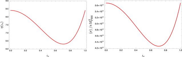
Figure 2. Left: The plot of η(ιe) as a function of ιe. Right: The plot of $\left\langle \sigma \right\rangle /\pi {M}_{\mathrm{PBH}}^{2}$ as a function of ιe. |
Table 1. The value of C and D in different cases. |
| q1 = q2 ≥ 0 | q1 = − q2 ≥ 0 | q1 = q2 < 0 | q1 = − q2 < 0 | |
|---|---|---|---|---|
| g1 = g2 ≥ 0 | C = 0 | $C=-2{\iota }_{e}^{2}{M}_{\mathrm{PBH}}^{2}$ | C = 0 | $C=2{\iota }_{e}^{2}{M}_{\mathrm{PBH}}^{2}$ |
| D = 0 | $D=-2{\iota }_{e}{\iota }_{m}{M}_{\mathrm{PBH}}^{2}$ | D = 0 | $D=-2{\iota }_{e}{\iota }_{m}{M}_{\mathrm{PBH}}^{2}$ | |
| g1 = − g2 ≥ 0 | $C=-2{\iota }_{m}^{2}{M}_{\mathrm{PBH}}^{2}$ | $C=-2{M}_{\mathrm{PBH}}^{2}$ | $C=-2{\iota }_{m}^{2}{M}_{\mathrm{PBH}}^{2}$ | $C=-2{M}_{\mathrm{PBH}}^{2}$ |
| $D=2{\iota }_{e}{\iota }_{m}{M}_{\mathrm{PBH}}^{2}$ | D = 0 | $D=-2{\iota }_{e}{\iota }_{m}{M}_{\mathrm{PBH}}^{2}$ | D = 0 | |
| g1 = g2 < 0 | C = 0 | $C=-2{\iota }_{e}^{2}{M}_{\mathrm{PBH}}^{2}$ | C = 0 | $C=-2{\iota }_{e}^{2}{M}_{\mathrm{PBH}}^{2}$ |
| D = 0 | $D=2{\iota }_{e}{\iota }_{m}{M}_{\mathrm{PBH}}^{2}$ | D = 0 | $D=-2{\iota }_{e}{\iota }_{m}{M}_{\mathrm{PBH}}^{2}$ | |
| g1 = − g2 < 0 | $C=-2{\iota }_{m}^{2}{M}_{\mathrm{PBH}}^{2}$ | $C=-2{M}_{\mathrm{PBH}}^{2}$ | $C=-2{\iota }_{m}^{2}{M}_{\mathrm{PBH}}^{2}$ | $C=-2{M}_{\mathrm{PBH}}^{2}$ |
| $D=-2{\iota }_{e}{\iota }_{m}{M}_{\mathrm{PBH}}^{2}$ | D = 0 | $D=2{\iota }_{e}{\iota }_{m}{M}_{\mathrm{PBH}}^{2}$ | D = 0 |
5. Conclusion
In this work, we have derived the hyperbolic orbit of BBHs with electric and magnetic charges. In the low-velocity and weak-field regime, by using a Newtonian method, we calculate the total emission rate of energy due to gravitational and electromagnetic radiation from BBHs with electric and magnetic charges in hyperbolic orbits. We also develop a formalism to derive the merger rate of BBHs with electric and magnetic charges from the two-body dynamical capture. We apply this formalism to estimate the effects of the charges on the merger rate for the near-extremal case and find that the effects cannot be ignored.
In our calculation, we do not assume the mass of binary. For the solar mass range, combined with [12, 14], the results of this work could provide rich information and a crosscheck to test whether LIGO-Virgo-KAGRA black holes have electric and magnetic charges. On the other hand, those BBHs whose mass is smaller than one solar mass must be PBHs instead of astrophysical BHs. Those extremal charged PBHs are stable and could account for all dark matter without requiring physics beyond the standard model, even though there are many constraints for uncharged PBHs as dark matter [56–58]. Two extremal-charged PBHs with opposite charges could form a bound system through the two-body capture. When they merge, the burst of gamma rays due to the annihilation of charges could be detected by observations.
We find that the BHs with electric and magnetic charges can form a bound system due to gravitational and electromagnetic radiation. Another possibility is that charged BHs do not end up with a bound system in a single encounter but inspiral and enter another scattering event through a hyperbolic encounter. For two BHs with electric and magnetic charges, if the relative velocity or distance is large enough, then the two-body capture cannot happen. These events, however, can generate bursts of GWs. Compared with the GW burst produced by the encounter of Schwarzschild BHs, the GW burst produced by the encounter of BHs with electric and magnetic charges has different characteristics and phenomena. The characteristic peak frequency and detection of such GW bursts is an interesting issue, and we will leave this topic for future work.
Acknowledgments
SPK is supported by the National Research Foundation of Korea (NRF) funded by the Ministry of Education (2019R1I1A3A01063183). LL is supported by the National Natural Science Foundation of China (Grant No. 12247112 and No. 12247176). Z-CC is supported by the National Natural Science Foundation of China (Grant No. 12247176 and No. 12247112) and the China Postdoctoral Science Foundation Fellowship No. 2022M710429.
Electromagnetic dipole and quadrupole radiation from dyonic BBHs
When the differences Δσq of electric charge-to-mass ratios and Δσg of magnetic charge-to-mass ratios are very small or even vanish, the charge quadrupole might be extremely important. Here, we will consider the electromagnetic dipole and quadrupole radiation from dyonic BBHs. We first derive the emission of electromagnetic radiation from electric charges, then calculate the emission from magnetic charges, and finally superimpose their fields.
Following [44], the energy emission due to electromagnetic dipole and quadrupole radiation is given by
$\begin{eqnarray}\displaystyle \frac{{\rm{d}}{E}_{\mathrm{EM}}}{{\rm{d}}t}{| }_{e}=\displaystyle \frac{{\rm{d}}{E}_{\mathrm{EM}}^{\mathrm{dip}}}{{\rm{d}}t}{| }_{e}+\displaystyle \frac{{\rm{d}}{E}_{\mathrm{EM}}^{\mathrm{quad}}}{{\rm{d}}t}{| }_{e},\end{eqnarray}$
and $\begin{eqnarray}\displaystyle \frac{{\rm{d}}{E}_{\mathrm{EM}}^{\mathrm{dip}}}{{\rm{d}}t}{| }_{e}=-\displaystyle \frac{2{\ddot{p}}^{2}}{3},\end{eqnarray}$
$\begin{eqnarray}\displaystyle \frac{{\rm{d}}{E}_{\mathrm{EM}}^{\mathrm{quad}}}{{\rm{d}}t}{| }_{e}=-\displaystyle \frac{{\ddddot{D}}_{{ij}}{\dddot{D}}_{{ij}}}{20}.\end{eqnarray}$
where pi = μΔσqRi is the electric charge dipole and ${D}^{{ij}}=\mu \left(\tfrac{{q}_{1}}{{m}_{1}^{2}}+\tfrac{{q}_{2}}{{m}_{2}^{2}}\right){Q}^{{ij}}$ is the traceless electric charge quadrupole.An important consequence of the enhanced symmetry due to the existence of magnetic monopoles is that the classical dynamics of the charges, fields and Maxwell’s equations are all invariant under the dual transformation,
$\begin{eqnarray}\begin{array}{l}{{\boldsymbol{E}}}^{{\prime} }={\boldsymbol{E}}\cos \alpha -{\boldsymbol{B}}\sin \alpha ,\\ {{\boldsymbol{B}}}^{{\prime} }={\boldsymbol{E}}\sin \alpha +{\boldsymbol{B}}\cos \alpha ,\\ {q}^{{\prime} }=q\cos \alpha +g\sin \alpha ,\\ {g}^{{\prime} }=g\cos \alpha -g\sin \alpha .\end{array}\end{eqnarray}$
Choosing α = π/2, pure electric charges could transform to pure magnetic charges. This helps us to directly find the fields emanating from magnetic charges from the results for pure electric charges. For α = π/2, it is easy to find E2 ∝ B1 and B2 ∝ E1 by labeling the fields from the electric charge, E1, B1, and those from the dual transformation, E2, B2. Now, we consider the integrated energy density on a shell for electric and magnetic fields. Notice that the electric dipole and quadruple have the same direction as the magnetic dipole and quadruple. Therefore, we get E1 ⊥ E2, B1 ⊥ B2, E1∣∣B2, and E2∣∣B1. We then consider the result for the energy density and momentum density $\begin{eqnarray}\begin{array}{l}u=\displaystyle \frac{1}{2}\left({E}^{2}+{B}^{2}\right)\\ =\displaystyle \frac{1}{2}({E}_{1}^{2}+{B}_{1}^{2}+{E}_{2}^{2}+{B}_{2}^{2}\\ +2\left({{\boldsymbol{E}}}_{1}\cdot {{\boldsymbol{E}}}_{2}+{{\boldsymbol{B}}}_{1}\cdot {{\boldsymbol{B}}}_{2}\right))={u}_{1}+{u}_{2},\end{array}\end{eqnarray}$
$\begin{eqnarray}\begin{array}{l}{\boldsymbol{P}}={\boldsymbol{E}}\times {\boldsymbol{B}}={{\boldsymbol{E}}}_{1}\times {{\boldsymbol{B}}}_{1}+{{\boldsymbol{E}}}_{2}\times {{\boldsymbol{B}}}_{2}\\ +{{\boldsymbol{E}}}_{1}\times {{\boldsymbol{B}}}_{2}+{{\boldsymbol{E}}}_{2}\times {{\boldsymbol{B}}}_{1}={{\boldsymbol{P}}}_{1}+{{\boldsymbol{P}}}_{2}.\end{array}\end{eqnarray}$
Using $\tfrac{{\rm{d}}{E}_{\mathrm{EM}}}{{\rm{d}}t}=-{r}^{2}\int {\rm{d}}{\rm{\Omega }}\hat{r}\cdot {\boldsymbol{P}}$, we get $\tfrac{{\rm{d}}{E}_{\mathrm{EM}}}{{\rm{d}}t}=\tfrac{{\rm{d}}{E}_{\mathrm{EM}}}{{\rm{d}}t}{| }_{e}+\tfrac{{\rm{d}}{E}_{\mathrm{EM}}}{{\rm{d}}t}{| }_{m}$. This means that the total energy emissions due to electromagnetic dipole and quadrupole radiation are given by $\begin{eqnarray}\displaystyle \frac{{\rm{d}}{E}_{\mathrm{EM}}}{{\rm{d}}t}=\displaystyle \frac{{\rm{d}}{E}_{\mathrm{EM}}^{\mathrm{dip}}}{{\rm{d}}t}+\displaystyle \frac{{\rm{d}}{E}_{\mathrm{EM}}^{\mathrm{quad}}}{{\rm{d}}t},\end{eqnarray}$
where $\begin{eqnarray}\begin{array}{l}\displaystyle \frac{{\rm{d}}{E}_{\mathrm{EM}}^{\mathrm{dip}}}{{\rm{d}}t}=\displaystyle \frac{{\rm{d}}{E}_{\mathrm{EM}}^{\mathrm{dip}}}{{\rm{d}}t}{| }_{e}+\displaystyle \frac{{\rm{d}}{E}_{\mathrm{EM}}^{\mathrm{dip}}}{{\rm{d}}t}{| }_{m}\\ =-\displaystyle \frac{2{\mu }^{2}({\left({q}_{2}/{m}_{2}-{q}_{1}/{m}_{1}\right)}^{2}+{\left({g}_{2}/{m}_{2}-{g}_{1}/{m}_{1}\right)}^{2})}{3}\\ \times \,{\ddot{R}}^{i}{\ddot{R}}_{i},\end{array}\end{eqnarray}$
$\begin{eqnarray}\begin{array}{l}\displaystyle \frac{{\rm{d}}{E}_{\mathrm{EM}}^{\mathrm{quad}}}{{\rm{d}}t}=\displaystyle \frac{{\rm{d}}{E}_{\mathrm{EM}}^{\mathrm{quad}}}{{\rm{d}}t}{| }_{e}+\displaystyle \frac{{\rm{d}}{E}_{\mathrm{EM}}^{\mathrm{quad}}}{{\rm{d}}t}{| }_{m}\\ =-\displaystyle \frac{{\mu }^{2}({\left({q}_{2}/{m}_{2}^{2}+{q}_{1}/{m}_{1}^{2}\right)}^{2}+{\left({g}_{2}/{m}_{2}^{2}+{g}_{1}/{m}_{1}^{2}\right)}^{2})}{20}\\ \times {\dddot{Q}}_{{ij}}{\dddot{Q}}_{{ij}}.\end{array}\end{eqnarray}$
Notice that $\tfrac{{\rm{d}}{E}_{\mathrm{GW}}^{\mathrm{quad}}}{{\rm{d}}t}\equiv -\tfrac{1}{5}\left({\dddot{Q}}_{{ij}}{\dddot{Q}}_{{ij}}\right)$, we obtain the relation between electromagnetic quadrupole radiation and gravitational quadrupole radiation, $\begin{eqnarray}\begin{array}{l}\displaystyle \frac{{\rm{d}}{E}_{\mathrm{EM}}^{\mathrm{quad}}}{{\rm{d}}t}\equiv \displaystyle \frac{{\mu }^{2}({\left({q}_{2}/{m}_{2}^{2}+{q}_{1}/{m}_{1}^{2}\right)}^{2}+{\left({g}_{2}/{m}_{2}^{2}+{g}_{1}/{m}_{1}^{2}\right)}^{2})}{4}\\ \times \,\displaystyle \frac{{\rm{d}}{E}_{\mathrm{GW}}^{\mathrm{quad}}}{{\rm{d}}t}.\end{array}\end{eqnarray}$
From the metric constraints, ${q}_{1}^{2}+{g}_{1}^{2}\leqslant {m}_{1}^{2}$ and ${q}_{2}^{2}\,+{g}_{2}^{2}\leqslant {m}_{2}^{2}$, it is straightforward to prove that $\tfrac{{\rm{d}}{E}_{\mathrm{EM}}^{i,\mathrm{quad}}}{{\rm{d}}t}\leqslant \tfrac{1}{4}\tfrac{{\rm{d}}{E}_{\mathrm{GW}}^{\mathrm{quad}}}{{\rm{d}}t}$ always holds.