


1. Introduction
In recent years, the quantum effects in plasmas have received more and more attention because of their possible applications [1–5]. Electron spin is one of the important quantum effects in plasma, which may induce significant influence on the interaction of EM wave and plasma. Especially in the case of plasma immersed in a strong external magnetic field, the coupling of electron spin and magnetic field may lead to various important quantum effects [6].
There have been many researches on the spin effects in plasmas. In 2007, Brodin and Marklund [7–9] obtained a set of hydrodynamic equations from the Pauli equation. Based on this set of equations, a series of interesting phenomena have been revealed [10–18]. Nonetheless, these equations are theoretically based on Pauli’s equation, and thus, are nonrelativistic. In addition to these, some studies have also been carried out under the condition of weak relativity [19–21].
In strong laser plasmas, the relativistic effect of electrons is very important in the interaction process. Moreover, in some high-density objects, where the Fermi temperature approaches 0.511 MeV, the electrons near the Fermi surface are also relativistic [22]. In these cases, relativistic effects are significant and cannot be neglected. Therefore, further investigation of electron spin effects in the relativistic case is very important for understanding some physical processes and phenomena in plasmas.
In the condition of strong relativity, Asenjo et al have obtained a set of covariant hydrodynamic equations based on quantum field theory [23]. Nevertheless, this covariant model is very complex to implement in practical situations, notably for numerical applications [19]. In [24], a more succinct hydrodynamic model for strong EM wave–spin plasmas interaction is developed based on the classical Lagrangian function and Euler–Lagrange equation. As a classical model, the quantum statistic effects and quantum diffraction effects are not included in this model. Therefore, this model is applicable for the conditions that the plasma temperature is much higher than the Fermi temperature and the Bohm potential force is much smaller than the spin force. In fact, these conditions are met in astrophysics, Tokamak, high energy laser-plasma systems and many other situations. A comparison of Bohm's potential force and spin force is presented in appendix A .
In the present paper, based on the hydrodynamic model developed in [24], we examine the contribution of spin effects to the EM wave modes in magnetized plasmas in the relativistic case, which has been discussed in the non-relativistic case in [25]. The production of e–p pairs is neglected in the present paper. The dispersion relations of EM wave propagating parallel and perpendicular to the external magnetic field are obtained. Results show that the EM wave modes are obviously affected by the increase of electron effective mass. Additionally, when the EM wave propagates parallel to the external magnetic field, the time component of four-spin amplifies the influence of spin effects on the lower frequency modes. Especially for the left-hand circularly polarized wave, the time component of four-spin leads to a significant change in the dispersion property. Incidentally, the present paper is quite different from [26]. In [26], the propagation properties of extraordinary EM mode in the magnetized quantum plasma are discussed in relativistic situation, however, the influence of relativistic effects on the electron spin is not considered.
2. Basic equations
In order to analyze the spin effects on the strong EM wave in magnetized plasmas, we separate the spin-up and spin-down electrons as two different species of particles. Therefore, the momentum equation and spin equation can be written as [24]
$\begin{eqnarray}\displaystyle \frac{{\rm{d}}({\gamma }_{\alpha }m{{\boldsymbol{U}}}_{\alpha })}{{\rm{d}}t}=-e\left({\boldsymbol{E}}+\displaystyle \frac{1}{c}{{\boldsymbol{U}}}_{\alpha }\times {\boldsymbol{B}}\right)+\displaystyle \frac{e}{{\gamma }_{\alpha }{mc}} \triangledown {{\rm{\Psi }}}_{\alpha },\end{eqnarray}$ 
$\begin{eqnarray}\displaystyle \frac{{\rm{d}}{{\boldsymbol{S}}}_{\alpha }}{{\rm{d}}t}=-\displaystyle \frac{e}{{\gamma }_{\alpha }{mc}}({S}_{\alpha }^{0}{\boldsymbol{E}}+{{\boldsymbol{S}}}_{\alpha }\times {\boldsymbol{B}}),\end{eqnarray}$ 
where, the subscript α = ↑ or ↓ denotes spin-up or spin-down, γα is the relativistic factor, m, e = ∣e∣ and c are the rest mass of the electron, the magnitude of electron charge and the light speed in a vacuum, respectively, Uα is the fluid velocity, E and B are the electric and magnetic fields, Sα and ${S}_{\alpha }^{0}$ are the spatial and time components of the four-spin, and ${{\rm{\Psi }}}_{\alpha }={\gamma }_{\alpha }{{\boldsymbol{S}}}_{\alpha }\cdot \left({\boldsymbol{B}}-\tfrac{1}{c}{{\boldsymbol{U}}}_{\alpha }\times {\boldsymbol{E}}\right)-\tfrac{2{\gamma }_{\alpha }^{2}}{{\gamma }_{\alpha }+1}{S}_{\alpha }^{0}\left(\tfrac{1}{c}{{\boldsymbol{U}}}_{\alpha }\cdot {\boldsymbol{B}}\right)$. The thermal motion and spin flip [27] of electrons are neglected. The curls of the electric and magnetic fields can be written as $\begin{eqnarray} \triangledown \times {\boldsymbol{E}}=-\displaystyle \frac{1}{c}\displaystyle \frac{\partial }{\partial t}{\boldsymbol{B}},\end{eqnarray}$ 
$\begin{eqnarray} \triangledown \times {\boldsymbol{B}}=\displaystyle \frac{4\pi }{c}{\boldsymbol{J}}+\displaystyle \frac{1}{c}\displaystyle \frac{\partial }{\partial t}{\boldsymbol{E}},\end{eqnarray}$ 
where, J = Je + Jm, Je and Jm are the conduction current density and the magnetization current density, respectively.For convenience, we separate the external magnetic field and the wave magnetic field by letting B = B0 + B, and choose a Cartesian coordinate system [12, 25] in which $\hat{{\boldsymbol{z}}}\parallel {{\boldsymbol{B}}}_{0}$, and $\hat{{\boldsymbol{y}}}$ is perpendicular to the plane formed by B0 and k, as shown in figure 1, where ${\boldsymbol{k}}={k}_{\perp }\hat{{\boldsymbol{x}}}+{k}_{\parallel }\hat{{\boldsymbol{z}}}=k\sin \theta \hat{{\boldsymbol{x}}}+k\cos \theta \hat{{\boldsymbol{z}}}$ is the wave vector. For harmonic plane wave solutions, the differential operators ▽ and ∂/∂t are replaced by ik and −i&ohgr;, respectively, where &ohgr; is the frequency of the EM wave. Therefore, equations (3 ) and (4 ) reduce to5 ) into (6 ), we have
$\begin{eqnarray}{\boldsymbol{B}}=\displaystyle \frac{{kc}}{\omega }{\sigma }_{B}{\boldsymbol{E}},\end{eqnarray}$ 
$\begin{eqnarray}{\rm{i}}k{\sigma }_{B}{\boldsymbol{B}}=\displaystyle \frac{4\pi }{c}({{\boldsymbol{J}}}_{e}+{{\boldsymbol{J}}}_{m})-\displaystyle \frac{{\rm{i}}\omega }{c}{\boldsymbol{E}},\end{eqnarray}$ 
where ${\sigma }_{B}=\left(\begin{array}{ccc}0 & -\cos \theta & 0\\ \cos \theta & 0 & -\sin \theta \\ 0 & \sin \theta & 0\end{array}\right)$. Substituting equations ( $\begin{eqnarray}(1+{\eta }^{2}{\sigma }_{B}{\sigma }_{B}){\boldsymbol{E}}=-{\rm{i}}\displaystyle \frac{4\pi }{\omega }({{\boldsymbol{J}}}_{e}+{{\boldsymbol{J}}}_{m}),\end{eqnarray}$ 
where $\eta^2=k^2c^2/\omega^2$.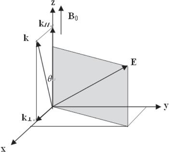
In the Cartesian coordinate system, the conduction current density in equation (7 ) can be written as Je = −e(n↑U↑ + n↓U↓), and can be calculated approximately from the linearization of equation (1 ), i.e.1 ) is neglected considering the fact that ∣Sα∣ ∝ ℏ, ℏ is the Planck’s constant divided by 2π. Therefore9 ) shows that the velocity of fluid is not affected by spin. So, the subscripts α in Uα and γα0 will be omitted in the following. Then, the conduction current density can be written as
$\begin{eqnarray}-{\rm{i}}\omega {\gamma }_{\alpha 0}m{{\boldsymbol{U}}}_{\alpha }=-e\left({\boldsymbol{E}}+\displaystyle \frac{1}{c}{{\boldsymbol{U}}}_{\alpha }\times {{\boldsymbol{B}}}_{0}\right),\end{eqnarray}$
where γα0 is the slow component of relativistic factor, and the last term in equation ( $\begin{eqnarray}{{\boldsymbol{U}}}_{\alpha }=-\displaystyle \frac{{\rm{i}}e}{{\gamma }_{\alpha 0}m\omega (1-{Y}^{2})}{\sigma }_{v}{\boldsymbol{E}},\end{eqnarray}$
where ${\sigma }_{v}=\left(\begin{array}{ccc}1 & -{\rm{i}}Y & 0\\ {\rm{i}}Y & 1 & 0\\ 0 & 0 & 1-{Y}^{2}\end{array}\right)$${\sigma }_{v}=\left(\begin{array}{ccc}1 & -{\rm{i}}Y & 0\\ {\rm{i}}Y & 1 & 0\\ 0 & 0 & 1-{Y}^{2}\end{array}\right)$, $Y=\tfrac{{\rm{\Omega }}}{\omega }=\tfrac{{{eB}}_{0}}{{\gamma }_{~\alpha ~0}~m~\omega~c}$. Equation ( $\begin{eqnarray}{{\boldsymbol{J}}}_{e}=\displaystyle \frac{{\rm{i}}{e}^{2}({n}_{\uparrow }+{n}_{\downarrow })}{{\gamma }_{0}m\omega (1-{Y}^{2})}{\sigma }_{v}{\boldsymbol{E}}.\end{eqnarray}$
The magnetization current density in equation (7 ) can be written as Jm = c∇ × (M↑ + M↓) [7, 9, 16, 25], where M is the magnetization density, and can be calculated approximately from the lowest order of equation (2 ). Letting Sα = Sα0 + Sα, where ${{\boldsymbol{S}}}_{\uparrow 0}=-{{\boldsymbol{S}}}_{\downarrow 0}=({\hslash }/2)\hat{{\boldsymbol{z}}}$, and Sα is the perturbation of spin, the lowest order of the approximation of equation (2 ) givesB . Therefore, using $\langle {S}_{\alpha }^{0}\rangle {\boldsymbol{E}}$ = (1/c)⟨U · Sα⟩E = (1/c)(U* · Sα)E = (1/c)(EU*)Sα and substituting equation (5 ) into equation (11 ), we have13 ) hints that S↑ = −S↓. Therefore, the magnetization current density can be written as [7, 9, 16, 25]B , T and TF are the Bohr magneton, the Boltzmann’s constant, the plasma temperature and the electron Fermi temperature, respectively [17, 25, 28]. Substituting equations (13 ) into (14 ), we have
$\begin{eqnarray}-{\rm{i}}\omega {{\boldsymbol{S}}}_{\alpha }=-\displaystyle \frac{e}{{\gamma }_{0}{mc}}(\langle {S}_{\alpha }^{0}\rangle {\boldsymbol{E}}+{{\boldsymbol{S}}}_{\alpha }\times {{\boldsymbol{B}}}_{0}+{{\boldsymbol{S}}}_{\alpha 0}\times {\boldsymbol{B}}),\end{eqnarray}$ 
where ⟨· · · ⟩ denotes averaging on the high frequencies. Considering the covariant constraint UμSμ = 0, the time component can be obtained as S0 = (1/c)U · S. This result is consistent with the equations of the model developed in [24], as shown in appendix $\begin{eqnarray}\left[1+\displaystyle \frac{{\rm{i}}e}{{\gamma }_{0}m\omega {c}^{2}}({\boldsymbol{E}}{{\boldsymbol{U}}}^{* })+{\rm{i}}Y\sigma \right]{{\boldsymbol{S}}}_{\alpha }=\displaystyle \frac{{\rm{i}}{{eS}}_{\alpha 0}\eta }{{\gamma }_{0}m\omega c}\sigma {\sigma }_{B}{\boldsymbol{E}},\end{eqnarray}$
therefore $\begin{eqnarray}{{\boldsymbol{S}}}_{\alpha }=\displaystyle \frac{{\rm{i}}{{eS}}_{\alpha 0}\eta }{{\gamma }_{0}m\omega c}{\sigma }_{S}\sigma {\sigma }_{B}{\boldsymbol{E}},\end{eqnarray}$
where ${\sigma }_{S}={\left[1+\tfrac{{\rm{i}}e}{{\gamma }_{0}m\omega {c}^{2}}({\boldsymbol{E}}{{\boldsymbol{U}}}^{* })+{\rm{i}}Y\sigma \right]}^{-1}$, $\sigma =\left(\begin{array}{ccc}0 & 1 & 0\\ -1 & 0 & 0\\ 0 & 0 & 0\end{array}\right)$, and U* denotes the complex conjugate of U. Considering S↑0 = −S↓0, equation ( $\begin{eqnarray}{{\boldsymbol{J}}}_{m}=-\displaystyle \frac{e}{m}{\rm{\nabla }}\times ({n}_{\uparrow }{{\boldsymbol{S}}}_{\uparrow }+{n}_{\downarrow }{{\boldsymbol{S}}}_{\downarrow })=-\displaystyle \frac{e}{m}({n}_{\uparrow }-{n}_{\downarrow }) \triangledown \times {{\boldsymbol{S}}}_{\uparrow },\end{eqnarray}$
where (n↑ − n↓) is the difference between spin-up and spin-down electrons locally. In the present paper, a harmonic plane EM wave is considered, and the space variation of electron density is neglected. In the nondegenerate plasmas T ≫ TF, $({n}_{\uparrow }-{n}_{\downarrow })=\tanh \left(\tfrac{{\mu }_{{\rm{B}}}{B}_{0}}{{k}_{{\rm{B}}}T}\right)$, where μB, k $\begin{eqnarray}{{\boldsymbol{J}}}_{m}=\displaystyle \frac{{{ke}}^{2}{\hslash }\eta ({n}_{\uparrow }-{n}_{\downarrow })}{2{\gamma }_{0}{m}^{2}\omega c}{\sigma }_{B}{\sigma }_{S}\sigma {\sigma }_{B}{\boldsymbol{E}}.\end{eqnarray}$
Using equations (10 ) and (15 ) (7 ) reduces to16 ) is consistent with the result in [25]. The dispersion relations of EM wave propagating in arbitrary direction can be obtained from the condition that the determinant of the matrix in equation (16 ) is equal to zero. Incidentally, it is easy to know that the dispersion matrix for the electric field in equation (16 ) is not Hermitian, which hints that the waves are dissipative. Physically, this can be explained by the energy exchange between the EM wave and the spin of the electron.
$\begin{eqnarray}\left[1+{\eta }^{2}{\sigma }_{B}{\sigma }_{B}-\displaystyle \frac{{\omega }_{p}^{2}}{{\gamma }_{0}{\omega }^{2}(1-{Y}^{2})}{\sigma }_{v}+{\rm{i}}\displaystyle \frac{{\omega }_{s}{\eta }^{2}}{{\gamma }_{0}\omega }{\sigma }_{B}{\sigma }_{S}\sigma {\sigma }_{B}\right]{\boldsymbol{E}}=0,\end{eqnarray}$
where ${\omega }_{p}^{2}=\tfrac{4\pi {e}^{2}n}{m}$, ${\omega }_{s}=\tfrac{{\hslash }{\omega }_{p}^{2}({n}_{\uparrow }-{n}_{\downarrow })}{2{{mc}}^{2}n}$, and n = n↑ + n↓. In the non-relativistic case, equation (3. Discussion
3.1. Propagating perpendicular to B0(k⊥B0)
In this situation, θ = π/2 and ${\sigma }_{B}=\left(\begin{array}{ccc}0 & 0 & 0\\ 0 & 0 & -1\\ 0 & 1 & 0\end{array}\right)$, Assuming ${\sigma }_{S}=\left(\begin{array}{ccc}{\sigma }_{S11} & {\sigma }_{S12} & {\sigma }_{S13}\\ {\sigma }_{S21} & {\sigma }_{S22} & {\sigma }_{S23}\\ {\sigma }_{S31} & {\sigma }_{S32} & {\sigma }_{S33}\end{array}\right)$, and substituting σ, σB, σS and σv into equation (16 ), it gives17 ) must vanish. Therefore, two independent relations can be obtained.
$\begin{eqnarray}\left(\begin{array}{ccc}1-\displaystyle \frac{{\omega }_{p}^{2}}{{\gamma }_{0}{\omega }^{2}(1-{Y}^{2})} & \displaystyle \frac{{\rm{i}}Y{\omega }_{p}^{2}}{{\gamma }_{0}{\omega }^{2}(1-{Y}^{2})} & 0\\ -\displaystyle \frac{{\rm{i}}Y{\omega }_{p}^{2}}{{\gamma }_{0}{\omega }^{2}(1-{Y}^{2})} & 1-{\eta }^{2}-\displaystyle \frac{{\omega }_{p}^{2}}{{\gamma }_{0}{\omega }^{2}(1-{Y}^{2})} & {\rm{i}}\displaystyle \frac{{\omega }_{s}{\eta }^{2}}{{\gamma }_{0}\omega }{\sigma }_{S31}\\ 0 & 0 & 1-{\eta }^{2}-\displaystyle \frac{{\omega }_{p}^{2}}{{\gamma }_{0}{\omega }^{2}}-{\rm{i}}\displaystyle \frac{{\omega }_{s}{\eta }^{2}}{{\gamma }_{0}\omega }{\sigma }_{S21}\end{array}\right)\left(\begin{array}{c}{E}_{x}\\ {E}_{y}\\ {E}_{z}\end{array}\right)=0.\end{eqnarray}$
In order to have a nontrivial solution, the determinant of the matrix in equation (The first one is18 ) gives the dispersion relation as,19 ) is the dispersion relation of extraordinary wave mode, and in the non-relativistic case, it is consistent with the result in [25, 26]. In equation (19 ), ${\omega }_{p}^{2}/{\gamma }_{0}=4\pi {e}^{2}n/({\gamma }_{0}m)$ is the frequency of relativistic plasma, and ω = eB0/(γ0mc) is the cyclotron frequency of relativistic electron. If we define the effective mass of the electron m* = γ0m, equation (19 ) shows that the influence of relativistic effect on an extraordinary wave is mainly caused by the increase of electron effective mass.
$\begin{eqnarray}\begin{array}{l}\left[1-{\eta }^{2}-\displaystyle \frac{{\omega }_{p}^{2}}{{\gamma }_{0}{\omega }^{2}(1-{Y}^{2})}\right]\left[1-\displaystyle \frac{{\omega }_{p}^{2}}{{\gamma }_{0}{\omega }^{2}(1-{Y}^{2})}\right]\\ \quad ={\left[\displaystyle \frac{Y{\omega }_{p}^{2}}{{\gamma }_{0}{\omega }^{2}(1-{Y}^{2})}\right]}^{2}.\end{array}\end{eqnarray}$
Equation ( $\begin{eqnarray}{\eta }^{2}=\displaystyle \frac{({\omega }^{2}-{\omega }_{p}^{2}/{\gamma }_{0}-\omega {\rm{\Omega }})({\omega }^{2}-{\omega }_{p}^{2}/{\gamma }_{0}+\omega {\rm{\Omega }})}{{\omega }^{2}({\omega }^{2}-{{\rm{\Omega }}}^{2}-{\omega }_{p}^{2}/{\gamma }_{0})}.\end{eqnarray}$
Equation (The second one is9 ) reduces to23 ) that σS21 = iY/(1 − Y2). Then, substituting σS21 into equation (20 ), the dispersion relation reduces to24 ) is the dispersion relation of the ordinary wave mode, and in the non-relativistic case, it is consistent with the result in [25]. Equation (24 ) shows that the influence of relativistic effect on an ordinary wave is also mainly caused by the increase of electron effective mass.
$\begin{eqnarray}{\eta }^{2}=1-\displaystyle \frac{{\omega }_{p}^{2}}{{\gamma }_{0}{\omega }^{2}}-{\rm{i}}\displaystyle \frac{{\omega }_{s}{\eta }^{2}}{{\gamma }_{0}\omega }{\sigma }_{S21}.\end{eqnarray}$
Generally, the calculation of σS21 is complicated. In the present paper, a simple situation, i.e. Ex = Ey = 0 and Ez ≠ 0, is considered. In this situation, equation ( $\begin{eqnarray}{U}_{z}=-\displaystyle \frac{{\rm{i}}e}{{\gamma }_{0}m\omega }{E}_{z},\end{eqnarray}$
and hence $\begin{eqnarray}\displaystyle \frac{{\rm{i}}e}{{\gamma }_{0}m\omega {c}^{2}}{\boldsymbol{E}}{{\boldsymbol{U}}}^{* }=\left(\begin{array}{ccc}0 & 0 & 0\\ 0 & 0 & 0\\ 0 & 0 & -{U}_{z}{U}_{z}^{* }/{c}^{2}\end{array}\right).\end{eqnarray}$
Therefore $\begin{eqnarray}\begin{array}{l}{\sigma }_{S}={\left(\begin{array}{ccc}1 & {\rm{i}}Y & 0\\ -{\rm{i}}Y & 1 & 0\\ 0 & 0 & 1/{\gamma }_{0}^{2}\end{array}\right)}^{-1}=\displaystyle \frac{1}{1-{Y}^{2}}\\ \quad \times \left(\begin{array}{ccc}1 & -{\rm{i}}Y & 0\\ {\rm{i}}Y & 1 & 0\\ 0 & 0 & {\gamma }_{0}^{2}(1-{Y}^{2})\end{array}\right),\end{array}\end{eqnarray}$
where ${\gamma }_{0}^{2}={\left(1-{U}_{z}{U}_{z}^{* }/{c}^{2}\right)}^{-1}$. It is easy to know from equation ( $\begin{eqnarray}{\eta }^{2}=1-\displaystyle \frac{{\omega }_{p}^{2}}{{\gamma }_{0}{\omega }^{2}}+\displaystyle \frac{Y{\omega }_{s}{\eta }^{2}}{{\gamma }_{0}\omega (1-{Y}^{2})}.\end{eqnarray}$
Equation (3.2. Propagating parallel to B0(k∥B0)
In this case, θ = 0 and ${\sigma }_{B}=\left(\begin{array}{ccc}0 & -1 & 0\\ 1 & 0 & 0\\ 0 & 0 & 0\end{array}\right)$. Substituting σ, σB, σS and σv into equation (16 ), it gives
$\begin{eqnarray}\left(\begin{array}{ccc}1-{\eta }^{2}-\displaystyle \frac{{\omega }_{p}^{2}}{{\gamma }_{0}{\omega }^{2}(1-{Y}^{2})}-{\rm{i}}\displaystyle \frac{{\omega }_{s}{\eta }^{2}}{{\gamma }_{0}\omega }{\sigma }_{S21} & \displaystyle \frac{{\rm{i}}Y{\omega }_{p}^{2}}{{\gamma }_{0}{\omega }^{2}(1-{Y}^{2})}-{\rm{i}}\displaystyle \frac{{\omega }_{s}{\eta }^{2}}{{\gamma }_{0}\omega }{\sigma }_{S22} & 0\\ -\displaystyle \frac{{\rm{i}}Y{\omega }_{p}^{2}}{{\gamma }_{0}{\omega }^{2}(1-{Y}^{2})}+{\rm{i}}\displaystyle \frac{{\omega }_{s}{\eta }^{2}}{{\gamma }_{0}\omega }{\sigma }_{S11} & 1-{\eta }^{2}-\displaystyle \frac{{\omega }_{p}^{2}}{{\gamma }_{0}{\omega }^{2}(1-{Y}^{2})}+{\rm{i}}\displaystyle \frac{{\omega }_{s}{\eta }^{2}}{{\gamma }_{0}\omega }{\sigma }_{S12} & 0\\ 0 & 0 & 1-\displaystyle \frac{{\omega }_{p}^{2}}{{\gamma }_{0}{\omega }^{2}}\end{array}\right)\left(\begin{array}{c}{E}_{x}\\ {E}_{y}\\ {E}_{z}\end{array}\right)=0.\end{eqnarray}$
Similarly, the condition that the determinant of the matrix equals to zero, gives two independent relations.The first one is26 ) shows that the influence of the relativistic effect on the longitudinal electron plasma oscillations is also mainly caused by the increase of electron effective mass.
$\begin{eqnarray}1-\displaystyle \frac{{\omega }_{p}^{2}}{{\gamma }_{0}{\omega }^{2}}=0,\end{eqnarray}$
which corresponds to the longitudinal electron plasma oscillations. In the non-relativistic case, it is consistent with the result in [25]. Equation (The second one is27 ) is difficult. Therefore, we take another method to obtain the dispersion relation in the present paper. Assuming Ez = 0, and using the definition E± = Ex ± iEy (other physical quantities take the same definition), equation (9 ) reduces to
$\begin{eqnarray}\begin{array}{l}\left[1-{\eta }^{2}-\displaystyle \frac{{\omega }_{p}^{2}}{{\gamma }_{0}{\omega }^{2}(1-{Y}^{2})}-{\rm{i}}\displaystyle \frac{{\omega }_{s}{\eta }^{2}}{{\gamma }_{0}\omega }{\sigma }_{S21}\right]\\ \quad \times \left[1-{\eta }^{2}-\displaystyle \frac{{\omega }_{p}^{2}}{{\gamma }_{0}{\omega }^{2}(1-{Y}^{2})}+{\rm{i}}\displaystyle \frac{{\omega }_{s}{\eta }^{2}}{{\gamma }_{0}\omega }{\sigma }_{S12}\right]\\ \quad =\left[\displaystyle \frac{{\rm{i}}Y{\omega }_{p}^{2}}{{\gamma }_{0}{\omega }^{2}(1-{Y}^{2})}-{\rm{i}}\displaystyle \frac{{\omega }_{s}{\eta }^{2}}{{\gamma }_{0}\omega }{\sigma }_{S22}\right]\\ \quad \times \left[-\displaystyle \frac{{\rm{i}}Y{\omega }_{p}^{2}}{{\gamma }_{0}{\omega }^{2}(1-{Y}^{2})}+{\rm{i}}\displaystyle \frac{{\omega }_{s}{\eta }^{2}}{{\gamma }_{0}\omega }{\sigma }_{S11}\right].\end{array}\end{eqnarray}$ 
Generally, the derivation of σS is complicated, and hence, the further calculation of equation ( $\begin{eqnarray}{U}_{\pm }=-\displaystyle \frac{{\rm{i}}e}{{\gamma }_{0}m(\omega \pm {\rm{\Omega }})}{E}_{\pm },\end{eqnarray}$
and the conduction current density can be written as $\begin{eqnarray}{J}_{e\pm }=\displaystyle \frac{{\rm{i}}{e}^{2}({n}_{\uparrow }+{n}_{\downarrow })}{{\gamma }_{0}m(\omega \pm {\rm{\Omega }})}{E}_{\pm },\end{eqnarray}$
where Je = −e(n↑ + n↓)U is used.Considering S0 = (1/c)U · S, we have [24]11 ) [24]31 ), the first γ0 can be regarded to be caused by the increase of electron effective mass, and it suppresses the spin perturbation since γ0 ≥ 1. The second term in the square brackets is caused by ${S}_{\alpha }^{0}$, i.e. the time component of the four-spin. Using ${\gamma }_{0}^{2}\,=1+| a{| }^{2}/{\left(1\pm {\rm{\Omega }}/\omega \right)}^{2}$ and B± = ± iηE±, equation (31 ) reduces to32 ) implies that in a relativistic situation, despite the suppression of the increase of electron effective mass, the spin perturbation is γ0 times larger than the spin perturbation in the non-relativistic situation due to the influence of ${S}_{\alpha }^{0}$. The magnetization current density can be obtained from equation (14 )
$\begin{eqnarray}\langle {S}_{\alpha }^{0}\rangle =\displaystyle \frac{1}{c}\langle {\boldsymbol{U}}\cdot {{\boldsymbol{S}}}_{\alpha }\rangle =\displaystyle \frac{1}{c}({U}_{\pm }^{* }{S}_{\alpha \pm }).\end{eqnarray}$
The spin perturbation can be obtained from equation ( $\begin{eqnarray}{S}_{\alpha \pm }=\mp \displaystyle \frac{{{eS}}_{\alpha 0}}{{\gamma }_{0}{mc}(\omega \pm {\rm{\Omega }})[1-| a{| }^{2}/{\gamma }_{0}^{2}{\left(1\pm {\rm{\Omega }}/\omega \right)}^{2}]}{B}_{\pm },\end{eqnarray}$
where ∣a∣ = ∣eE∣/(m&ohgr;c) is the normalized potential of EM wave. In the denominator of equation ( $\begin{eqnarray}{S}_{\alpha \pm }=-{\rm{i}}\displaystyle \frac{{\gamma }_{0}{{eS}}_{\alpha 0}}{{mc}(\omega \pm {\rm{\Omega }})}\eta {E}_{\pm }.\end{eqnarray}$
Equation ( $\begin{eqnarray}{J}_{m\pm }=\pm \displaystyle \frac{{ke}}{m}({n}_{\uparrow }-{n}_{\downarrow }){S}_{\uparrow \pm }=\mp {\rm{i}}\displaystyle \frac{{\gamma }_{0}{{ke}}^{2}{S}_{\uparrow 0}({n}_{\uparrow }-{n}_{\downarrow })}{{m}^{2}c(\omega \pm {\rm{\Omega }})}\eta {E}_{\pm }.\end{eqnarray}$
Substituting equations (29 ) and (33 ) into (7 ), we have34 )35 ) and (36 ) correspond to the right-hand circularly polarized (RCP) waves and the left-hand circularly polarized (LCP) waves, respectively. In the case of nonrelativistic, equations (35 ) and (36 ) are consistent with the result in [25]. Equations (35 ) and (36 ) show that the dispersion relations of the RCP wave and LCP wave are affected by the time component of four-spin as well as the increase of electron effective mass in the relativistic case. Figure 2 shows the dispersion plots for the RCP and LCP waves mode propagating along the external magnetic field with parameters n = 1036 m−3, B0 = 107 T. Such high-density plasmas immersing in such high magnetic field can be found in the atmosphere of neutron stars and in the interior of white dwarfs [14, 29]. In the numerical calculation, μBB0 ≫ kB T ≫ kB TF are assumed. Therefore, we have $\tanh ({\mu }_{{\rm{B}}}{B}_{0}/{k}_{{\rm{B}}}T)\approx 1$ and ${\omega }_{s}={\hslash }{\omega }_{p}^{2}/(2{{mc}}^{2})$ [25]. In figures 2(a) and (b), the solid curve represents the nonrelativistic case without spin, the short-dash curve represents the nonrelativistic case with spin, the short-dot curve represents the relativistic case but neglects the time component of four-spin, and the dash-dot curve represents the relativistic case and includes the time component of four-spin. Figure 2 hints that the electron spin has no obvious influence on the upper frequency branch, which is consistent with the non-relativistic case [25]. However, the increase of electron effective mass in the relativistic situation affects the upper frequency branch obviously. The main reason is that the increase of electron effective mass leads to the decrease of plasma frequency and electron cyclotron frequency, and thus, the cutoff frequency of the upper frequency branches is decreased. It is evident in the cutoff frequency expressions ${\omega }_{01}=\tfrac{1}{2}({\rm{\Omega }}+\sqrt{{{\rm{\Omega }}}^{2}+4{\omega }_{p}^{2}/{\gamma }_{0}})$ for the RCP wave and ${\omega }_{02}=\tfrac{1}{2}(-{\rm{\Omega }}+\sqrt{{{\rm{\Omega }}}^{2}+4{\omega }_{p}^{2}/{\gamma }_{0}})$ for the LCP wave. Moreover, figure 2 hints that for the lower frequency branch, the increase of electron effective mass suppresses the spin effect, as shown by the short-dot curve in figures 2(a) and (b). However, the time component of four-spin amplifies the spin effect obviously, especially for the LCP wave, as shown by the dash-dot curve in figures 2(a) and (b). The reason is that the spin perturbation can be amplified by the time component of four-spin, as shown in equation (32 ).
$\begin{eqnarray}\left(1-{\eta }^{2}-\displaystyle \frac{{\omega }_{p}^{2}}{{\gamma }_{0}\omega (\omega \pm {\rm{\Omega }})}\pm \displaystyle \frac{{\gamma }_{0}{\omega }_{s}}{(\omega \pm {\rm{\Omega }})}{\eta }^{2}\right){E}_{\pm }=0.\end{eqnarray}$ 
Therefore, two dispersion relations can be obtained from equation ( $\begin{eqnarray}{\eta }^{2}=\left(1-\displaystyle \frac{{\omega }_{p}^{2}}{{\gamma }_{0}\omega (\omega -{\rm{\Omega }})}\right)/\left(1+\displaystyle \frac{{\gamma }_{0}{\omega }_{s}}{\omega -{\rm{\Omega }}}\right),\end{eqnarray}$
$\begin{eqnarray}{\eta }^{2}=\left(1-\displaystyle \frac{{\omega }_{p}^{2}}{{\gamma }_{0}\omega (\omega +{\rm{\Omega }})}\right)/\left(1-\displaystyle \frac{{\gamma }_{0}{\omega }_{s}}{\omega +{\rm{\Omega }}}\right).\end{eqnarray}$
Equations (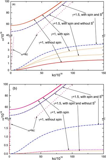
Figure 2. Dispersion plots for the RCP and LCP wave mode. n = 1036 m−3, B0 = 107 T. (a) RCP wave; (b) LCP wave. |
4. Conclusion
In this paper, the spin effects on the dispersion properties of a relativistic strong EM wave propagating in magnetized plasma are discussed based on the hydrodynamic model developed in [24]. As a classical model, the results obtained by this model are reliable in non-degenerate plasmas with negligible Bohm potential force. The dispersion relations of the wave propagating perpendicular and parallel to the external magnetic field are obtained. Results show that the relativistic effects on the dispersion relations of plasma oscillation, ordinary and extraordinary wave modes are mainly induced by the increase of the electron effective mass. When the EM wave propagates parallel to the external magnetic field, the increase of the electron effective mass suppresses the spin effects on the lower frequency branch. However, the time component of the four-spin amplifies the spin effects obviously, especially for the LCP wave.
Appendix A. The comparison of Bohm potential force and spin force
In this part, we give the estimation and comparison of Bohm's potential force and spin force. The Bohm potential force is [30]32 ) and ∣a∣ = ∣eE∣/m&ohgr;c, it is easy to obtain thatA4 ) shows that the ratio increases with the increase of EM wave frequency and decreases with the increase of EM wave intensity. Using the parameters in the present manuscript, i.e. &ohgr; ∼ 1020 s−1, and a ∼ 1, it is easy to estimate that the ratio is approximate to 10−1δn/n0. Therefore, as long as δn ≪ 10n0, the ratio is much smaller than 1 and the Bohm potential can be neglected.
$\begin{eqnarray}{{\boldsymbol{F}}}_{{\rm{B}}}=\tfrac{{\hslash }^{2}}{2\gamma m}{\rm{\nabla }}\left(\tfrac{\bigtriangleup \sqrt{n}}{\sqrt{n}}\right),\end{eqnarray}$
and the lowest approximation of the spin force can be written as $\begin{eqnarray}{{\boldsymbol{F}}}_{S}=\tfrac{e}{{mc}}{\rm{\nabla }}({{\boldsymbol{S}}}_{\alpha }\cdot {\boldsymbol{B}}).\end{eqnarray}$
In Fourier regime, it is easy to obtain that the force induce by Bohm potential is proportional to $\tfrac{{{\hslash }}^{2}{k}^{3}}{4\gamma m}\tfrac{\delta n}{{n}_{0}}$, [31] where n0 and δn represent the background and the perturbation of electron density, respectively. Using equation ( $\begin{eqnarray}{{\boldsymbol{F}}}_{S}\approx \tfrac{1}{2}\gamma {\hslash }\omega k| a{| }^{2},\end{eqnarray}$
where ω ≪ &ohgr; and η ≈ 1 are assumed. So, the ratio of this two term approximately is equal to $\begin{eqnarray}R=| \tfrac{{F}_{{\rm{B}}}}{{F}_{S}}| =\tfrac{\hslash k}{2{mc}}\tfrac{1}{{\gamma }^{2}| a{| }^{2}}\tfrac{\delta n}{{n}_{0}}\approx \tfrac{\hslash \omega }{2{{mc}}^{2}}\tfrac{1}{{\gamma }^{2}| a{| }^{2}}\tfrac{\delta n}{{n}_{0}}.\end{eqnarray}$
Equation (Appendix B. The consistency proof of ${S}^{0}=\tfrac{1}{c}{\boldsymbol{U}}$·S and $\tfrac{{\rm{d}}{S}^{0}}{{\rm{d}}t}=-\tfrac{e}{\gamma {mc}}{\boldsymbol{S}}$·E
In order to verify the consistency, we consider the time derivative of ·S0B3 ) and (B4 ) into (B1 ), we haveB5 ), the second term and the fifth term cancel each other out, and the third term and the fourth term cancel each other out. ThereforeB6 ) is consistent with equation (23) in [24].
$\begin{eqnarray}\tfrac{{\rm{d}}{S}^{0}}{{\rm{d}}t}=\tfrac{1}{c}\tfrac{{\rm{d}}}{{\rm{d}}t}({\boldsymbol{U}}\cdot {\boldsymbol{S}})=\tfrac{1}{c}\left(\tfrac{{\rm{d}}}{{\rm{d}}t}{\boldsymbol{U}}\cdot {\boldsymbol{S}}+{\boldsymbol{U}}\cdot \tfrac{{\rm{d}}}{{\rm{d}}t}{\boldsymbol{S}}\right).\end{eqnarray}$
Considering $\begin{eqnarray}\begin{array}{l}\tfrac{{\rm{d}}}{{\rm{d}}t}(\gamma {\boldsymbol{U}})=\gamma \tfrac{{\rm{d}}}{{\rm{d}}t}{\boldsymbol{U}}+\tfrac{{\rm{d}}\gamma }{{\rm{d}}t}{\boldsymbol{U}}=\gamma \tfrac{{\rm{d}}}{{\rm{d}}t}{\boldsymbol{U}}\\ \quad -\tfrac{e}{{{mc}}^{2}}({\boldsymbol{U}}\cdot {\boldsymbol{E}}){\boldsymbol{U}}=-\tfrac{e}{m}({\boldsymbol{E}}+\tfrac{1}{c}{\boldsymbol{U}}\times {\boldsymbol{B}}),\end{array}\end{eqnarray}$
where equation (16) in [24] is used, and the spin potential and the nonlinear corrections are neglected for simplicity. Therefore $\begin{eqnarray}\tfrac{{\rm{d}}}{{\rm{d}}t}{\boldsymbol{U}}=-\tfrac{e}{\gamma m}({\boldsymbol{E}}+\tfrac{1}{c}{\boldsymbol{U}}\times {\boldsymbol{B}})+\tfrac{e}{\gamma {{mc}}^{2}}({\boldsymbol{U}}\cdot {\boldsymbol{E}}){\boldsymbol{U}}.\end{eqnarray}$
Neglecting the coupling tensor of thermal-spin and the nonlinear corrections, the equation (23) in [24] can be written as $\begin{eqnarray}\tfrac{{\rm{d}}}{{\rm{d}}t}{\boldsymbol{S}}=-\tfrac{e}{\gamma {mc}}({S}^{0}{\boldsymbol{E}}+{\boldsymbol{S}}\times {\boldsymbol{B}}).\end{eqnarray}$
Substituting equations ( $\begin{eqnarray}\begin{array}{l}\tfrac{{\rm{d}}{S}^{0}}{{\rm{d}}t}=-\tfrac{e}{\gamma {mc}}[({\boldsymbol{E}}+\tfrac{1}{c}{\boldsymbol{U}}\times {\boldsymbol{B}}-\tfrac{1}{{c}^{2}}({\boldsymbol{U}}\cdot {\boldsymbol{E}}){\boldsymbol{U}})\cdot {\boldsymbol{S}}\\ \quad +\tfrac{1}{c}{\boldsymbol{U}}\cdot ({S}^{0}{\boldsymbol{E}}+{\boldsymbol{S}}\times {\boldsymbol{B}})].\end{array}\end{eqnarray}$
It is easy to know that in the square brackets of equation ( $\begin{eqnarray}\tfrac{{\rm{d}}{S}^{0}}{{\rm{d}}t}=-\tfrac{e}{\gamma {mc}}{\boldsymbol{S}}\cdot {\boldsymbol{E}}.\end{eqnarray}$
Equation (