


1. Introduction
The two circuit laws established by German scientist Kirchhoff promoted the research and development of circuit theory [1]. Since then, the research of circuit network models has been applied to many subjects. Research shows that they can be employed to model both electrical and non-electrical systems, which has a wide range of applications in physics, material science and graph theory. In many fields of study such as the research of conduction in anisotropic disordered systems [2], random walks and electrical networks [3], resistance distance in network models [4], graphs and networks [5, 6]. Although the research of resistor networks has a history of nearly 180 years, the research progress is slow because of the complex boundary conditions. As is well known, an infinite network does not consider the boundary conditions, so the resistor network is studied from infinite network research. For example, representative studies on infinite resistor networks in literature [7–17] can be seen that these studies have made a lot of progress in large-scale research on resistor network models. In particular, Katsura [18], Cserti [7, 8], Giordano [9], Hijjawi [10], Asad [11–13], and Owaidat [12–17] made important contributions to infinite network research.
The research progress of finite resistor network models is slow because it is limited by boundary conditions. Things took a turn in 2004, when Wu proposed the Laplacian matrix (LM) method [19], and researched a variety of resistor networks with different structures [19]. The key technique of the LM method is to solve the eigenvalues and eigenvectors of the matrix on resistor networks, and then the equivalent resistance is expressed by the eigenvalues and eigenvectors [19–23]. A drawback of the LM method is that it only applies to resistor networks with regular boundaries, which means that the LM method is invalid when the resistance at the boundary is different from the resistance in the network. To achieve a new theoretical breakthrough, Tan (the author himself) finally created a new Recursion-Transform (RT) theory in 2011 after long-term research and thinking, which is used to calculate resistor networks with complex boundary conditions [1]. Shortly after the RT method was established, some new network models were solved, such as three new Cobweb, Globe and Fan network models [24–26]. In 2015, Tan further developed and perfected his RT-I theory (I stands for current) [27–29], where matrix equations used to study resistor networks are established based on current parameters. In 2017, Tan proposed another new RT-V theory to study resistor networks [30], where matrix equations used to study resistor networks are established based on node voltage parameters. Very recently, Tan further summarized the resistance network theory established before and set up the basic principle of m × n resistor networks [31], in which rectangular and cylindrical networks with complex boundaries are solved uniformly. Due to the strong application of RT (RT-V, RT-I) theory, many resistor network models with different structures have been solved by the RT-I theory [32–35], and the electrical properties of various resistance networks are derived from the RT-V theory [36–41]. In order to study complex impedance networks, a variable substitution technique was established in the literature [42], so that a series of RLC complex impedance networks were studied [42–50].
References [25, 37] researched a kind of globe network in terms of the RT-I method, when two poles of the globe network are joined into one pole. [51] refer to it as an apple surface network, and this type of network is shown in figure 1. In the apple network studied in the literature [51], all resistances are regular, such as r1 is at all longitudes and r is at all latitudes. In this paper, we intend to study a special structure of apple surface network with a special boundary, where the boundary resistor connected to the pole O can be a special resistance different from that on the longitude line. The change in boundary conditions will affect the research results. This paper will study the analytical solutions of the potential function of the apple surface network in terms of the RT-V method, and the apple surface network is shown in figure 1.
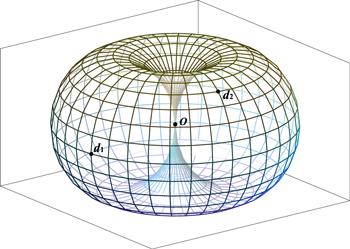
Figure 1. This is an arbitrary m × n apple surface network model, where m and n are the nodal numbers at the longitude (exclude pole O) and latitude, respectively, and the resistance values on the longitude and latitude lines are r0, r1 and r. Detailed parameter descriptions are shown in figure 2. |
The organization of this paper is as follows. In section 2 , we propose the main results of the apple surface network. In section 3 , the main results are derived by the RT-V theory. In section 4 , we discuss the applications of the potential formula and the special cases of the resistance formula. In section 5 , eight visualized images of potential functions are given, and in section 6 a comment is given.
2. The main results
Consider an arbitrary m × n apple surface network with a pair of special boundaries as shown in figure 1 and figure 2, where n and m (excluding node O) are the number of nodes along the latitude and longitude directions, and the resistance on the latitude line is all r, and r1 is the resistance between pole O and adjacent nodes, and the resistance on all longitude lines not adjacent to pole O is r0. In this paper, we only consider the special case of ${r}_{1}={r}_{0}/2,$ which is a new problem that has not been solved before. Assuming the pole $O$ is the origin of the rectangular coordinate system, and a longitude acts as the Y axis as shown in figure 2(a). Denote nodes of the network by coordinate {x, y}, and denote potential of node $d(x,y)$ is ${U}_{m\times n}(x,y)={V}_{x}^{(y)}$ as shown in figure 3. These provisions will apply throughout the text.
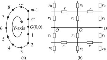
Figure 2. (a) illustrates the distribution of coordinate values by taking a longitude line with m nodes (exclude pole O) as an example. (b) shows that the resistance on the latitude line is all r, and r1 is the resistance between pole O and adjacent nodes, and the resistance on all longitude lines not adjacent to the pole O is r0. And a horizontal wire passing through O can collapse into a pole. |
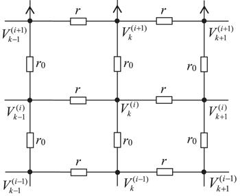
Figure 3. Segment of resistor network with potential parameters. |
In this section, we present two potential function analytical expressions and two equivalent resistance analytical expressions for an arbitrary m × n apple surface network with a special boundary. These results are found for the first time in this paper, which is a theoretical original.
2.1. Analytic expression of potential function
Referring to figures 1 and 2, ${r}_{1}={r}_{0}/2.$ The resistor elements and number of nodes are shown in figure 2. Assuming the current J flows in from ${d}_{1}\left({x}_{1},{y}_{1}\right)$ and flows out from ${d}_{2}\left({x}_{2},{y}_{2}\right),$ and $\left\{{y}_{1},{y}_{2}\right\}\ne 0.$ Selecting ${U}_{m\times n}\left(0,0\right)=0$ as the reference point of potential, the potential of an arbitrary node in the $m\times n$ apple surface network can be written as
$\begin{eqnarray}\begin{array}{l}\displaystyle \frac{{U}_{m\times n}\left(x,y\right)}{J}=\displaystyle \frac{2r}{m}\left(\displaystyle \sum _{i=1}^{m-1}\displaystyle \frac{{g}_{{x}_{1},x}^{\left(i\right)}{S}_{{y}_{1},i}-{g}_{{x}_{2},x}^{\left(i\right)}{S}_{{y}_{2},i}}{{\lambda }_{i}^{n}+{\bar{\lambda }}_{i}^{n}-2}{S}_{y,i}\right.\\ \left.\,+\,\displaystyle \frac{{g}_{{x}_{1},x}^{\left(m\right)}{S}_{{y}_{1},m}-{g}_{{x}_{2},x}^{\left(m\right)}{S}_{{y}_{2},m}}{2\left({\lambda }_{m}^{n}+{\bar{\lambda }}_{m}^{n}-2\right)}{S}_{y,m}\right),\end{array}\end{eqnarray}$ 
where ${S}_{k,i}=\,\sin \left({y}_{k}-\displaystyle \frac{1}{2}\right){\theta }_{i},$ ${\theta }_{i}=i\pi /m,$ and $\begin{eqnarray}{g}_{{x}_{s},x}^{\left(i\right)}={F}_{n-\left|{x}_{s}-x\right|}+{F}_{\left|{x}_{s}-x\right|},{F}_{k}^{(i)}=\left({\lambda }_{i}^{k}-{\bar{\lambda }}_{i}^{k}\right)/\left({\lambda }_{i}-{\bar{\lambda }}_{i}\right),\end{eqnarray}$ 
with $\begin{eqnarray}\begin{array}{l}{\lambda }_{i}=1+v-v\,\cos \,{\theta }_{i}+\sqrt{{\left(1+v-v\,\cos \,{\theta }_{i}\right)}^{2}-1},\\ {\bar{\lambda }}_{i}=1+v-v\,\cos \,{\theta }_{i}-\sqrt{{\left(1+v-v\,\cos \,{\theta }_{i}\right)}^{2}-1},\end{array}\end{eqnarray}$ 
and defining $v=r/{r}_{0},$ where r is the resistor in the latitude lines, and ${r}_{1}={r}_{0}/2$ is the resistance between pole O and adjacent nodes, and the resistance on all longitude lines not adjacent to the pole O is r0.When ${d}_{2}\left({x}_{2},{y}_{2}\right)=O\left(0,0\right),$ and the ${d}_{1}\left({x}_{1},{y}_{1}\right)$ is an arbitrary node, selecting ${U}_{m\times n}\left(0,0\right)=0$ as the reference point of potential, the potential of an arbitrary node in the $m\times n$ apple surface network can be written as
$\begin{eqnarray}\begin{array}{l}\displaystyle \frac{{U}_{m\times n}\left(x,y\right)}{J}\\ \,=\,\displaystyle \frac{2r}{m}\left(\displaystyle \sum _{i=1}^{m-1}\displaystyle \frac{{g}_{{x}_{1},x}^{\left(i\right)}{S}_{{y}_{1},i}}{{\lambda }_{i}^{n}+{\bar{\lambda }}_{i}^{n}-2}{S}_{y,i}+\displaystyle \frac{{g}_{{x}_{1},x}^{\left(m\right)}{S}_{{y}_{1},m}}{2\left({\lambda }_{m}^{n}+{\bar{\lambda }}_{m}^{n}-2\right)}{S}_{y,m}\right).\end{array}\end{eqnarray}$ 
Note that equation (4 ) cannot be reduced from equation (1 ), they are two independent equations. The results show that the expression structure of the potential function is related to whether the external current passes through the pole O.
2.2. Equivalent resistance formula
Refer to figures 1 and 2. The resistor elements and number of nodes are shown in figure 2. Assuming the ${d}_{1}\left({x}_{1},{y}_{1}\right)$ and ${d}_{2}\left({x}_{2},{y}_{2}\right)$ are two arbitrary nodes in figure 1, and $\left\{{y}_{1},{y}_{2}\right\}\ne 0,$ the resistance analytical formula of the $m\times n$ apple surface network can be written as2 ).
$\begin{eqnarray}\begin{array}{l}{R}_{m\times n}\left({d}_{1},{d}_{2}\right)=\displaystyle \frac{2r}{m}\left(\displaystyle \sum _{i=1}^{m-1}\displaystyle \frac{{F}_{n}^{\left(i\right)}\left({S}_{{y}_{1},i}^{2}+{S}_{{y}_{2},i}^{2}\right)-2{g}_{{x}_{2},{x}_{1}}^{\left(i\right)}{S}_{{y}_{1},i}{S}_{{y}_{2},i}}{{\lambda }_{i}^{n}+{\bar{\lambda }}_{i}^{n}-2}\right)\\ \,\,+\,\displaystyle \frac{2r}{m}\left(\displaystyle \frac{{F}_{n}^{\left(m\right)}-{g}_{{x}_{2},{x}_{1}}^{\left(m\right)}\,\cos \left({y}_{1}\pi \right)\cos \left({y}_{2}\pi \right)}{{\lambda }_{m}^{n}+{\bar{\lambda }}_{m}^{n}-2}\right),\end{array}\end{eqnarray}$ 
where ${S}_{k,i}=\,\sin \left({y}_{k}-\tfrac{1}{2}\right){\theta }_{i},$ ${\theta }_{i}=i\pi /m,$ and ${F}_{k}^{(i)}$ and ${g}_{{x}_{2},{x}_{1}}^{(i)}$ are defined in equation (When ${d}_{2}\left({x}_{2},{y}_{2}\right)=O\left(0,0\right),$ the ${d}_{1}\left({x}_{1},{y}_{1}\right)$ is an arbitrary node (${y}_{1}\ne 0$), the resistance analytical formula of the $m\times n$ apple surface network can be written as
$\begin{eqnarray}R\left({d}_{1},O\right)=\displaystyle \frac{2r}{m}\left(\displaystyle \sum _{i=1}^{m-1}\displaystyle \frac{{F}_{n}^{\left(i\right)}{S}_{{y}_{1},i}^{2}}{{\lambda }_{i}^{n}+{\bar{\lambda }}_{i}^{n}-2}+\displaystyle \frac{{F}_{n}^{\left(m\right)}}{2\left({\lambda }_{m}^{n}+{\bar{\lambda }}_{m}^{n}-2\right)}\right).\end{eqnarray}$ 
Note that equation (6 ) cannot be reduced from equation (5 ), they are two independent equations. Why is equation (6 ) special because of the influence of the boundary resistance of ${r}_{1}\ne {r}_{0}.$
3. Method and calculation
In this section, we first derive formulas (1) and (4), and next derive formulas (5) and (6) by the RT-V theory [30]. Next, we will carry out research according to the four basic steps of RT-V theory.
3.1. Modeling the matrix difference equation
Assuming the pole $O$ is the origin of the rectangular coordinate system, and let ${r}_{1}={r}_{0}/2.$ Input current J into the network at ${d}_{1}\left({x}_{1},{y}_{1}\right)$ and exit the current J at ${d}_{2}\left({x}_{2},{y}_{2}\right).$ The node voltage of apple surface network is defined in figure 3, and assuming the potential at the arbitrary node of $d\left(x,y\right)$ is ${U}_{m\times n}\left(x,y\right)={V}_{x}^{\left(y\right)},$ and taking ${V}_{0}^{(0)}=0$ at pole $O.$
First, we focus on nine nodes in figure 3, by Kirchhoff’s law we have $\displaystyle \sum {r}_{i}^{-1}{V}_{k}=0,$ applying it to figure 3, we can obtain the node potential equation as follows by ignoring the external current source:
$\begin{eqnarray*}{V}_{k+1}^{\left(1\right)}=\left(2+3v\right){V}_{k}^{\left(1\right)}-{V}_{k-1}^{\left(1\right)}-v{V}_{k}^{\left(2\right)},i=1\end{eqnarray*}$ 
$\begin{eqnarray*}{V}_{k+1}^{\left(i\right)}=\left(2+2v\right){V}_{k}^{\left(i\right)}-{V}_{k-1}^{\left(i\right)}-v{V}_{k}^{\left(i-1\right)}-v{V}_{k}^{\left(i+1\right)},1\lt i\lt m\end{eqnarray*}$ 
$\begin{eqnarray}{V}_{k+1}^{\left(m\right)}=\left(2+3v\right){V}_{k}^{\left(m\right)}-{V}_{k-1}^{\left(m\right)}-v{V}_{k}^{\left(m-1\right)},i=m\end{eqnarray}$ 
where $v=r/{r}_{0},$ ${r}_{1}={r}_{0}/2.$Next, we consider the input and output conditions of the current J. When $\left({y}_{1},{y}_{2}\right)\ne 0,$ and the current J is injected from ${d}_{1}\left({x}_{1},{y}_{1}\right)$ and exited at ${d}_{2}\left({x}_{2},{y}_{2}\right),$ we obtain (exclude points on the boundary)8 ) cannot contain equation (9 ). However, equations (7) ) and (9 ) can be written in a unified matrix form
$\begin{eqnarray}\begin{array}{l}{V}_{k+1}^{\left(i\right)}=\left(2+2v\right){V}_{k}^{\left(i\right)}-{V}_{k-1}^{\left(i\right)}\\ \,-\,v{V}_{k}^{\left(i-1\right)}-v{V}_{k}^{\left(i+1\right)}-rJ{\delta }_{{x}_{1},k}{\delta }_{{y}_{1},i},\\ {V}_{k+1}^{\left(i\right)}=\left(2+2v\right){V}_{k}^{\left(i\right)}-{V}_{k-1}^{\left(i\right)}\\ \,-\,v{V}_{k}^{\left(i-1\right)}-v{V}_{k}^{\left(i+1\right)}+rJ{\delta }_{{x}_{2},k}{\delta }_{{y}_{2},i}.\end{array}\end{eqnarray}$ 
When $\left\{{y}_{1},{y}_{2}\right\}\ne 0,$ the current J is injected at node of ${d}_{1}\left({x}_{1},1\right)$ and exited at node of ${d}_{2}\left({x}_{2},m\right),$ where ${d}_{1}\left({x}_{1},1\right)$ and ${d}_{2}\left({x}_{2},m\right)$ are points on the boundary, we obtain $\begin{eqnarray}\begin{array}{l}{V}_{k+1}^{\left(1\right)}=\left(2+3v\right){V}_{k}^{\left(1\right)}-{V}_{k-1}^{\left(1\right)}-v{V}_{k}^{\left(2\right)}-rJ{\delta }_{{x}_{1},k}{\delta }_{{y}_{1},i},\\ {V}_{k+1}^{\left(m\right)}=\left(2+3v\right){V}_{k}^{\left(m\right)}-{V}_{k-1}^{\left(m\right)}-v{V}_{k}^{\left(m-1\right)}+rJ{\delta }_{{x}_{2},k}{\delta }_{{y}_{2},i}.\end{array}\end{eqnarray}$ 
Obviously, equation ( $\begin{eqnarray}{\mathop{V}\limits^{ \rightharpoonup }}_{k+1}={A}_{m\times m}{\mathop{V}\limits^{ \rightharpoonup }}_{k}-{\mathop{V}\limits^{ \rightharpoonup }}_{k-1}-r{\mathop{I}\limits^{ \rightharpoonup }}_{x}{\delta }_{y,i},\end{eqnarray}$
where ${\mathop{I}\limits^{ \rightharpoonup }}_{k}$ and ${\mathop{V}\limits^{ \rightharpoonup }}_{k}$ are two $m\times 1$ column matrixes respectively, they are $\begin{eqnarray}{I}_{x}^{\left(i\right)}=J\left({\delta }_{{x}_{1},k}-{\delta }_{{x}_{2},k}\right),\end{eqnarray}$ 
$\begin{eqnarray}{\mathop{V}\limits^{ \rightharpoonup }}_{k}={\left[{V}_{k}^{\left(1\right)}\,,\,{V}_{k}^{\left(2\right)},\,\cdots ,\,{V}_{k}^{\left(m\right)}\right]}^{{\rm{T}}},\end{eqnarray}$ 
and ${\left[\cdot \right]}^{{\rm{T}}}$ denote matrix transpose, the delta function ${\delta }_{x,k}$ means: ${\delta }_{x,k}\left(x=k\right)=1,$ ${\delta }_{x,k}\left(x\ne k\right)=0,$ and matrix ${A}_{m\times m}$ is a tridiagonal matrix, $\begin{eqnarray}{A}_{m\times m}=\left(\begin{array}{ccc}\begin{array}{cc}\left(2+3v\right) & -v\\ -v & \left(2+2v\right)\end{array} & \begin{array}{l}\,0\\ -v\end{array} & \begin{array}{cc}\,0 & \,0\\ \,0 & \,0\end{array}\\ \vdots & \ddots & \vdots \\ \begin{array}{lc}0 & \,0\,\\ 0 & \,0\,\end{array} & \begin{array}{l}-v\\ \,0\end{array} & \begin{array}{cc}\left(2+2v\right) & -v\\ -v & \left(2+3v\right)\end{array}\end{array}\right).\end{eqnarray}$ 
In addition to the above equation, we also need to establish the conditional equations of the left and right boundaries around the Y-axis, one can derive two matrix equations13 ).
$\begin{eqnarray}{\mathop{V}\limits^{ \rightharpoonup }}_{n-1}+{\mathop{V}\limits^{ \rightharpoonup }}_{1}={A}_{m\times m}{\mathop{V}\limits^{ \rightharpoonup }}_{0},\end{eqnarray}$ 
$\begin{eqnarray}{\mathop{V}\limits^{ \rightharpoonup }}_{0}={\mathop{V}\limits^{ \rightharpoonup }}_{n}={A}_{m\times m}{\mathop{V}\limits^{ \rightharpoonup }}_{n-1}-{\mathop{V}\limits^{ \rightharpoonup }}_{n-2},\end{eqnarray}$ 
where matrix ${A}_{m\times m}$ is given by (When ${d}_{2}({x}_{2},{y}_{2})$ is located at pole $O(0,0),$ and the ${d}_{1}({x}_{1},{y}_{1})$ is an arbitrary node, the equations and solutions under this condition will be calculated separately in the following sections.
Above equations (10 )–(15 ) are all equations we need, next we will solve above matrix equations by the RT-V theory.
3.2. Technology of matrix transform
By the third step of the RT-V theory [30], we need to assume a matrix ${P}_{m\times m}$(simply let ${P}_{m\times m}={P}_{m}$), and multiply (10) from the left-hand side using ${P}_{m},$ we have
$\begin{eqnarray}{P}_{m}{\mathop{V}\limits^{ \rightharpoonup }}_{k+1}={P}_{m}{A}_{m}{\mathop{V}\limits^{ \rightharpoonup }}_{k}-{P}_{m}{\mathop{V}\limits^{ \rightharpoonup }}_{k-1}-rJ{P}_{m}{\mathop{I}\limits^{ \rightharpoonup }}_{x}{\delta }_{y,i}.\end{eqnarray}$ 
In order to solve this problem, we need to do a matrix transformation, that is $\begin{eqnarray}{P}_{m}{A}_{m}=\text{diag}\left({t}_{1},{t}_{2},\,\cdots ,\,{t}_{m}\right){P}_{m},\end{eqnarray}$ 
where the diagonal matrix can be derived by $\begin{eqnarray}\det \left|{A}_{m\times m}-t{E}_{m\times m}\right|=0.\end{eqnarray}$ 
By investigation, it is found that matrix ${A}_{m\times m}$ in equation (13 ) is a new matrix which is completely different from the matrices we have seen in the previous article. This is also the focus of innovation in this paper. We figured out its eigenvalues and eigenvectors after a lot of computation and algebra, solving equation (18 ) we get
$\begin{eqnarray}{t}_{i}=2\left(1+v\right)-2v\,\cos \,{\theta }_{i}\,{\rm{with}}\,{\theta }_{i}=i\pi /m.\end{eqnarray}$ 
Substituting (19) into (17), one can derive the eigenvectors of the matrix ${P}_{m\times m}$
$\begin{eqnarray}{P}_{m\times m}=\left(\begin{array}{cc}\begin{array}{cc}\sin \left(\displaystyle \frac{1}{2}{\theta }_{1}\right) & \sin \left(2-\displaystyle \frac{1}{2}\right){\theta }_{1}\\ \sin \left(\displaystyle \frac{1}{2}{\theta }_{2}\right) & \sin \left(2-\displaystyle \frac{1}{2}\right){\theta }_{2}\end{array} & \begin{array}{cc}\cdots & \sin \left(m-\displaystyle \frac{1}{2}\right){\theta }_{1}\\ \cdots & \sin \left(m-\displaystyle \frac{1}{2}\right){\theta }_{2}\end{array}\\ \begin{array}{cc}\vdots & \vdots \\ \sin \left(\displaystyle \frac{1}{2}{\theta }_{m}\right) & \sin \left(2-\displaystyle \frac{1}{2}\right){\theta }_{m}\end{array} & \begin{array}{cc}\ddots & \vdots \\ \cdots & \sin \left(m-\displaystyle \frac{1}{2}\right){\theta }_{m}\end{array}\end{array}\right).\end{eqnarray}$ 
It is found that equation (20 ) is a special matrix whose inverse is not the direct transpose of ${P}_{m\times m},$ that is ${P}_{m\times m}^{-1}\ne \tfrac{2}{m}{\left[{P}_{m\times m}\right]}^{{\rm{T}}}.$ The mth column of the inverse matrix of a matrix ${P}_{m\times m}$ is 1/2 of the row vector value of its mth row. In addition, the rest of the entries of the inverse of ${P}_{m\times m}$ are its transpose. For the sake of expression, let us say ${p}_{k,i}=\,\sin \left(k-\tfrac{1}{2}\right){\theta }_{i},$ ${p}_{k,m}=\,\sin \left(k-\tfrac{1}{2}\right){\theta }_{m},$ then the inverse of ${P}_{m\times m}$ can be written as
$\begin{eqnarray}{P}_{m\times m}^{-1}=\displaystyle \frac{2}{m}\left(\begin{array}{cc}\begin{array}{cc}{p}_{1,1} & {p}_{1,2}\\ {p}_{2,1} & {p}_{2,2}\end{array} & \begin{array}{cc}\cdots & {p}_{1,m-1}\,\displaystyle \frac{1}{2}{p}_{1,m}\\ \cdots & {p}_{2,m-1}\,\displaystyle \frac{1}{2}{p}_{2m}\end{array}\\ \begin{array}{cc}\vdots \, & \vdots \\ {p}_{m,1}\, & {p}_{m,2}\end{array} & \begin{array}{cc}\ddots & \vdots \\ \cdots & {p}_{m,m-1}\,\displaystyle \frac{1}{2}{p}_{m,m}\end{array}\end{array}\right).\end{eqnarray}$ 
The purpose of above calculations is to establish the following transformation relationship,
$\begin{eqnarray}{P}_{m\times m}{\mathop{V}\limits^{ \rightharpoonup }}_{k}={\mathop{X}\limits^{ \rightharpoonup }}_{k}\,{\rm{or}}\,{\mathop{V}\limits^{ \rightharpoonup }}_{k}={\left({P}_{m\times m}\right)}^{-1}{\mathop{X}\limits^{ \rightharpoonup }}_{k},\end{eqnarray}$ 
where ${\mathop{X}\limits^{ \rightharpoonup }}_{k}$ is an $m\times 1$ column matrix, and can be written as $\begin{eqnarray}{\mathop{X}\limits^{ \rightharpoonup }}_{k}={\left[{X}_{k}^{\left(1\right)},{X}_{k}^{\left(2\right)},\,\cdots ,\,{X}_{k}^{\left(m\right)}\right]}^{{\rm{T}}}.\end{eqnarray}$ 
So, substituting equations (17 ) and (22 ) to (16 ) to get16 ) and (20 ),
$\begin{eqnarray}{X}_{k+1}^{\left(i\right)}={t}_{i}{X}_{k}^{\left(i\right)}-{X}_{k-1}^{\left(i\right)}-rJ{\delta }_{k,x}{\zeta }_{y,i},\end{eqnarray}$ 
where ${t}_{i}$ is given by (19), and ${\zeta }_{y,i}$ is derived by equations ( $\begin{eqnarray}{\zeta }_{{y}_{1},i}=\,\sin \left({y}_{1}-\displaystyle \frac{1}{2}\right){\theta }_{i},{\zeta }_{{y}_{2},i}=-\,\sin \left({y}_{2}-\displaystyle \frac{1}{2}\right){\theta }_{i}.\end{eqnarray}$ 
Next, we apply ${P}_{m\times m}$ to (14 ) and (15 ) on the left-hand sides, one can get
$\begin{eqnarray}{X}_{n-1}^{\left(i\right)}+{X}_{1}^{\left(i\right)}={t}_{i}{X}_{0}^{\left(i\right)}.\end{eqnarray}$ 
$\begin{eqnarray}{X}_{0}^{\left(i\right)}={X}_{n}^{\left(i\right)}={t}_{i}{X}_{n-1}^{\left(i\right)}-{X}_{n-2}^{\left(i\right)}.\end{eqnarray}$ 
So far, we set up all of linear difference equations to derive results, and therefore can solve the analytic expression of ${X}_{k}^{(i)}.$
3.3. Solving matrix equations
In this section, the difference equation for ${X}_{k}^{(i)}$ will be solved. The study here considers that the external current J does not pass through the O pole. From (24 ) the characteristic equation ${\lambda }^{2}={t}_{i}\lambda -1$ can be obtained, let ${\lambda }_{i},{\bar{\lambda }}_{i}$ are the roots of the characteristic equation, so the characteristic roots (3) can be obtained.
The RT-V theory tell us the above equation (24 ) can be written as the following piecewise function2 ).
$\begin{eqnarray}{X}_{k}^{\left(i\right)}={X}_{1}^{\left(i\right)}{F}_{k}^{\left(i\right)}-{X}_{0}^{\left(i\right)}{F}_{k-1}^{\left(i\right)},0\leqslant k\leqslant {x}_{1}\end{eqnarray}$ 
$\begin{eqnarray}{X}_{{x}_{1}+1}^{\left(i\right)}={t}_{i}{X}_{{x}_{1}}^{\left(i\right)}-{X}_{{x}_{1}-1}^{\left(i\right)}-rJ\,\sin \left({y}_{1}-\displaystyle \frac{1}{2}\right){\theta }_{i},\end{eqnarray}$ 
$\begin{eqnarray}{X}_{k}^{\left(i\right)}={X}_{{x}_{1}+1}^{\left(i\right)}{F}_{k-{x}_{1}}^{\left(i\right)}-{X}_{{x}_{1}}^{\left(i\right)}{F}_{k-{x}_{1}-1}^{\left(i\right)},{x}_{1}\leqslant {\rm{k}}\leqslant {x}_{2}\end{eqnarray}$ 
$\begin{eqnarray}{X}_{{x}_{2}+1}^{\left(i\right)}={t}_{i}{X}_{{x}_{2}}^{\left(i\right)}-{X}_{{x}_{2}-1}^{\left(i\right)}+rJ\,\sin \left({y}_{2}-\displaystyle \frac{1}{2}\right){\theta }_{i},\end{eqnarray}$ 
$\begin{eqnarray}{X}_{k}^{\left(i\right)}={X}_{{x}_{2}+1}^{\left(i\right)}{F}_{k-{x}_{2}}-{X}_{{x}_{2}}^{\left(i\right)}{F}_{k-{x}_{2}-1},{x}_{2}\leqslant {\rm{k}}\leqslant n\end{eqnarray}$ 
where ${F}_{k}^{(i)}=\left({\lambda }_{i}^{k}-{\bar{\lambda }}_{i}^{k}\right)/\left({\lambda }_{i}-{\bar{\lambda }}_{i}\right)$ is defined in equation(By combining the boundary condition equations (26 ) and (27 ) to solve the equations (28 )–(32 ), a general solution is obtained ($0\leqslant k\leqslant n$),2 ). So far, the key ${X}_{k}^{(i)}$ is obtained.
$\begin{eqnarray}{X}_{k}^{(i)}=rJ\displaystyle \frac{{g}_{{x}_{1},x}^{(i)}\sin \left({y}_{1}-\displaystyle \frac{1}{2}\right){\theta }_{i}-{g}_{{x}_{2},x}^{(i)}\sin \left({y}_{2}-\displaystyle \frac{1}{2}\right){\theta }_{i}}{{\lambda }_{i}^{n}+{\bar{\lambda }}_{i}^{n}-2},\end{eqnarray}$ 
where ${g}_{{x}_{k},x}^{(i)}={F}_{n-\left|{x}_{k}-x\right|}+{F}_{\left|{x}_{k}-x\right|}$ is defined in equation (3.4. Derivation of potential formula
In this section, we will derive the potential formula in terms of equations (21 ), (22 ) and (33 ). Using equation (22 ), we have ${\mathop{V}\limits^{ \rightharpoonup }}_{k}={\left({P}_{m\times m}\right)}^{-1}{\mathop{X}\limits^{ \rightharpoonup }}_{k},$ expanding this matrix
$\begin{eqnarray}\left(\begin{array}{l}{V}_{k}^{(1)}\\ {V}_{k}^{(2)}\\ \,\vdots \\ {V}_{k}^{(m)}\end{array}\right)=\displaystyle \frac{2}{m}\left(\begin{array}{cc}\begin{array}{cc}{p}_{1,1} & {p}_{1,2}\\ {p}_{2,1} & {p}_{2,2}\end{array} & \begin{array}{cc}\cdots & {p}_{1,m-1}\,\displaystyle \frac{1}{2}{p}_{1,m}\\ \cdots & {p}_{2,m-1}\,\displaystyle \frac{1}{2}{p}_{2m}\end{array}\\ \begin{array}{cc}\vdots \, & \vdots \\ {p}_{m,1}\, & {p}_{m,2}\end{array} & \begin{array}{cc}\ddots & \vdots \\ \cdots & {p}_{m,m-1}\,\displaystyle \frac{1}{2}{p}_{m,m}\end{array}\end{array}\right)\left(\begin{array}{l}{X}_{k}^{(1)}\\ {X}_{k}^{(2)}\\ \,\vdots \\ {X}_{k}^{(m)}\end{array}\right).\end{eqnarray}$ 
From (34 ), one can get a general analytic expression33 ) into (35 ) to get
$\begin{eqnarray}{V}_{k}^{(y)}=\displaystyle \frac{2}{m}\displaystyle \sum _{i=1}^{m-1}{X}_{k}^{(i)}\sin \left(y-\displaystyle \frac{1}{2}\right){\theta }_{i}+\displaystyle \frac{1}{m}{X}_{k}^{(m)}\sin \left(y-\displaystyle \frac{1}{2}\right){\theta }_{m},\end{eqnarray}$ 
where ${X}_{k}^{(i)}$ is given by (33). Therefore, we put equation ( $\begin{eqnarray}\begin{array}{l}\displaystyle \frac{{V}_{k}^{(y)}}{J}=\displaystyle \frac{r}{m}\left(2\displaystyle \sum _{i=1}^{m-1}\displaystyle \frac{{g}_{{x}_{1},x}^{(i)}{S}_{{y}_{1},i}-{g}_{{x}_{2},x}^{(i)}{S}_{{y}_{2},i}}{{\lambda }_{i}^{n}+{\bar{\lambda }}_{i}^{n}-2}{S}_{y,i}\right.\\ \left.\,+\,\displaystyle \frac{{g}_{{x}_{1},x}^{(m)}{S}_{{y}_{1},m}-{g}_{{x}_{2},x}^{(m)}{S}_{{y}_{2},m}}{{\lambda }_{m}^{n}+{\bar{\lambda }}_{m}^{n}-2}{S}_{y,m}\right),\end{array}\end{eqnarray}$ 
where ${S}_{y,i}=\,\sin \left(y-\displaystyle \frac{1}{2}\right){\theta }_{i}$ is defined.By comparing equation (36 ) with equation (1 ), we can see that the exact analytical expression of the potential function proposed above is proved.
Now let us consider the case of an external current passing through the O pole. When ${y}_{1}\ne 0$ and node ${d}_{2}({x}_{2},{y}_{2})=O(0,0),$ equations (28 )–(32 ) above are still valid but need to be adjusted, i.e. equation (31 ) needs to be removed (because equation (31 ) disappears when ${d}_{2}=O(0,0)$). Therefore, it can be obtained by re-solving the equations (26 )–(32 ) after removing equation (31 ) ($0\leqslant k\leqslant n$),2 ).
$\begin{eqnarray}{X}_{k}^{(i)}=rJ\displaystyle \frac{{g}_{{x}_{1},x}^{(i)}}{{\lambda }_{i}^{n}+{\bar{\lambda }}_{i}^{n}-2}\sin \left({y}_{1}-\displaystyle \frac{1}{2}\right){\theta }_{i},\end{eqnarray}$ 
where ${g}_{{x}_{k},x}^{(i)}={F}_{n-\left|{x}_{k}-x\right|}+{F}_{\left|{x}_{k}-x\right|}$ is defined in equation (So far, we have finally solved the analytical formula for the desired ${X}_{k}^{(i)}$ when ${d}_{2}=O(0,0).$ Since equation (35 ) is a general equation, substituting equation (37 ) into equation (35 ) immediately leads to equation (4 ). In other words, equation (4 ) is proved.
3.5. Derivation of resistance formula
Using the results derived above, we can compute the resistance formula by the potential function and Ohm’s law. For example, Ohm’s law tells us $R\left({d}_{1},{d}_{2}\right)=\left[V\left({x}_{1},{y}_{1}\right)-V\left({x}_{2},{y}_{2}\right)\right]/J.$ When substituting $\left(x,y\right)=\left({x}_{1},{y}_{1}\right)$ and $\left(x,y\right)=\left({x}_{2},{y}_{2}\right)$ into (36 ), we get2 ) and (3 ). Using equations (38 ) and (39 ), we have40 ) to get
$\begin{eqnarray}\begin{array}{l}\displaystyle \frac{V\left({x}_{1},{y}_{1}\right)}{J}=\displaystyle \frac{r}{m}\left(2\displaystyle \sum _{i=1}^{m-1}\displaystyle \frac{{g}_{{x}_{1},{x}_{1}}^{(i)}{S}_{{y}_{1},i}-{g}_{{x}_{2},{x}_{1}}^{(i)}{S}_{{y}_{2},i}}{{\lambda }_{i}^{n}+{\bar{\lambda }}_{i}^{n}-2}{S}_{{y}_{1},i}\right.\\ \left.\,+\,\displaystyle \frac{{g}_{{x}_{1},{x}_{1}}^{(m)}{S}_{{y}_{1},m}-{g}_{{x}_{2},{x}_{1}}^{(m)}{S}_{{y}_{2},m}}{{\lambda }_{m}^{n}+{\bar{\lambda }}_{m}^{n}-2}{S}_{{y}_{1},m}\right),\end{array}\end{eqnarray}$ 
$\begin{eqnarray}\begin{array}{l}\displaystyle \frac{V({x}_{2},{y}_{2})}{J}=\displaystyle \frac{r}{m}\left(2\displaystyle \sum _{i=1}^{m-1}\displaystyle \frac{{g}_{{x}_{1},{x}_{2}}^{(i)}{S}_{{y}_{1},i}-{g}_{{x}_{2},{x}_{2}}^{(i)}{S}_{{y}_{2},i}}{{\lambda }_{i}^{n}+{\bar{\lambda }}_{i}^{n}-2}{S}_{{y}_{2},i}\right.\\ \,\left.+\,\displaystyle \frac{{g}_{{x}_{1},{x}_{2}}^{(m)}{S}_{{y}_{1},m}-{g}_{{x}_{2},{x}_{2}}^{(m)}{S}_{{y}_{2},m}}{{\lambda }_{m}^{n}+{\bar{\lambda }}_{m}^{n}-2}{S}_{{y}_{2},m}\right),\end{array}\end{eqnarray}$ 
where ${g}_{k,x}^{(i)}$ and ${\lambda }_{i}$ are, respectively, defined in equations ( $\begin{eqnarray}\begin{array}{l}\displaystyle \frac{V\left({x}_{1},{y}_{1}\right)-V\left({x}_{2},{y}_{2}\right)}{J}\\ \,=\,\displaystyle \frac{2r}{m}\left(\displaystyle \sum _{i=1}^{m-1}\displaystyle \frac{{F}_{n}^{(i)}\left({S}_{{y}_{1},i}^{2}+{S}_{{y}_{2},i}^{2}\right)-2{g}_{{x}_{2},{x}_{1}}^{(i)}{S}_{{y}_{1},i}{S}_{{y}_{2},i}}{{\lambda }_{i}^{n}+{\bar{\lambda }}_{i}^{n}-2}\right)\\ \,+\,\displaystyle \frac{r}{m}\left(\displaystyle \frac{{F}_{n}^{(m)}\left({S}_{{y}_{1},m}^{2}+{S}_{{y}_{2},m}^{2}\right)-2{g}_{{x}_{2},{x}_{1}}^{(m)}{S}_{{y}_{1},m}{S}_{{y}_{2},m}}{{\lambda }_{m}^{n}+{\bar{\lambda }}_{m}^{n}-2}\right),\end{array}\end{eqnarray}$ 
where ${g}_{{x}_{2},{x}_{2}}^{(i)}={g}_{{x}_{1},{x}_{1}}^{(i)}={F}_{n}^{(i)}$ is used. Since $\begin{eqnarray*}\begin{array}{l}{S}_{{y}_{1},m}^{2}+{S}_{{y}_{2},m}^{2}={\left[\sin \left({y}_{1}-\displaystyle \frac{1}{2}\right)\pi \right]}^{2}\\ \,+\,{\left[\sin \left({y}_{2}-\displaystyle \frac{1}{2}\right)\pi \right]}^{2}=2,\end{array}\end{eqnarray*}$ 
$\begin{eqnarray*}\begin{array}{l}{S}_{{y}_{1},m}{S}_{{y}_{2},m}=\,\sin \left[\left({y}_{1}-\displaystyle \frac{1}{2}\right)\pi \right]\sin \left[\left({y}_{2}-\displaystyle \frac{1}{2}\right)\pi \right]\\ \,=\,\cos \left({y}_{1}\pi \right)\cos \left({y}_{2}\pi \right),\end{array}\end{eqnarray*}$ 
substituting to ( $\begin{eqnarray}\begin{array}{l}\displaystyle \frac{V\left({x}_{1},{y}_{1}\right)-V\left({x}_{2},{y}_{2}\right)}{J}\\ \,=\,\displaystyle \frac{2r}{m}\left(\displaystyle \sum _{i=1}^{m-1}\displaystyle \frac{{F}_{n}^{(i)}\left({S}_{{y}_{1},i}^{2}+{S}_{{y}_{2},i}^{2}\right)-2{g}_{{x}_{2},{x}_{1}}^{(i)}{S}_{{y}_{1},i}{S}_{{y}_{2},i}}{{\lambda }_{i}^{n}+{\bar{\lambda }}_{i}^{n}-2}\right)\\ \,+\,\displaystyle \frac{2r}{m}\left(\displaystyle \frac{{F}_{n}^{(m)}-{g}_{{x}_{2},{x}_{1}}^{(m)}\cos \left({y}_{1}\pi \right)\cos \left({y}_{2}\pi \right)}{{\lambda }_{m}^{n}+{\bar{\lambda }}_{m}^{n}-2}\right).\end{array}\end{eqnarray}$ 
Using Ohm’s law $R\left({d}_{1},{d}_{2}\right)$ $=\left[V\left({x}_{1},{y}_{1}\right)-V\left({x}_{2},{y}_{2}\right)\right]/J,$ we immediately obtain equation (5 ).
Next we derive equation (6 ), Substituting $(x,y)=({x}_{1},{y}_{1})$ into (4 ) to get
$\begin{eqnarray}\begin{array}{l}\displaystyle \frac{{U}_{m\times n}\left({x}_{1},{y}_{1}\right)}{J}\\ \,=\,\displaystyle \frac{2r}{m}\left(\displaystyle \sum _{i=1}^{m-1}\displaystyle \frac{{g}_{{x}_{1},{x}_{1}}^{(i)}{S}_{{y}_{1},i}^{2}}{{\lambda }_{i}^{n}+{\bar{\lambda }}_{i}^{n}-2}+\displaystyle \frac{{g}_{{x}_{1},{x}_{1}}^{(m)}{S}_{{y}_{1},m}^{2}}{2\left({\lambda }_{m}^{n}+{\bar{\lambda }}_{m}^{n}-2\right)}\right).\end{array}\end{eqnarray}$ 
Since ${U}_{m\times n}\left(0,0\right)=0,$ ${g}_{{x}_{1},{x}_{1}}^{(i)}={F}_{n}^{(i)},$ ${S}_{{y}_{1},m}^{2}={\cos }^{2}\left({y}_{1}\pi \right)=1,$ so $\begin{eqnarray}\begin{array}{l}R\left({d}_{1},O\right)=\displaystyle \frac{{U}_{m\times n}\left({x}_{1},{y}_{1}\right)-0}{J}\\ \,=\,\displaystyle \frac{2r}{m}\left(\displaystyle \sum _{i=1}^{m-1}\displaystyle \frac{{F}_{n}^{(i)}{S}_{{y}_{1},i}^{2}}{{\lambda }_{i}^{n}+{\bar{\lambda }}_{i}^{n}-2}+\displaystyle \frac{{F}_{n}^{(m)}}{2\left({\lambda }_{m}^{n}+{\bar{\lambda }}_{m}^{n}-2\right)}\right).\end{array}\end{eqnarray}$ 
Thus, equation (6 ) is proved.
4. Special cases and applications
In the following applications, we assume $V(0,0)=0,$ and always define ${S}_{k,i}=\,\sin \left(y-\tfrac{1}{2}\right){\theta }_{i}.$
4.1. Applications of the potential formula
Application 1. Consider an arbitrary apple surface network as shown in figure 1, when $\left\{{y}_{1},{y}_{2}\right\}\ne 0,$ and the current J is injected into the network at node ${d}_{1}\left({x}_{1},{y}_{1}\right)$ and flows out at node ${d}_{2}\left({x}_{1},{y}_{2}\right),$ that is to say the two nodes locate in the same longitude, from equation (1 ) with ${x}_{2}={x}_{1},$ the potential function of an arbitrary node $d\left(x,y\right)$ can be written as
$\begin{eqnarray}\begin{array}{l}\displaystyle \frac{{U}_{m\times n}\left(x,y\right)}{J}=\displaystyle \frac{2r}{m}\left(\displaystyle \sum _{i=1}^{m-1}\displaystyle \frac{\left({S}_{{y}_{1},i}-{S}_{{y}_{2},i}\right){S}_{y,i}}{{\lambda }_{i}^{n}+{\bar{\lambda }}_{i}^{n}-2}{g}_{{x}_{1},x}^{(i)}\right.\\ \left.\,\,+\,\displaystyle \frac{\left({S}_{{y}_{1},m}-{S}_{{y}_{2},m}\right){S}_{y,m}}{2\left({\lambda }_{m}^{n}+{\bar{\lambda }}_{m}^{n}-2\right)}{g}_{{x}_{1},x}^{(m)}\right).\end{array}\end{eqnarray}$ 
In particular, when the node $d(x,y)=d({x}_{1},y),$ the equation (44 ) reduces to
$\begin{eqnarray}\begin{array}{l}\displaystyle \frac{{U}_{m\times n}\left({x}_{1},y\right)}{J}=\displaystyle \frac{2r}{m}\left(\displaystyle \sum _{i=1}^{m-1}\displaystyle \frac{\left({S}_{{y}_{1},i}-{S}_{{y}_{2},i}\right){S}_{y,i}}{{\lambda }_{i}^{n}+{\bar{\lambda }}_{i}^{n}-2}{F}_{n}^{(i)}\right.\\ \left.\,\,+\,\displaystyle \frac{\left({S}_{{y}_{1},m}-{S}_{{y}_{2},m}\right){S}_{y,m}}{2\left({\lambda }_{m}^{n}+{\bar{\lambda }}_{m}^{n}-2\right)}{F}_{n}^{(m)}\right),\end{array}\end{eqnarray}$ 
where ${g}_{{x}_{1},{x}_{1}}^{(i)}={F}_{n}^{(i)}$ is used.Application 2. Consider an arbitrary apple surface network as shown in figure 1, when the current J is injected into the network at node ${d}_{1}\left({x}_{1},{y}_{1}\right)$ and flows out at pole ${d}_{2}\left({x}_{2},{y}_{1}\right),$ using equation (1 ) with ${y}_{2}={y}_{1}(\ne 0),$ the potential function of an arbitrary node $d\left(x,y\right)$ can be written as
$\begin{eqnarray}\begin{array}{l}\displaystyle \frac{{U}_{m\times n}\left(x,y\right)}{J}=\displaystyle \frac{2r}{m}\left(\displaystyle \sum _{i=1}^{m-1}\displaystyle \frac{{g}_{{x}_{1},x}^{(i)}-{g}_{{x}_{2},x}^{(i)}}{{\lambda }_{i}^{n}+{\bar{\lambda }}_{i}^{n}-2}{S}_{{y}_{1},i}{S}_{y,i}\right.\\ \left.\,\,+\,\displaystyle \frac{{g}_{{x}_{1},x}^{(m)}-{g}_{{x}_{2},x}^{(m)}}{2\left({\lambda }_{m}^{n}+{\bar{\lambda }}_{m}^{n}-2\right)}{S}_{{y}_{1},m}{S}_{y,m}\right).\end{array}\end{eqnarray}$ 
Application 3. When the current J is exited at $O(0,0),$ and the current $J/k$ is injected into the network at node ${d}_{k}({x}_{k},{y}_{1})$ ($k=1,2,\cdots k$) on the same latitude, the potential at node $d(x,y)$ is composed of the sum of k potential. From (4 ) we have the potential function
$\begin{eqnarray}\begin{array}{l}\displaystyle \frac{{U}_{m\times n}\left(x,y\right)}{J}=\displaystyle \frac{2r}{m}\left(\displaystyle \sum _{i=1}^{m-1}\displaystyle \frac{{S}_{{y}_{1},i}{S}_{y,i}}{{\lambda }_{i}^{n}+{\bar{\lambda }}_{i}^{n}-2}\displaystyle \sum _{s=1}^{k}{g}_{{x}_{s},x}^{(i)}\right.\\ \left.\,\,+\,\displaystyle \frac{{S}_{{y}_{1},m}{S}_{y,m}}{2\left({\lambda }_{m}^{n}+{\bar{\lambda }}_{m}^{n}-2\right)}\displaystyle \sum _{s=1}^{k}{g}_{{x}_{s},x}^{(m)}\right).\end{array}\end{eqnarray}$ 
In particular, if the node ${d}_{k}\left({x}_{k},{y}_{1}\right)$($k=0,1,2,\cdots n-1$) is the n nodes on the same latitude line, then the potential at node $d(x,y)$ can be written as
$\begin{eqnarray}\displaystyle \frac{{U}_{m\times n}\left(x,y\right)}{J}=\displaystyle \frac{{r}_{0}}{m}\left(\displaystyle \sum _{i=1}^{m-1}\displaystyle \frac{{S}_{{y}_{1},i}{S}_{y,i}}{1-\,\cos \,{\theta }_{i}}+\displaystyle \frac{{S}_{{y}_{1},m}{S}_{y,m}}{1-\,\cos \,{\theta }_{m}}\right).\end{eqnarray}$ 
Derivation of formula (48) is as follows:
Considering $J/n$ is one of n independent current sources, when n currents are injected into the network, then any node potential is the summation of n potentials. By equation (47 ) we obtain the potential function
$\begin{eqnarray}\begin{array}{l}\displaystyle \frac{{U}_{m\times n}\left(x,y\right)}{J}=\displaystyle \frac{2r}{m}\left(\displaystyle \sum _{i=1}^{m-1}\displaystyle \frac{{S}_{{y}_{1},i}{S}_{y,i}}{{\lambda }_{i}^{n}+{\bar{\lambda }}_{i}^{n}-2}\displaystyle \sum _{s=1}^{n}{g}_{{x}_{s},x}^{(i)}\right.\\ \left.\,\,+\,\displaystyle \frac{{S}_{{y}_{1},m}{S}_{y,m}}{2\left({\lambda }_{m}^{n}+{\bar{\lambda }}_{m}^{n}-2\right)}\displaystyle \sum _{s=1}^{n}{g}_{{x}_{s},x}^{(m)}\right).\end{array}\end{eqnarray}$ 
Next, we calculate $\displaystyle \sum _{k=1}^{n}{g}_{{x}_{k},x}^{(i)},$ using equation (2 ) we get
$\begin{eqnarray}\begin{array}{l}\displaystyle \sum _{k=1}^{n}{g}_{{x}_{k},x}^{(i)}=\displaystyle \sum _{k=1}^{n}\left({F}_{n-\left|{x}_{k}-x\right|}^{(i)}+{F}_{\left|{x}_{k}-x\right|}^{(i)}\right).\\ \,=\,\displaystyle \frac{1}{{\lambda }_{i}-{\bar{\lambda }}_{i}}\displaystyle \sum _{k=1}^{n}\left({\lambda }_{i}^{n-\left|{x}_{k}-x\right|}-{\bar{\lambda }}_{i}^{n-\left|{x}_{k}-x\right|}+{\lambda }_{i}^{\left|{x}_{k}-x\right|}-{\bar{\lambda }}_{i}^{\left|{x}_{k}-x\right|}\right).\end{array}\end{eqnarray}$ 
Since ${x}_{k},x$ are the natural number, and $0\leqslant \left|{x}_{k}-x\right|\leqslant n-1,$ so we get
$\begin{eqnarray}\begin{array}{l}\displaystyle \sum _{k=1}^{n}\left({\lambda }_{i}^{n-\left|{x}_{k}-x\right|}-{\bar{\lambda }}_{i}^{n-\left|{x}_{k}-x\right|}+{\lambda }_{i}^{\left|{x}_{k}-x\right|}-{\bar{\lambda }}_{i}^{\left|{x}_{k}-x\right|}\right)\\ \,=\,\displaystyle \sum _{k=0}^{n-1}\left({\lambda }_{i}^{n}-1\right){\bar{\lambda }}_{i}^{k}-\displaystyle \sum _{k=0}^{n-1}\left({\bar{\lambda }}_{i}^{n}-1\right){\lambda }_{i}^{k}\\ \,=\,\left({\lambda }_{i}^{n}-1\right)\displaystyle \frac{{\bar{\lambda }}_{i}^{n}-1}{{\bar{\lambda }}_{i}-1}-\left({\bar{\lambda }}_{i}^{n}-1\right)\displaystyle \frac{{\lambda }_{i}^{n}-1}{{\lambda }_{i}-1}\\ \,=\,\displaystyle \frac{\left({\lambda }_{i}-{\bar{\lambda }}_{i}\right)\left({\lambda }_{i}^{n}+{\bar{\lambda }}_{i}^{n}-2\right)}{{t}_{i}-2}.\end{array}\end{eqnarray}$ 
Substituting (51 ) into (50 ) to get
$\begin{eqnarray}\displaystyle \sum _{k=1}^{n}{g}_{{x}_{k},x}^{(i)}=\displaystyle \frac{{\lambda }_{i}^{n}+{\bar{\lambda }}_{i}^{n}-2}{{t}_{i}-2}=\displaystyle \frac{{\lambda }_{i}^{n}+{\bar{\lambda }}_{i}^{n}-2}{2v\left(1-\,\cos \,{\theta }_{i}\right)}.\end{eqnarray}$ 
Substituting (52 ) into (49 ), we therefore obtain formula (48 ).
After discussing some special applications of the potential function, we will continue to discuss some special cases of the resistance formulae (5 ) and (6 ).
4.2. Four special cases of the resistance formula
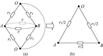
Figure 4. (a) shows a 1 × 2 apple surface network model, where two O nodes are connected by a wire to form a pole. (b) is its equivalent circuit, where r1 = r0/2. |
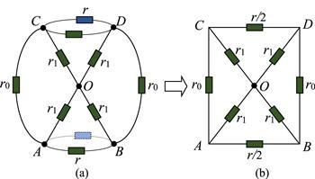
Figure 5. (a) is a 2 × 2 apple surface network model, (b) is its equivalent circuit, where r1 = r/2. |
The following uses the theoretical formula and the actual circuit calculation to compare and verify the correctness of the theoretical formula.
Firstly, their general formulas are given according to equations (5 ) and (6 ). When $\{{y}_{1},{y}_{2}\}\ne 0,$ taking m = 1 and n = 2 in equation (5 ), yielding6 ), yielding
$\begin{eqnarray}{R}_{1\times 2}\left({d}_{1},{d}_{2}\right)=2r\left(\displaystyle \frac{{F}_{2}^{(1)}-{g}_{{x}_{2},{x}_{1}}^{(1)}\cos \left({y}_{1}\pi \right)\cos \left({y}_{2}\pi \right)}{{\lambda }_{1}^{2}+{\bar{\lambda }}_{1}^{2}-2}\right).\end{eqnarray}$ 
When ${y}_{2}=0,$ taking m = 1 and n = 2 in equation ( $\begin{eqnarray}R\left({d}_{1},O\right)=r\displaystyle \frac{{F}_{2}^{(1)}}{{\lambda }_{1}^{2}+{\bar{\lambda }}_{1}^{2}-2}.\end{eqnarray}$ 
Since ${\theta }_{1}=i\pi /m,$ when m = 1,n = 2, it reduces to ${\theta }_{1}=\pi ,$ Substituting (2 ) and (3 ) to get
$\begin{eqnarray*}{\lambda }_{1}+{\bar{\lambda }}_{1}=2+4v,{g}_{0,0}^{(1)}={F}_{2}^{(1)}=2+4v,{g}_{0,1}^{(1)}=2{F}_{1}^{(1)}=2.\end{eqnarray*}$ 
Refer to node labeling in figure 4, when ${d}_{1}\left({x}_{1},{y}_{1}\right)=A\left(0,1\right),$ ${d}_{2}\left({x}_{2},{y}_{2}\right)=B\left(1,1\right),$ by (53 ) one gets
$\begin{eqnarray}\begin{array}{l}{R}_{1\times 2}\left(A,B\right)=2r\left(\displaystyle \frac{{F}_{2}^{(1)}-{g}_{1,0}^{(1)}}{{\lambda }_{1}^{2}+{\bar{\lambda }}_{1}^{2}-2}\right)\\ \,=\,r\left(\displaystyle \frac{2+4v-2}{8v\left(v+1\right)}\right)=\displaystyle \frac{r{r}_{0}}{2\left(r+{r}_{0}\right)}.\end{array}\end{eqnarray}$ 
When ${d}_{1}\left({x}_{1},{y}_{1}\right)=A\left(0,1\right),$ ${d}_{2}\left({x}_{2},{y}_{2}\right)=O\left(0,0\right),$ then by (54 ) one gets
$\begin{eqnarray}{R}_{1\times 2}\left(A,O\right)=r\displaystyle \frac{2+4v}{16v\left(v+1\right)}=\displaystyle \frac{{r}_{0}+2r}{8\left({r}_{0}+r\right)}{r}_{0}.\end{eqnarray}$ 
Next, according to the actual calculated equivalent circuit in figure 4, yielding
$\begin{eqnarray}{R}_{1\times 2}\left(A,B\right)={r}_{1}//\displaystyle \frac{r}{2}=\displaystyle \frac{{r}_{1}r}{2{r}_{1}+r}=\displaystyle \frac{{r}_{0}r}{2\left({r}_{0}+r\right)},\end{eqnarray}$ 
$\begin{eqnarray}{R}_{1\times 2}\left(A,O\right)=\displaystyle \frac{{r}_{1}}{2}//\left(\displaystyle \frac{{r}_{1}}{2}+\displaystyle \frac{r}{2}\right)=\displaystyle \frac{{r}_{0}\left({r}_{0}+2r\right)}{8\left({r}_{0}+r\right)}.\end{eqnarray}$ 
According to the above calculation, when m = 1 and n = 2, the correctness of theoretical formula (5 ) is verified by comparing equation (55 ) with (57 ), and the correctness of theoretical formula (6 ) is verified according to equations (56 ) and (58 ).
First we begin the theoretical calculation. When $\{{y}_{1},{y}_{2}\}\ne 0,$ taking m = 2 and n = 2 in equation (5 ), one can get6 ), one can get
$\begin{eqnarray}\begin{array}{l}{R}_{2\times 2}\left({d}_{1},{d}_{2}\right)=r\left(\displaystyle \frac{{F}_{2}^{(1)}\left({S}_{{y}_{1},1}^{2}+{S}_{{y}_{2},1}^{2}\right)-2{g}_{{x}_{2},{x}_{1}}^{(1)}{S}_{{y}_{1},1}{S}_{{y}_{2},1}}{{\lambda }_{1}^{2}+{\bar{\lambda }}_{1}^{2}-2}\right)\\ \,+\,r\left(\displaystyle \frac{{F}_{2}^{(2)}-{g}_{{x}_{2},{x}_{1}}^{(2)}\cos \left({y}_{1}\pi \right)\cos \left({y}_{2}\pi \right)}{{\lambda }_{2}^{2}+{\bar{\lambda }}_{2}^{2}-2}\right).\end{array}\end{eqnarray}$ 
When ${y}_{2}=0,$ taking m = 2 and n = 2 in equation ( $\begin{eqnarray}R\left({d}_{1},O\right)=r\displaystyle \frac{{F}_{2}^{(1)}{S}_{{y}_{1},1}^{2}}{{\lambda }_{1}^{2}+{\bar{\lambda }}_{1}^{2}-2}+r\displaystyle \frac{{F}_{2}^{(2)}}{2\left({\lambda }_{2}^{2}+{\bar{\lambda }}_{2}^{2}-2\right)}.\end{eqnarray}$ 
In addition, when m = 2, n = 2, we have ${\theta }_{1}=\pi /2,$ ${\theta }_{2}=\pi ,$ substituting to (2 ) and (3 ) to get
$\begin{eqnarray*}{\lambda }_{1}+{\bar{\lambda }}_{1}=2+2v,{\lambda }_{2}+{\bar{\lambda }}_{2}=2+4v,\end{eqnarray*}$ 
$\begin{eqnarray*}{g}_{0,0}^{\left(1\right)}={F}_{2}^{\left(1\right)}=2+2v,{g}_{0,1}^{\left(1\right)}=2{F}_{1}^{\left(1\right)}=2,\end{eqnarray*}$ 
$\begin{eqnarray*}{g}_{0,0}^{(2)}={F}_{2}^{(2)}=2+4v,{g}_{0,1}^{(2)}=2{F}_{1}^{(2)}=2.\end{eqnarray*}$ 
$\begin{eqnarray*}\begin{array}{l}{S}_{1,1}^{2}={\sin }^{2}\left(1-\displaystyle \frac{1}{2}\right)\displaystyle \frac{\pi }{2}=\displaystyle \frac{1}{2},{S}_{2,1}^{2}={\sin }^{2}\left(2-\displaystyle \frac{1}{2}\right)\displaystyle \frac{\pi }{2}=\displaystyle \frac{1}{2},\\ {S}_{1,2}^{2}={\sin }^{2}\left(1-\displaystyle \frac{1}{2}\right)\pi =1.\end{array}\end{eqnarray*}$ 
Refer to node labeling in figure 5, when ${d}_{1}\left({x}_{1},{y}_{1}\right)=A\left(0,1\right),$ ${d}_{2}\left({x}_{2},{y}_{2}\right)=B\left(1,1\right),$ by (59 ) one can get
$\begin{eqnarray}\begin{array}{l}{R}_{2\times 2}\left(A,B\right)=r\displaystyle \frac{{F}_{2}^{(1)}-{g}_{0,1}^{(1)}}{{\lambda }_{1}^{2}+{\bar{\lambda }}_{1}^{2}-2}\\ \,+\,r\displaystyle \frac{{F}_{2}^{(2)}-{g}_{0,1}^{(2)}}{{\lambda }_{2}^{2}+{\bar{\lambda }}_{2}^{2}-2}.\end{array}\end{eqnarray}$ 
If we simplify (61), we get $\begin{eqnarray}\begin{array}{l}{R}_{2\times 2}\left(A,B\right)=r\left(\displaystyle \frac{2v}{4\left(2+v\right)}+\displaystyle \frac{4v}{16\left(1+v\right)}\right)\\ \,=\,\displaystyle \frac{4+3v}{4\left(2+v\right)\left(1+v\right)}r.\end{array}\end{eqnarray}$ 
When ${d}_{1}({x}_{1},{y}_{1})=A(0,1),$ ${d}_{2}({x}_{2},{y}_{2})=C(0,2),$ then by (59 ) one can get
$\begin{eqnarray}\begin{array}{l}{R}_{2\times 2}\left(A,C\right)=r\left(\displaystyle \frac{{F}_{2}^{(1)}-{g}_{0,0}^{(1)}}{{\lambda }_{1}^{2}+{\bar{\lambda }}_{1}^{2}-2}\right)\\ \,\,+\,r\left(\displaystyle \frac{{F}_{2}^{(2)}+{g}_{0,0}^{(2)}}{{\lambda }_{2}^{2}+{\bar{\lambda }}_{2}^{2}-2}\right).\end{array}\end{eqnarray}$ 
If we simplify (63 ), we get
$\begin{eqnarray}\begin{array}{l}{R}_{2\times 2}\left(A,C\right)=r\left(\displaystyle \frac{2{F}_{2}^{(2)}}{{\lambda }_{2}^{2}+{\bar{\lambda }}_{2}^{2}-2}\right)\\ \,=\,r\displaystyle \frac{\left(2+4v\right)}{8v\left(1+v\right)}=\displaystyle \frac{1+2v}{4\left(1+v\right)}{r}_{0}.\end{array}\end{eqnarray}$ 
When ${d}_{1}({x}_{1},{y}_{1})=A(0,1),$ ${d}_{2}({x}_{2},{y}_{2})=D(1,2),$ then by (59 ) one can get65 ), we get
$\begin{eqnarray}{R}_{2\times 2}\left(A,D\right)=r\left(\displaystyle \frac{{F}_{2}^{(1)}-{g}_{0,1}^{(1)}}{{\lambda }_{1}^{2}+{\bar{\lambda }}_{1}^{2}-2}\right)+r\left(\displaystyle \frac{{F}_{2}^{(2)}+{g}_{0,1}^{(2)}}{{\lambda }_{2}^{2}+{\bar{\lambda }}_{2}^{2}-2}\right).\end{eqnarray}$ 
If we simplify ( $\begin{eqnarray}\begin{array}{l}{R}_{2\times 2}\left(A,D\right)=r\displaystyle \frac{2v}{4v\left(2+v\right)}\\ \,+\,r\displaystyle \frac{4+4v}{16v\left(1+v\right)}=\displaystyle \frac{2+3v}{4\left(2+v\right)}r.\end{array}\end{eqnarray}$ 
When ${d}_{1}\left({x}_{1},{y}_{1}\right)=A\left(0,1\right),$ ${d}_{2}\left({x}_{2},{y}_{2}\right)=O\left(0,0\right),$ then by (60 ) one can get
$\begin{eqnarray}R\left(A,O\right)=\displaystyle \frac{r}{2}\left(\displaystyle \frac{{F}_{2}^{(1)}}{{\lambda }_{1}^{2}+{\bar{\lambda }}_{1}^{2}-2}+\displaystyle \frac{{F}_{2}^{(2)}}{{\lambda }_{2}^{2}+{\bar{\lambda }}_{2}^{2}-2}\right).\end{eqnarray}$ 
Simplifying it to get $\begin{eqnarray}\begin{array}{l}R\left(A,O\right)=\displaystyle \frac{r}{2}\left(\displaystyle \frac{2+2v}{4v\left(2+v\right)}+\displaystyle \frac{2+4v}{16v\left(1+v\right)}\right)\\ \,=\,\displaystyle \frac{\left(3+2v\right)\left(2+3v\right)}{16\left(2+v\right)\left(1+v\right)}{r}_{0}.\end{array}\end{eqnarray}$ 
From above, equivalent resistances of $R(A,B),$ $R(A,C),$ $R(A,D)$ and $R(A,O)$ are calculated in terms of the theoretical formula. However, the resistance value calculated by the actual circuit in figure 5 is exactly the same as the theoretical value above, which once again verifies the correctness of the theoretical formula.
Case-3. When considering two nodes of ${d}_{1}({x}_{1},{y}_{1})$ and ${d}_{2}({x}_{1},{y}_{2}),$ and $\{{y}_{1},{y}_{2}\}\ne 0,$ from (5 ), the resistance formula of the $m\times n$ apple surface network can be written as2 ).
$\begin{eqnarray}\begin{array}{l}{R}_{m\times n}\left({d}_{1},{d}_{2}\right)=\displaystyle \frac{2r}{m}\left(\displaystyle \sum _{i=1}^{m-1}\displaystyle \frac{{F}_{n}^{(i)}}{{\lambda }_{i}^{n}+{\bar{\lambda }}_{i}^{n}-2}{\left({S}_{{y}_{1},i}-{S}_{{y}_{2},i}\right)}^{2}\right)\\ \,\,+\,\displaystyle \frac{2r}{m}\left(\displaystyle \frac{\left[1-\,\cos \left({y}_{1}\pi \right)\cos \left({y}_{2}\pi \right)\right]}{{\lambda }_{m}^{n}+{\bar{\lambda }}_{m}^{n}-2}{F}_{n}^{(m)}\right),\end{array}\end{eqnarray}$ 
where ${F}_{k}^{(i)}$ is defined in equation (Case-4. When considering two nodes of ${d}_{1}({x}_{1},{y}_{1})$ and ${d}_{2}({x}_{2},{y}_{1}),$ from (5 ), the resistance formula of the $m\times n$ apple surface network can be written as
$\begin{eqnarray}\begin{array}{l}{R}_{m\times n}\left({d}_{1},{d}_{2}\right)=\displaystyle \frac{4r}{m}\left(\displaystyle \sum _{i=1}^{m-1}\displaystyle \frac{{F}_{n}^{(i)}-{g}_{{x}_{2},{x}_{1}}^{(i)}}{{\lambda }_{i}^{n}+{\bar{\lambda }}_{i}^{n}-2}{S}_{{y}_{1},i}^{2}\right)\\ \,+\,\displaystyle \frac{2r}{m}\left(\displaystyle \frac{{F}_{n}^{(m)}-{g}_{{x}_{2},{x}_{1}}^{(m)}}{{\lambda }_{m}^{n}+{\bar{\lambda }}_{m}^{n}-2}\right),\end{array}\end{eqnarray}$ 
where ${g}_{{x}_{s},x}^{(i)}$ and ${F}_{k}^{(i)}$ are defined in (2).5. Visualization of potential function
The analytical expressions (1 ) and (4 ) of the potential function are accurate and concise, but they are quite abstract. In order to facilitate readers to understand its potential characteristics, we use Matlab drawing tool to plot the visual graph of potential functions (1 ) and (4 ). These figures can reveal the basic law of potential distribution. We consider the (m, n) = (60, 80) apple surface network. Take $r=20$ in all graphs, and take $v=\{1,2\}$, respectively, for comparison, where v = r/r0.
The parameters in figure 6 are designed as r = 20, ${d}_{1}({x}_{1},{y}_{1})={d}_{1}(0,20)$ and ${d}_{2}({x}_{2},{y}_{2})=O(0,0),$ where the parameter v = 1 in figure 6(a) is different from the parameter v = 2 in figure 6(b). Since $U(0,0)=0$ is assumed, it causes all the potential values to be $U(x,y)\geqslant 0.$ Two images show two potential maxima at positions (0, 20) and (80, 20). The two maximum potential values in the figure are given by the theoretical function, which are completely consistent with the actual situation. For example, we analyze the actual circuit. Since $U({x}_{2},{y}_{2})=U(0,0)=0$ and cycle, it leads to $U(x,0)=U(x,60)=0.$ Since ${d}_{1}({x}_{1},{y}_{1})={d}_{1}(0,20)$ is the input point of current, the potential of this node must be the highest point. Due to the cycle, nodes $d(0,20)$ and $d(80,20)$ overlap at the same point on the apple surface network, but figure 6 divides nodes $d(0,20)$ and $d(80,20)$ into two positions, so there are two peaks in the coordinate diagram. Obviously, the potential distribution of the actual circuit is exactly the same as that of the viewable potential.
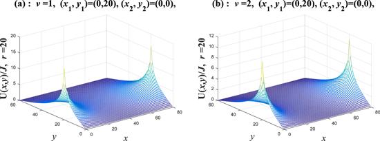
Figure 6. Potential function diagram plotted based on equation ( |
The parameters in figure 7 are designed as r = 20, ${d}_{1}({x}_{1},{y}_{1})={d}_{1}(4,20)$ and ${d}_{2}({x}_{2},{y}_{2})=O(0,0),$ where the parameter v = 1 in figure 7(a) is different from the parameter v = 2 in figure 7(b). Since $U(0,0)=0$ is assumed, it causes all the potential values to be $U(x,y)\geqslant 0.$ Two images show a maximum potential value at position (4, 20). We analyze the actual circuit, since $U\left({x}_{2},{y}_{2}\right)$ = $U(0,0)=0$ and cycle, it leads to $U\left(x,0\right)=U\left(x,60\right)=0.$ Since ${d}_{1}({x}_{1},{y}_{1})\,={d}_{1}(40,20)$ is the input point of current, the potential of this node must be the highest point. Obviously, the potential distribution of the actual circuit is exactly the same as that of the viewable potential.
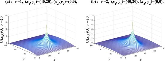
Figure 7. Potential function diagram plotted based on equation ( |
The parameters in figure 8 are designed as r = 20, ${d}_{1}(0,30)$ and ${d}_{2}(50,30),$ where the parameter v = 1 in figure 8(a) is different from the parameter v = 2 in figure 8(b). Since $U(0,0)=0$ is assumed, there is a maximum value at the current input point ${d}_{1}(0,30)$ and a minimum value at the current output point ${d}_{2}(50,30).$ For example, we analyzed the actual circuit. Due to the cyclical nature, nodes $d(0,30)$ and $d(80,30)$ coincide at the same point on the apple surface network, while nodes $d(0,30)$ and $d(80,30)$ are separated in figure 8, so there are two peaks in the coordinate diagram. Obviously, the potential distribution of the actual circuit is exactly the same as the viewable potential plotted according to the theoretical function.
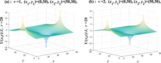
Figure 8. Potential function diagram plotted based on equation ( |
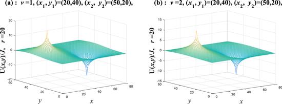
The parameters in figure 9 are designed as $r=20,$ ${d}_{1}(20,40)$ and ${d}_{2}(50,20),$ where the parameter v = 1 in figure 9(a) is different from the parameter v = 2 in figure 9(b). Since $U(0,0)=0$ is assumed, there is a maximum value at the current input point ${d}_{1}(20,40)$ and a minimum value at the current output point ${d}_{2}(50,20).$ It is obvious that the actual circuit potential distribution in these cases is exactly the same as the viewable potential plotted according to the theoretical function.
Figure 9. Potential function diagram plotted based on equation ( |
6. Comment
Investigation shows that the circuit network model has important application value in many disciplines, and many complex problems can be simulated by establishing the network model. However, it is important and difficult to find an explicit solution of the potential function in an arbitrary m × n resistor network. The arbitrary m × n apple surface network in figure 1 is a new type of model that has not been studied before. This paper obtained two general and exact potential functions of an arbitrary m × n apple surface network by the RT-V method. At the same time, two equivalent resistance analytic expressions are derived for the first time. A series of theoretical results derived in this paper establishes the new theoretical basis for future research of related disciplines. The network of figure 1 has a pair of special boundary resistors of r1, which is different from other resistors on the longitude line and leads to the difficulty of research. The key breakthrough point of this paper is the derivation of equations (20 ) and (21 ). Since the results are abstract, in order to verify the correctness of the theory, we use 1 × 2 and 2 × 2 circuits to compare and verify the correctness of the theoretical formula. These verification procedures also help readers to further understand the arbitrary m × n resistor network. At the end of this paper, the eight visual images of potential function in various cases are given, and the difference of potential function in different cases of $v=1$ and 2 is compared ($v=r/{r}_{0}$). These visual images are helpful to strengthen readers’ understanding of the characteristics of potential function.
Compared with the study in reference [51], there are three significant differences. The first is that the resistance arrangement in the network is different; the second is that the matrix elements and their matrix transformation are different; the third is that the conclusion of the electrical characteristics is different (this paper needs to use two formulas to express the results, while reference [51] only uses one formula to express the results).