Welcome to visit Communications in Theoretical Physics,
Mathematical Physics

Impact of asymmetric activity on interactions between information diffusion and disease transmission in multiplex networks

  • Xiaoxiao Xie ,
  • Liang’an Huo , ,
  • Laijun Zhao ,
  • Ying Qian
Expand
  • Business School, University of Shanghai for Science and Technology, Shanghai 200093, China

Author to whom any correspondence should be addressed.

Received date: 2022-11-24

  Revised date: 2023-02-23

  Accepted date: 2023-04-19

  Online published: 2023-06-22

Copyright

© 2023 Institute of Theoretical Physics CAS, Chinese Physical Society and IOP Publishing

Abstract

Disease is a serious threat to human society. Understanding the characteristics of disease transmission is helpful for people to effectively control disease. In real life, it is natural to take various measures when people are aware of disease. In this paper, a novel coupled model considering asymmetric activity is proposed to describe the interactions between information diffusion and disease transmission in multiplex networks. Then, the critical threshold for disease transmission is derived by using the micro-Markov chain method. Finally, the theoretical results are verified by numerical simulations. The results show that reducing the activity level of individuals in the physical contact layer will have a continuous impact on reducing the disease outbreak threshold and suppressing the disease. In addition, the activity level of individuals in the virtual network has little impact on the transmission of the disease. Meanwhile, when individuals are aware of more disease-related information, the higher their awareness of prevention will be, which can effectively inhibit the transmission of disease. Our research results can provide a useful reference for the control of disease transmission.

Cite this article

Xiaoxiao Xie , Liang’an Huo , Laijun Zhao , Ying Qian . Impact of asymmetric activity on interactions between information diffusion and disease transmission in multiplex networks[J]. Communications in Theoretical Physics, 2023 , 75(7) : 075001 . DOI: 10.1088/1572-9494/acce31

1. Introduction

Diseases are a serious threat to human society, for example, COVID-19, tuberculosis and influenza may cause many disasters to public security and individuals’ health [1]. How to prevent and control diseases effectively has become an important and urgent problem in the field of public health, it is of great practical significance to analyze the transmission of diseases. In this regard, the modeling of disease transmission has attracted great attention in different research fields [2, 3].
The study of disease transmission has a long history, dating back to the early 20th century [4, 5]. In 1927, the famous ‘compartment model’ was established by Kermack and McKendrick, and then the theoretical threshold of disease transmission was obtained [6]. In the following decades, almost all relevant studies have cited the core hypothesis of the compartment model, that is, assuming that individuals are evenly mixed in space. After that, some classical mathematical models such as $\mathrm{SIS}$ (susceptible–infected–susceptible) model and $\mathrm{SIR}$ (susceptible– infected–recovered) model have laid the foundation in the field of disease transmission [7, 8]. Based on these classical disease transmission models, a terrific amount of work has been completed to explore the characteristics of disease transmission. At the end of the 20th century, small-world networks and scale-free networks have been widely studied [9], which initiated a new perspective on disease transmission [10, 11]. It has been found that the framework of complex networks can be used to describe many real systems [12, 13]. A tremendous amount of research works on transmission dynamics have been gained under the framework of complex networks [14, 15]. Buono et al studied a $\mathrm{SIR}$ disease transmission model in a partially overlapped multiplex network consisting of two layers that share a fraction q of nodes, and they found that vaccination or isolation of only the layer with higher propagation capacity can greatly reduce the total branching factor of the network [16]. Alvarez-Zuzek et al studied disease transmission in multiplex networks by opinion exchanges on vaccination, which concludes that the exchange of views among individuals had an impact on the vaccination rate [17]. Sartori et al explored the effectiveness of vaccination by comparing the vaccination strategies of seven nodes in twelve real-world complex networks [18]. Cremonini et al proposed a new agent group dynamic model of network transmission to study the dynamics of disease transmission [19]. Silva et al studied two rules of disease transmission in heterogeneous networks, and the results showed that strategies that improve the perception of who is socially very active can improve the mitigation of disease outbreaks [20]. Jin et al deeply discussed the dynamics of the disease transmission process in a physical contact network and proposed a cascade fault model with load distribution parameters and a disease $\mathrm{SIR}$ model [21].
Individual awareness influences individual behavior [22, 23]. In real life, once people realize the potential threat of disease, they will take effective measures to prevent infection in time, such as wearing masks, vaccination, etc. The awareness is reflected in the contact behavior that would change the connection patterns [24, 25]. Therefore, scholars have begun to study the transmission dynamics of information and disease on multiple networks [26]. For example, Funk et al introduced the effect of disease-relevant awareness in the research of disease transmission, which indicates that disease-relevant awareness was able to moderate the scale of the infectious disease [27]. Granell et al analyzed a coupled dynamical process of awareness and disease on the top of multiplex networks and found that the critical threshold of disease transmission was determined by the dynamics of awareness and the topology of the virtual networks [28]. Chen et al introduced the inter-layer mutual recognition mechanism into the dynamics of information disease interaction on multiple networks. The research results show that individuals clearly disclosing their infection and awareness status to neighbors, especially those who have real contacts, is helpful in suppressing disease spread [29]. Silva et al proposed a mathematical model of the transmission of diseases related to awareness in a complex network and verified that the velocity characterizing the diffusion of awareness greatly influences the disease prevalence [30]. Wang et al used real data to investigate the coevolutionary mechanism and dynamics between information diffusion and disease transmission in multiple networks, which proves that there was asymmetric interaction between information diffusion and disease transmission dynamics [31]. Pan et al investigated the coupled awareness-disease dynamics in multiplex networks considering individual heterogeneity, indicating that local and global information can only reduce the prevalence of disease [32].
Different individuals have different levels of activity, which will affect individual behavior. In previous studies, the level of individual activity was considered as the degree of contact between individuals in the process of disease transmission. Due to the heterogeneity of individuals, each individual in the network will have two states (active or inactive). Active individuals are infected with a certain probability by contacting infected neighbors; inactive individuals will not contact other individuals because of their self-protection status, and will not participate in the process of disease transmission - a process known as the interaction between individuals. Kotnis et al investigated the impact of individual activity on disease transmission and proved that only controlling the activity level of infected individuals can effectively inhibit the transmission of the disease [33]. Rizzo et al proposed an activity-driven model of dynamical networks to study the factors influencing disease transmission [34]. Based on the $\mathrm{SIR}$ (Susceptible-Infected-Removed) model, Liu et al investigated the impact of individual activity on transmission dynamics of complex networks, and the results showed that the critical threshold of disease transmission was increased by node activity [35]. Fan et al studied the two interacting processes of information awareness and disease transmission on the same individual who has a different behavior status on the multiplex networks, which indicates that individual activity had a significant impact on the threshold of disease transmission [36].
However, the level of activity is not a fixed characteristic of individuals and will change with the change in environment. Therefore, individuals have different levels of activity in the information transmission layer and the disease transmission layer. For example, some people are active in the virtual world and like to release information online, but they are not active in the real world; some older people are just more active in real life, but they do not often surf the Internet. Therefore, it is worthwhile to study the impact of individual asymmetric activities on the dynamic transmission process of disease in multiple networks. Different from previous studies on the impact of individual activity on the transmission of disease, in this paper, asymmetric activity is introduced into the classical $\mathrm{UAU}\unicode{x02013}\mathrm{SIS}$ (Unaware-Aware-Unaware-Susceptible-Infected-Susceptible) model. In the information diffusion layer, during each time step, an active individual interacts with all their neighbors, while an inactive individual can only interact with their active neighbors. However, at the disease transmission level, an individual is at risk of becoming infected once he or she contacts an infected neighbor, whether he or she is active or not. Then, the critical threshold for disease transmission of the coupled model is calculated by using the micro-Markov chain method. Finally, the theoretical results are verified by numerical simulations.
The remaining sections of this paper are organized as follows. Firstly, the model-related assumptions are introduced in detail. In addition, the micro-Markov chain method is used to analyze the model and drive the analytical expression of the disease threshold in section 3. Secondly, in section 4, numerical simulations are performed to validate theoretical predictions. Finally, we conclude the paper and perform some outlooks in section 5.

2. The model-related assumptions

Previous scholars have proposed that individuals have the same level of activity in multiplex networks [36]. In fact, an individual’s personality and living environment will lead to different levels of activity in different environments. Here, a novel model considering asymmetric activity is proposed based on the $\mathrm{UAU}\unicode{x02013}\mathrm{SIS}$ model proposed by Granell et al [28]. In order to better describe the model, we give the following assumptions:

Network structure assumption. As shown in figure 1, our model is implemented on a multiplex network. To illustrate it, we construct a two-layer network, which is used to describe the diffusion of disease-related information on the social networks layer and the transmission of diseases in the physical contact layer, respectively. For simplicity, we assume that the multiplex network is unweighted and undirected. The relationship between the two layers is a coupling dynamic process of disease transmission and information diffusion. A virtual connection between two-layer networks means that the mapping relationship of node pairs, and the individuals in the two-layer networks are represented by circles. The upper layer stands for the disease-related information diffusion on social networks (e.g., Twitter, Facebook and WeChat) denoted by the $\mathrm{UAU}$ (unaware-aware-unaware) layer. The nodes are divided into two states: unaware (${\rm{U}}$) and (${\rm{A}}$) aware. State ${\rm{U}}$ indicates that the individuals are not aware of disease-related information; state ${\rm{A}}$ indicates that individuals are aware of the disease-related information. It is worth noting that, on the one hand, individuals who are not aware of the existence of the disease will not take any measures to avoid being infected by the disease; on the other hand, individuals who are aware of the existence of the disease will diffuse disease-related information to their neighbors and take measures to avoid being infected by the disease. Among them, if an unaware individual contacts an aware neighbor, he or she will acquire the disease-related information with a probability $\lambda .$ Furthermore, an aware individual will forget the disease-related information with the probability $\delta .$

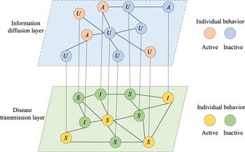
Figure 1. Schematic diagram of the coupled $\mathrm{UAU}\unicode{x02013}\mathrm{SIS}$ model multiple networks. The upper layer is the virtual information layer, where nodes have two possible states: aware ($A$) and unaware ($U$); The lower layer network denotes the physical contact layer, where nodes also have two possible states: susceptible ($S$) and infected ($I$). For the activity behavior of nodes, the orange and blue dots represent the active and inactive status of nodes in the virtual information layer, respectively. Meanwhile, the yellow and green dots denote the active and inactive status of nodes in the physical contact layer, respectively.
The mechanisms of disease transmission and information diffusion are similar but are not identical completely. Individuals have subjective initiative. In the process of disease transmission, even if individuals take various preventive measures and are unwilling to be infected by the disease, it is still accompanied by the risk of being infected by the disease. In the diffusion of information, different types of edges not only have different diffusion power but also have different diffusion modes, the contact intensity in disease transmission will only cause the difference in transmission probability. The lower layer denotes the transmission of disease in the physical contact network (such as the mutual contact relationship in daily life) by using the classical $\mathrm{SIS}$ (susceptible-infected-susceptible) model. The nodes are divided into two states: susceptible and infected. Susceptible individuals (${\rm{S}}$) represent healthy individuals, which may be infected by neighbor individuals. Infected individuals (${\rm{I}}$) denote individuals who have been infected and will infect their neighbors. Among them, a susceptible individual would transmit an infection through one contact with an infected neighbor at the basic rate $\beta ;$ meanwhile, an infected individual will spontaneously recover with the probability $\mu .$ In addition, if individuals know disease-related information and take effective preventive measures in time, the probability of infection will be reduced. Therefore, $\phi $ is represented as an information reduction factor. We use ${\beta }^{A}$ and ${\beta }^{U}$ to represent the infection rate of individuals who are aware of disease information and unaware of disease information, respectively, and we have ${\beta }^{A}=\phi {\beta }^{U}=\phi \beta .$

Assumption of individual disease infection rate. In particular, the mapping pattern between the corresponding nodes in the two-layer network is one-to-one, that is, an individual is assumed to appear in the social network and the physical contact network at the same time. As proposed in [37, 38], in the layer of disease transmission, the disease infection rate depends on the ‘susceptibility’ of susceptible individuals and the ‘transmission ability’ of infected individuals, which can be defined as:

$\begin{eqnarray}{M}_{ij}=\left\{\begin{array}{cc}{E}_{i}{T}_{j}, & {\rm{i}}\,{\rm{is}}\,{\rm{susceptible}}\,{\rm{and}}\,{\rm{j}}\,{\rm{is}}\,{\rm{infectious}};\\ {T}_{i}{E}_{j}, & {\rm{i}}\,{\rm{is}}\,{\rm{infectious}}\,{\rm{and}}\,{\rm{j}}\,{\rm{is}}\,{\rm{susceptible}};\\ 0, & {\rm{otherwise}}.\end{array}\right.\end{eqnarray}$
${M}_{ij}$ represents the true probability of an individual being infected by the disease. As shown in the above equation (1), it mainly consists of two parts. ${E}_{i}$ refers to the susceptibility of susceptible individuals ($S$), which indicates the probability that susceptible individual $i$ will be infected through one contact with an infected individual. In this paper, individual susceptibility is mainly affected by the activity $\omega $ of individuals. The more active an individual is, the stronger his susceptibility is, we give ${E}_{i}=\omega ;$ ${T}_{i}$ refers to the transmission ability of infected individuals ($I$), which indicates the transmission rate that the individual would transmit an infection through one contact with a susceptible individual, we give ${T}_{j}=\beta .$ Therefore, based on assumption 1, the true probability of being infected by the disease after an individual contacts an infected neighbor is ${M}_{j}=\omega \beta .$ In real life, when individuals know the disease-related information, they will take a series of preventive measures, so the probability of being infected by the disease will be lower. Therefore, the real probability of infection of individuals in state $A$ is obtained as $\omega {\beta }^{A}$, and the real probability of infection of individuals in state $U$ is obtained as $\omega {\beta }^{U}$, where ${\beta }^{A}=\phi {\beta }^{U},$ $\phi $ is the infection reduction factor when a susceptible individual is aware of the disease. When individuals are aware of disease-related information, they will take appropriate measures to prevent disease.

Assumption of asymmetric activity. Here, heterogeneous activity is used to describe the activity of individuals. Inactive individuals do not take the initiative to contact and generate connection edges in the network, and most of them wait for active nodes to activate and generate connection edges to connect to them. The individual in the proposed model will be involved in the diffusion of information and the transmission of diseases. Individuals have different levels of activity in different environments. The activity of the information transmission layer refers to whether individuals actively diffuse disease-related information; during each time step, an active individual interacts with all its neighbors, while an inactive node can only be interacted with by its active neighbors. The activity of the disease transmission layer denotes some behavioral characteristics of individuals (for example running around during the disease and going out without masks). Individuals, whether active or not, are at risk of becoming infected once they contact with infected neighbors.

Assumption of key parameters of the model. In order to introduce the proposed model more clearly, we first make assumptions about the definition of key quantities or parameters in the model in table 1.

3. The analytical results based on mean-field method

It is well known that infectious disease thresholds are important parameters for preventing and controlling the spread of disease. In this section, we conduct a theoretical analysis of our model to derive the critical threshold of disease transmission by using the mean-field method.
Table 1. Definition of some key quantities or parameters in the proposed disease model.
Symbol Definition
$\lambda $ The probability that unaware individuals can communicate with aware individuals to obtain information.
$\delta $ The probability that an aware individual forgets information
$\beta $ The probability that the susceptible individual would transmit an infection through one contact with an infected neighbor.
$\mu $ The probability that an infected individual recovering to a susceptible state
$\alpha $ The activity level of individuals in the information diffusion layer
$\omega $ The activity level of individuals in the disease transmission layer
${\beta }^{U}$ The probability that an unaware susceptible individual is infected by one of his infected neighbors
${\beta }^{A}$ The probability that an aware susceptible individual is infected by one of his infected neighbors
$\phi $ Infection reduction factor when a susceptible individual is aware of the disease.
${r}_{i}$ The probability that an individual will not be informed
${q}_{i}^{U}$ The probability that an individual who is not aware of the existence of the disease information will not be infected
${q}_{i}^{A}$ The probability that an individual who is aware of the existence of the disease information will be infected
There exists four possible states for any node pair in the current model, which include unaware susceptible ($US$), unaware infected ($UI$), aware susceptible ($AS$), and aware infected ($AI$). Generally, it is assumed that an infected individual is certainly aware of the disease and thus the $UI$ state is nonexistent. And twelve sub-states: ${U}^{m}{S}^{a},$ ${U}^{m}{S}^{d},$ ${A}^{m}{S}^{a},$ ${A}^{m}{S}^{d},$ ${A}^{m}{I}^{a},$ ${A}^{m}{I}^{d},$ ${U}^{n}{S}^{a},$ ${U}^{n}{S}^{d},$ ${A}^{n}{S}^{a},$ ${A}^{n}{S}^{d},$ ${A}^{n}{I}^{a},$ ${A}^{n}{I}^{d},$ the superscript sign $m$ and $n$ represent the active and inactive states of individuals in the upper layer network, respectively. Similarly, superscript $a$ and $d$ denote the active state and inactive state of individuals in the lower layer network, respectively. In addition, any one of the 12 sub-states can be transformed into other possible ones with a certain probability, and the corresponding state transition is shown in figures 2 and 3.
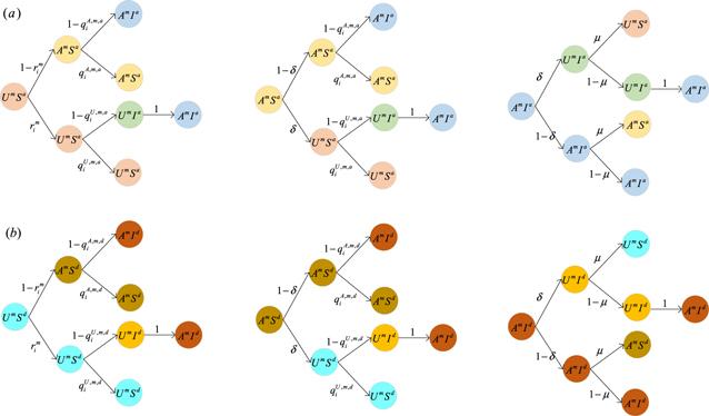
Figure 2. Transition probability trees for three active states in the information diffusion layer per time step. (a) represents the state probability tree of nodes that are active in the disease transmission layer; (b) denotes the state probability tree of nodes that are inactive in the disease transmission layer. Nodes that are active in the information diffusion layer and active in the disease transmission layer aware of disease will not be infected with probability ${q}_{i}^{A,m,a};$ nodes that are active in the information diffusion layer and inactive in the disease transmission layer aware of disease will not be infected with probability ${q}_{i}^{A,m,d};$ nodes that are active in the information diffusion layer and active in the disease transmission layer unaware of disease will not be infected with probability ${q}_{i}^{U,m,a};$ nodes that are active in the information diffusion layer and inactive in the disease transmission layer unaware of disease will not be infected with probability ${q}_{i}^{U,m,d}.$ ${r}_{i}^{m}$ is used to denote the probability that nodes that are active in the information diffusion layer will not be informed by any neighbors who are aware of the disease. $\delta $ is the probability that nodes are aware of the information of disease but may forget, and $\mu $ is the probability that infectious individuals may recover.
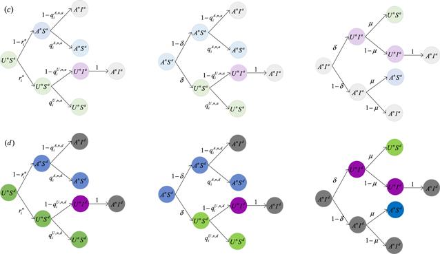
Figure 3. Transition probability trees for three inactive states in the information diffusion layer per time step. (c) represents the state probability tree of nodes that are active in the disease transmission layer; (d) denotes the state probability tree of nodes that are inactive in the disease transmission layer. Nodes that are inactive in the information diffusion layer and active in the disease transmission layer aware of disease will not be infected with probability ${q}_{i}^{A,n,a};$ nodes that are active in the information diffusion layer and inactive in the disease transmission layer aware of disease will not be infected with probability ${q}_{i}^{A,n,d};$ nodes that are inactive in the information diffusion layer and inactive in the disease transmission layer unaware of disease will not be infected with probability ${q}_{i}^{U,n,a};$ nodes that are inactive in the information diffusion layer and inactive in the disease transmission layer unaware of disease will not be infected with probability ${q}_{i}^{U,n,d}.$ ${r}_{i}^{n}$ is used to denote the probability that nodes that are inactive in the information diffusion layer will not be informed by any neighbors who are aware of the disease.
Then, the reaction process of the multiplex networks model can be schematically represented by:

(1)Behavior state change in the upper layer network

$\begin{eqnarray*}{U}^{m}\mathop{\longrightarrow }\limits^{1-\alpha }{U}^{n},{U}^{n}\mathop{\longrightarrow }\limits^{\alpha }{U}^{m};\end{eqnarray*}$
$\begin{eqnarray*}{A}^{m}\mathop{\longrightarrow }\limits^{1-\alpha }{A}^{n},{A}^{n}\mathop{\longrightarrow }\limits^{\alpha }{A}^{m}.\end{eqnarray*}$

(2)Behavior state change in the lower layer network

$\begin{eqnarray*}{S}^{a}\mathop{\longrightarrow }\limits^{1-\omega }{S}^{d},{S}^{d}\mathop{\longrightarrow }\limits^{\omega }{S}^{a};\end{eqnarray*}$
$\begin{eqnarray*}{I}^{a}\mathop{\longrightarrow }\limits^{1-\omega }{I}^{d},{I}^{d}\mathop{\longrightarrow }\limits^{\omega }{I}^{a}.\end{eqnarray*}$

(3)Active spreading in the upper layer network

$\begin{eqnarray*}{U}^{m}S+AS\mathop{\longrightarrow }\limits^{\lambda }{A}^{m}S+AS,{U}^{m}S+AI\mathop{\longrightarrow }\limits^{\lambda }{A}^{m}S+AI.\end{eqnarray*}$

(4)Inactive spreading in the upper layer network

$\begin{eqnarray*}{U}^{n}S+{A}^{m}S\mathop{\longrightarrow }\limits^{\lambda }{A}^{n}S+{A}^{m}S,{U}^{n}S+{A}^{m}I\mathop{\longrightarrow }\limits^{\lambda }{A}^{n}S+{A}^{m}I.\end{eqnarray*}$

(5)Active spreading in the lower layer network

$\begin{eqnarray*}\begin{array}{l}U{S}^{m}+AI\mathop{\longrightarrow }\limits^{{\beta }^{u}}U{I}^{m}+AI\mathop{\longrightarrow }\limits^{1}A{I}^{m}\\ \,+\,AI,A{S}^{m}+AI\mathop{\longrightarrow }\limits^{{\beta }^{A}}A{I}^{m}+AI.\end{array}\end{eqnarray*}$

(6)Inactive spreading in the lower layer network

$\begin{eqnarray*}\begin{array}{l}U{S}^{n}+A{I}^{m}\mathop{\longrightarrow }\limits^{\omega {\beta }^{u}}U{I}^{n}+A{I}^{m}\mathop{\longrightarrow }\limits^{1}A{I}^{n}+A{I}^{m},\\ A{S}^{n}+A{I}^{m}\mathop{\longrightarrow }\limits^{\omega {\beta }^{A}}A{I}^{n}+A{I}^{m}.\end{array}\end{eqnarray*}$

(7)Recoveries

$\begin{eqnarray*}AS\mathop{\longrightarrow }\limits^{\delta }US,AI\mathop{\longrightarrow }\limits^{\mu }AS.\end{eqnarray*}$
On the information diffusion layer, ${r}_{i}$ is represented as the total probability that node $i$ is not informed, consisting of two parts, where ${r}_{i}^{m}$ is the probability that an active node $i$ is not informed at time step $t$ and ${r}_{i}^{n}$ is denoted as the probability that an inactive node $i$ is not informed at time step $t.$ On the disease transmission layer, ${q}_{i}^{U}$ is denoted as the total probability that the unaware-state node $i$ is not infected by contacting neighbors, which is composed of two parts, the first part is ${q}_{i}^{U,m},$ indicating the probability that the active node is not infected; the second part is ${q}_{i}^{U,n},$ indicating the probability that the inactive node is not infected. Similarly, we can deduce that ${q}_{i}^{A}$ also consists of two parts ${q}_{i}^{A,m}$ and ${q}_{i}^{A,n}.$ Based on the above, we have ${r}_{i}=\alpha {r}_{i}^{m}+(1-\alpha ){r}_{i}^{n},$ ${q}_{i}^{A}\,=\omega {q}_{i}^{A,a}+(1-\omega ){q}_{i}^{A,d}$ and ${q}_{i}^{U}=\omega {q}_{i}^{U,a}+\left(1-\omega \right){q}_{i}^{U,d}.$
Considering the different activities of individuals in the upper and lower levels, We have ${q}_{i}^{A,m,a},$ ${q}_{i}^{A,m,d},$ ${q}_{i}^{U,m,a},$ ${q}_{i}^{U,m,d},$ ${q}_{i}^{A,n,a},$ ${q}_{i}^{U,n,a},$ ${q}_{i}^{A,n,a},$, ${q}_{i}^{A,n,d},$ ${q}_{i}^{U,n,d}.$ According to the above definitions, one can construct these probability trees of state in the proposed model as shown in figures 2 and 3.
In order to give a mean-field analysis, all nodes in the multiplexing network need to be divided into different categories according to the degree of nodes. $N(k,l)$ represents the number of nodes with degree $k$ in the information diffusion layer and degree $l$ in the disease transmission layer. The number of the three primary states at time $t$ is represented as $US\left(k,l,t\right),$ $AS\left(k,l,t\right),$ $AI\left(k,l,t\right),$ and ${\rho }^{US}\left(k,l,t\right),$ ${\rho }^{AS}\left(k,l,t\right)$ ${\rho }^{AI}\left(k,l,t\right)$ denotes the corresponding density, respectively. For example, ${\rho }^{US}\left(k,l,t\right)=\displaystyle \frac{US\left(k,l,t\right)}{N\left(k,l\right)}.$ Furthermore, condition ${\rho }^{US}\left(k,l,t\right)+{\rho }^{AS}\left(k,l,t\right)+{\rho }^{AI}\left(k,l,t\right)=1$ must be satisfied for each node $i.$
Given that node $i$ has $g\left(g\leqslant k\right)$ aware neighbors and $h\left(h\leqslant l\right)$ infected neighbors at time $t.$ The probability of node $i$ to stay in the unaware state is ${\left(1-\lambda {\rm{\Delta }}t\right)}^{g};$ the probability of node $i$ to stay in the aware susceptible state is ${\left(1-\omega {\beta }^{A}{\rm{\Delta }}t\right)}^{h};$ the probability of node $i$ to stay in the unaware susceptible state is ${\left(1-\omega {\beta }^{U}{\rm{\Delta }}t\right)}^{h}.$ Then, the probabilities of node $i$ has $g\left(g\leqslant k\right)$ aware neighbors and $h(h\leqslant l)$ infected neighbors at time $t$ are:
$\begin{eqnarray}{N}_{i}^{A}\left(g,h,t\right)={C}_{k}^{g}{\theta }_{1}{\left(k,l,t\right)}^{g}{\left[1-{\theta }_{1}(k,l,t)\right]}^{k-g},\end{eqnarray}$
$\begin{eqnarray}{N}_{i}^{I}\left(g,h,t\right)={C}_{l}^{h}{\theta }_{2}{\left(k,l,t\right)}^{h}{\left[1-{\theta }_{2}\left(k,l,t\right)\right]}^{l-h},\end{eqnarray}$
where ${\theta }_{1}\left(k,l,t\right)=\displaystyle \displaystyle \sum _{k^{\prime} }P\left(k^{\prime} | k\right)\left[{\rho }^{AS}\left(k^{\prime} ,l,t\right)+{\rho }^{AI}\left(k^{\prime} ,l,t\right)\right]$ denotes the approximate probability that a given link of node $i$ with degree $\left(k,l\right)$ is connected to an aware neighbor, ${\theta }_{2}\left(k,l,t\right)=\displaystyle \displaystyle \sum _{k^{\prime} }P\left(l^{\prime} | l\right)\left[{\rho }^{AI}\left(k^{\prime} ,l,t\right)\right]$ represents the approximate probability of a given link of node $i$ with degree $\left(k,l\right)$ to be connected to an infected neighbor at time $t.$ $P\left(k^{\prime} | k\right)$ and $P\left(l^{\prime} | l\right)$ are the degree–degree correlations function of each layer in the multiplex networks.
The propagation probability of active nodes in the information diffusion layer is shown in figure 2. The following probability values are given:
$\begin{eqnarray}{r}_{i}^{m}=\displaystyle \sum _{g=0}^{k}{C}_{k}^{g}{\left(1-\lambda {\rm{\Delta }}t\right)}^{g}{\theta }_{1}{\left(k,l,t\right)}^{g}{\left[1-{\theta }_{1}(k,l,t)\right]}^{k-g},\end{eqnarray}$
$\begin{eqnarray}{q}_{i}^{A,m,a}=\displaystyle \sum _{h=0}^{l}{C}_{l}^{h}{\left(1-{\beta }^{A}{\rm{\Delta }}t\right)}^{h}{\theta }_{2}{\left(k,l,t\right)}^{h}{\left(1-{\theta }_{2}\left(k,l,t\right)\right)}^{l-h},\end{eqnarray}$
$\begin{eqnarray}\begin{array}{l}{q}_{i}^{A,m,d}\\ \,=\,\displaystyle \sum _{h=0}^{l}{C}_{l}^{h}{\left(1-\omega {\beta }^{A}{\rm{\Delta }}t\right)}^{h}{\left[\omega {\theta }_{2}\left(k,l,t\right)\right]}^{h}{\left[1-\omega {\theta }_{2}\left(k,l,t\right)\right]}^{l-h},\end{array}\end{eqnarray}$
$\begin{eqnarray}{q}_{i}^{U,m,a}=\displaystyle \sum _{h=0}^{l}{C}_{l}^{h}{\left(1-{\beta }^{U}{\rm{\Delta }}t\right)}^{h}{\theta }_{2}{\left(k,l,t\right)}^{h}{\left[1-{\theta }_{2}\left(k,l,t\right)\right]}^{l-h},\end{eqnarray}$
$\begin{eqnarray}\begin{array}{l}{q}_{i}^{U,m,d}=\displaystyle \sum _{h=0}^{l}{C}_{l}^{h}{\left(1-\omega {\beta }^{U}{\rm{\Delta }}t\right)}^{h}\\ \,\times \,{\left[\omega {\theta }_{2}\left(k,l,t\right)\right]}^{h}{\left[1-\omega {\theta }_{2}\left(k,l,t\right)\right]}^{l-h}.\end{array}\end{eqnarray}$
The propagation probability of inactive nodes in the disease transmission layer is shown in figure 3. The following probability values are given:
$\begin{eqnarray}{r}_{i}^{n}=\displaystyle \sum _{g=0}^{k}{C}_{k}^{g}{\left(1-\lambda {\rm{\Delta }}t\right)}^{g}{\left[\alpha {\theta }_{1}\left(k,l,t\right)\right]}^{g}{\left[1-\alpha {\theta }_{1}\left(k,l,t\right)\right]}^{k-g},\end{eqnarray}$
$\begin{eqnarray}\begin{array}{l}{q}_{i}^{A,n,a}=\displaystyle \sum _{h=0}^{l}{C}_{l}^{h}{\left(1-{\beta }^{A}{\rm{\Delta }}t\right)}^{h}\\ \,\times \,{\left[\alpha {\theta }_{2}\left(k,l,t\right)\right]}^{h}{\left[1-{\theta }_{2}\left(k,l,t\right)\right]}^{l-h},\end{array}\end{eqnarray}$
$\begin{eqnarray}\begin{array}{l}{q}_{i}^{A,n,d}\\ \,=\,\displaystyle \sum _{h=0}^{l}{C}_{l}^{h}{\left(1-\omega {\beta }^{A}{\rm{\Delta }}t\right)}^{h}{\left[\alpha \omega {\theta }_{2}\left(k,l,t\right)\right]}^{h}\\ \,\times \,{\left[1-\alpha \omega {\theta }_{2}\left(k,l,t\right)\right]}^{l-h},\end{array}\end{eqnarray}$
$\begin{eqnarray}\begin{array}{l}{q}_{i}^{U,n,a}\\ \,=\,\displaystyle \sum _{h=0}^{l}{C}_{l}^{h}{\left(1-{\beta }^{U}{\rm{\Delta }}t\right)}^{h}{\left[\alpha {\theta }_{2}\left(k,l,t\right)\right]}^{h}\\ \,\times \,{\left[1-\alpha {\theta }_{2}\left(k,l,t\right)\right]}^{l-h},\end{array}\end{eqnarray}$
$\begin{eqnarray}\begin{array}{l}{q}_{i}^{U,n,d}\\ \,=\,\displaystyle \sum _{h=0}^{l}{C}_{l}^{h}{\left(1-\omega {\beta }^{U}{\rm{\Delta }}t\right)}^{h}{\left[\alpha \omega {\theta }_{2}\left(k,l,t\right)\right]}^{h}\\ \,\times \,{\left[1-\alpha \omega {\theta }_{2}\left(k,l,t\right)\right]}^{l-h}.\end{array}\end{eqnarray}$
From equations (4) and (9). We can get the probabilities for node $i$ not informed denoted by ${r}_{i}$
$\begin{eqnarray}\begin{array}{l}{r}_{i}=\alpha {r}_{i}^{m}+\left(1-\alpha \right){r}_{i}^{n}=\alpha {\left(1-\lambda {\theta }_{1}{\rm{\Delta }}t\right)}^{k}\\ \,+\,\left(1-\alpha \right){\left(1-\alpha \lambda {\theta }_{1}{\rm{\Delta }}t\right)}^{k}.\end{array}\end{eqnarray}$
By adding the activity of nodes $i$ in the information diffusion layer and disease transmission layer, we can get the probabilities for node $i$ not infected with an aware susceptible state denoted by ${q}_{i}^{A}:$
$\begin{eqnarray}\begin{array}{c}{q}_{i}^{A,a}=\alpha {q}_{i}^{A,m,a}+\left(1-\alpha \right){q}_{i}^{A,n,a}\\ \,=\,\alpha {\left(1-{\theta }_{2}{\beta }^{A}{\rm{\Delta }}t\right)}^{l}+\left(1-\alpha \right){\left(1-\alpha {\theta }_{2}{\beta }^{A}{\rm{\Delta }}t\right)}^{l},\end{array}\end{eqnarray}$
$\begin{eqnarray}\begin{array}{c}{q}_{i}^{A,d}=\alpha {q}_{i}^{A,m,d}+\left(1-\alpha \right){q}_{i}^{A,n,d}\\ \,=\,\alpha {\left(1-{\omega }^{2}{\theta }_{2}{\beta }^{A}{\rm{\Delta }}t\right)}^{l}+\left(1-\alpha \right){\left(1-\alpha {\omega }^{2}{\theta }_{2}{\beta }^{A}{\rm{\Delta }}t\right)}^{l},\end{array}\end{eqnarray}$
$\begin{eqnarray}\begin{array}{c}{q}_{i}^{A}=\omega {q}_{i}^{A,a}+(1-\omega ){q}_{i}^{A,d}\\ \,=\,\omega \alpha {\left(1-{\theta }_{2}{\beta }^{A}{\rm{\Delta }}t\right)}^{l}+\omega \left(1-\alpha \right){\left(1-\alpha {\theta }_{2}{\beta }^{A}{\rm{\Delta }}t\right)}^{l}\\ \,+\,\left(1-\omega \right)\alpha {\left(1-{\omega }^{2}{\theta }_{2}{\beta }^{A}{\rm{\Delta }}t\right)}^{l}\\ \,+\,\left(1-\alpha \right)\left(1-\omega \right){\left(1-{\omega }^{2}{\theta }_{2}{\beta }^{A}{\rm{\Delta }}t\right)}^{l}.\end{array}\end{eqnarray}$
By adding the activity of node $i$ in the information diffusion layer and disease transmission layer, we can get the probabilities for node $i$ not infected with an unaware susceptible state denoted by ${q}_{i}^{U}:$
$\begin{eqnarray}\begin{array}{c}{q}_{i}^{U,a}=\alpha {q}_{i}^{U,m,a}+\left(1-\alpha \right){q}_{i}^{U,n,a}\\ \,=\,\alpha {\left(1-{\theta }_{2}{\beta }^{U}{\rm{\Delta }}t\right)}^{l}+\left(1-\alpha \right){\left(1-\alpha {\theta }_{2}{\beta }^{U}{\rm{\Delta }}t\right)}^{l},\end{array}\end{eqnarray}$
$\begin{eqnarray}\begin{array}{l}{q}_{i}^{U,d}=\alpha {q}_{i}^{U,m,d}+(1-\alpha )q\\ \,=\,\alpha {\left(1-{\omega }^{2}{\theta }_{2}{\beta }^{U}{\rm{\Delta }}t\right)}^{l}+\left(1-\alpha \right){\left(1-\alpha {\omega }^{2}{\theta }_{2}{\beta }^{U}{\rm{\Delta }}t\right)}^{l},\end{array}\end{eqnarray}$
$\begin{eqnarray}\begin{array}{c}{q}_{i}^{U}=\omega {q}_{i}^{U,a}+(1-\omega ){q}_{i}^{U,d}\\ \,=\,\omega \alpha {\left(1-{\theta }_{2}{\beta }^{U}{\rm{\Delta }}t\right)}^{l}+\omega \left(1-\alpha \right){\left(1-\alpha {\theta }_{2}{\beta }^{U}{\rm{\Delta }}t\right)}^{l}\\ \,+\,\left(1-\omega \right)\alpha {\left(1-{\omega }^{2}{\theta }_{2}{\beta }^{U}{\rm{\Delta }}t\right)}^{l}\\ \,+\,\left(1-\alpha \right)\left(1-\omega \right){\left(1-{\omega }^{2}{\theta }_{2}{\beta }^{U}{\rm{\Delta }}t\right)}^{l},\end{array}\end{eqnarray}$
Consequently, the transition probabilities ${r}_{i},$ ${q}_{i}^{A}$ and ${q}_{i}^{U}$ of the three primary states are obtained. Then, at time $t+{\rm{\Delta }}t,$ the number change rates of the three primary states are denoted as
$\begin{eqnarray}\begin{array}{l}US\left(k,l,t+{\rm{\Delta }}t\right)=US\left(k,l,{\rm{\Delta }}t\right)-US\left(k,l,{\rm{\Delta }}t\right)\left(1-{r}_{i}\right)\\ \,-\,US\left(k,l,t\right)\left(1-{q}_{i}^{U}\right)+\delta {\rm{\Delta }}tAS\left(k,l,t\right),\end{array}\end{eqnarray}$
$\begin{eqnarray}\begin{array}{l}AS\left(k,l,t+{\rm{\Delta }}t\right)=AS\left(k,l,{\rm{\Delta }}t\right)-AS\left(k,l,{\rm{\Delta }}t\right)\left(1-{r}_{i}\right)\\ \,-\,AS\left(k,l,t\right)\left(1-{q}_{i}^{A}\right)+\delta {\rm{\Delta }}tAS\left(k,l,t\right)+\mu {\rm{\Delta }}tAI\left(k,l,t\right),\end{array}\end{eqnarray}$
$\begin{eqnarray}\begin{array}{l}AI\left(k,l,t+{\rm{\Delta }}t\right)=AI\left(k,l,{\rm{\Delta }}t\right)-US\left(k,l,{\rm{\Delta }}t\right)\left(1-{q}_{i}^{U}\right)\\ \,-\,AS\left(k,l,t\right)\left(1-{q}_{i}^{A}\right)+\mu {\rm{\Delta }}tAI\left(k,l,t\right).\end{array}\end{eqnarray}$
From equations (14), (17) and (20). Omitting the higher-order infinitesimal, we can obtain
$\begin{eqnarray}1-{r}_{i}=\left(2\alpha -{\alpha }^{2}\right)\lambda k{\theta }_{1}{\rm{\Delta }}t,\end{eqnarray}$
$\begin{eqnarray}1-{q}_{i}^{A}=\omega \alpha \left(2-\alpha +2\omega -2{\omega }^{2}-\alpha \omega +\alpha {\omega }^{2}\right)l{\theta }_{2}{\beta }^{A}{\rm{\Delta }}t,\end{eqnarray}$
$\begin{eqnarray}1-{q}_{i}^{U}=\omega \alpha \left(2-\alpha +2\omega -2{\omega }^{2}-\alpha \omega +\alpha {\omega }^{2}\right)l{\theta }_{2}{\beta }^{U}{\rm{\Delta }}t.\end{eqnarray}$
From equations (21)–(23) and condition ${\rho }^{US}\left(k,l,t\right)\,+{\rho }^{AS}\left(k,l,t\right)+{\rho }^{AI}\left(k,l,t\right)=1,$ when ${\rm{\Delta }}t\to 0,$ we can get
$\begin{eqnarray}\left\{\begin{array}{c}\displaystyle \frac{\partial {\rho }^{US}\left(k,l,t\right)}{{\rm{d}}t}=-\left(2\alpha -{\alpha }^{2}\right)\lambda k{\theta }_{1}\left(k,l,t\right){\rho }^{US}\left(k,l,t\right)\\ \,-\,\omega \alpha \left(2-\alpha +2\omega -2{\omega }^{2}-\alpha \omega +\alpha {\omega }^{2}\right)\\ \,\times \,{\beta }^{U}l{\theta }_{2}\left(k,l,t\right){\rho }^{US}\left(k,l,t\right)+\delta {\rho }^{US}(k,l,t),\\ \displaystyle \frac{\partial {\rho }^{AS}\left(k,l,t\right)}{{\rm{d}}t}=(2\alpha -{\alpha }^{2})\lambda k{\theta }_{1}(k,l,t){\rho }^{US}(k,l,t)\\ \,-\,\omega \alpha \left(2-\alpha +2\omega -2{\omega }^{2}-\alpha \omega +\alpha {\omega }^{2}\right)\\ \,\times \,{\beta }^{A}l{\theta }_{2}\left(k,l,t\right){\rho }^{AS}\left(k,l,t\right)+\delta {\rho }^{AS}\left(k,l,t\right)+\mu {\rho }^{AI}\left(k,l,t\right),\\ \displaystyle \frac{\partial {\rho }^{AI}\left(k,l,t\right)}{{\rm{d}}t}=\omega \alpha \left(2-\alpha +2\omega -2{\omega }^{2}-\alpha \omega +\alpha {\omega }^{2}\right)l{\theta }_{2}{\beta }^{U}\left(k,l,t\right){\rho }^{US}\left(k,l,t\right)\\ \,+\,\omega \alpha \left(2-\alpha +2\omega -2{\omega }^{2}-\alpha \omega +\alpha {\omega }^{2}\right){\beta }^{A}l{\theta }_{2}\left(k,l,t\right){\rho }^{AS}\left(k,l,t\right)\\ \,-\,\mu {\rho }^{AI}\left(k,l,t\right).\end{array}\right.\end{eqnarray}$
Then, order that $\tfrac{\partial {\rho }^{US}\left(k,l,t\right)}{dt}=0,$ $\tfrac{\partial {\rho }^{AS}\left(k,l,t\right)}{dt}=0,$ $\tfrac{\partial {\rho }^{AI}\left(k,l,t\right)}{dt}=0,$ the steady state equation of equation (27) can be obtained:
$\begin{eqnarray}\begin{array}{l}{\rho }^{AI}\left(k,l,\infty \right)=1\\ \,-\,\displaystyle \frac{\left(\mu \left(\delta -\left({\alpha }^{2}-2\alpha \right)\left({\beta }^{U}l{\theta }_{2}\omega \left(1+\omega -{\omega }^{2}\right)+\lambda k{\theta }_{1}\right.\right.\right)}{\left(\delta \left({\alpha }^{2}-2\alpha \right){\beta }^{U}l{\theta }_{2}\omega \left({\omega }^{2}-\omega -1\right)+\mu \right)-\left({\alpha }^{2}-2\alpha \right)\left(\mu +\left({\alpha }^{2}-2\alpha \right){\beta }^{A}l{\theta }_{2}\omega \left({\omega }^{2}-\omega -1\right)\right)\left(\lambda k{\theta }_{1}+{\beta }^{U}l{\theta }_{2}\omega \left(1+\omega -{\omega }^{2}\right)\right)}.\end{array}\end{eqnarray}$
Considering that equation ${\theta }_{2}\left(k,l,\infty \right)\,=\displaystyle \frac{1}{\left\langle l\right\rangle }\displaystyle {\sum }_{l}P\left(l\right){\rho }^{AI}\left(k,l,\infty \right)\,=f\left({\theta }_{2}\left(k,l,\infty \right)\right.$ and f(θ2 (k, l, ∞) are strictly monotonically increasing functions, the existence condition of non-zero solutions of θ2 (k, l, ∞) is $\displaystyle \frac{{\rm{d}}}{{\rm{d}}{\theta }_{2}}{\left.f\left({\theta }_{2}\left(k,l,\infty \right)\right)\right|}_{{\theta }_{2}\left(k,l,\infty \right)=0}\gt 1.$
Then, we can obtain:
$\begin{eqnarray}\displaystyle \frac{\langle {l}^{2}\rangle }{\langle l\rangle }\cdot \displaystyle \frac{\left(2\alpha -{\alpha }^{2}\right)\left(\omega +{\omega }^{2}-{\omega }^{3}\right)\left({\beta }^{U}\delta +\left(2\alpha -{\alpha }^{2}\right)\lambda k{\theta }_{1}{\beta }^{A}\right)}{\left(\left(2\alpha -{\alpha }^{2}\right)\lambda k{\theta }_{1}-\delta \right)\mu }\gt 1.\end{eqnarray}$
With the equation $\omega {\beta }^{A}=\phi \omega {\beta }^{U},$ we can get the disease threshold ${\beta }^{c}$ as
$\begin{eqnarray}\displaystyle \frac{{\beta }^{U}}{\mu }\gt \displaystyle \frac{\langle l\rangle }{\langle {l}^{2}\rangle }\cdot \displaystyle \frac{\left(\left({\alpha }^{2}-2\alpha \right)\lambda k{\theta }_{1}-\delta \right)}{\left(\omega +{\omega }^{2}-{\omega }^{3}\right)\left(2\alpha -{\alpha }^{2}\right)\left(\delta +\left(2\alpha -{\alpha }^{2}\right)\lambda k{\theta }_{1}\phi \right)}={\beta }_{c}.\end{eqnarray}$
Similarly, the threshold ${\lambda }_{c}$ of information diffusion can be obtained (a detailed derivation is provided in appendix A):
$\begin{eqnarray}{\lambda }_{c}=\displaystyle \frac{\left\langle k\right\rangle }{\left\langle {k}^{2}\right\rangle }\cdot \psi ,\end{eqnarray}$
$\psi $ is an expression that contains related parameters ($\alpha ,$ $\omega $ and $\phi ,$ etc). Since the results of the information diffusion threshold obtained through calculation are tedious, we use $\psi $ to simplify the expression. In addition, we can also obtain the threshold of node activity in the information diffusion layer and the disease transmission layer.
It can be seen from equation (30) that the transmission threshold of the disease is affected by the information layer parameters ${\theta }_{1}\left(k,l,\infty \right)$ and $\phi .$ If $\lambda \lt {\lambda }_{c}=\tfrac{\left\langle k\right\rangle }{\left\langle {k}^{2}\right\rangle }\cdot \psi ,$ when the information layer is stable, there is no individual with information (${\theta }_{1}\left(k,l,\infty \right)=0$) or the information obtained by the individual is wrong ($\phi =0$), the transmission threshold of the disease $\left({\beta }_{c}^{{\prime} }=\tfrac{1}{\left(2\alpha -{\alpha }^{2}\right)\left(\omega +{\omega }^{2}-{\omega }^{3}\right)}\cdot \tfrac{\left\langle l\right\rangle }{\left\langle {l}^{2}\right\rangle }\right)$ can be obtained. Two special cases are obtained: (1) when $\omega =1$ and $\alpha =1,$ that is, the activity of the individual in the upper and lower layers is 1, the threshold is ${\beta }_{c}^{{\prime} }=\tfrac{\left.\left\langle l\right.\right\rangle }{\left.\left\langle {l}^{2}\right.\right\rangle },$ the same results as the pioneer works of Wu et al [39]; (2) when $\omega =1,$ the threshold is ${\beta }_{c}^{{\prime} }=\tfrac{1}{\left(2\alpha -{\alpha }^{2}\right)}\cdot \tfrac{\left\langle l\right\rangle }{\left\langle {l}^{2}\right\rangle },$ which is the same as Fan’s conclusion [36].

4. The numerical simulations

The analytical solution of the outbreak threshold is obtained by using the micro-Markov chain method in section 2. In this section, numerous Monte Carlo simulation experiments are carried out to verify the theoretical prediction in section 2. For all experiments, the number of nodes in the two-layered multiplex network is 5000, and all results run 50 times on average. It is assumed that in the initial network, the proportion of nodes in the aware state and in the infected state are 0.5 and 0.5, respectively. Here, we investigate the effects of three main parameters in the model: $\alpha $ (the activity level of an individual in the information diffusion layer), $\omega $ (the activity level of an individual in the disease transmission layer), and $\phi $ (the infection reduction factor when a susceptible individual is aware of the disease). In this section, we will further verify the correctness of the proposed theory through numerical simulation. The scale-free network generation algorithm is used to construct two-layered multiplex networks.
From equation (31), we can see that the activity of nodes in the information diffusion layer has a certain impact on the threshold of disease transmission. First, we investigate the impact of different activity levels $\alpha $ of nodes in the information layer on disease transmission and disease threshold in figure 4. The effects of $\lambda $ on the transmission threshold of disease can be classified into two categories. One is the dotted line that represents the threshold ${\beta }^{c};$ and the other is the solid line that denotes the threshold ${\beta }^{{c}^{^{\prime} }},$ which is predicted by the model. In this case, compared with figures 4(a), (b) and (c), increasing node activity in the information diffusion layer can suppress the transmission of disease, but there is still no obvious effect. In addition, the threshold of disease transmission decreases slightly. This evolutionary trend coincides with the reality that when individuals are aware of more disease-related information, the awareness of disease prevention will be higher. However, the diffuse of information is not the root of controlling the spread of disease, so individual activity has little effect on the spread of disease. As we can see from the sub-graph of figure 4, the activity of nodes in the information diffusion layer remains unchanged, when the information diffusion rate $\lambda \lt {\lambda }_{c}=\displaystyle \frac{\left\langle k\right\rangle }{\left\langle {k}^{2}\right\rangle }\cdot \psi ,$ the transmission threshold ${\beta }_{c}^{{\prime} }=\displaystyle \frac{1}{\left(2\alpha -{\alpha }^{2}\right)\left(\omega +{\omega }^{2}-{\omega }^{3}\right)}\cdot \displaystyle \frac{\left.\left\langle l\right.\right\rangle }{\left.\left\langle {l}^{2}\right.\right\rangle }$ of the system is depicted by the solid line in figure 4; when the information diffusion rate $\lambda \gt {\lambda }_{c}=\displaystyle \frac{\left\langle k\right\rangle }{\left\langle {k}^{2}\right\rangle }\cdot \psi ,$ disease-related information is transmitting in the system and thus ${\theta }_{1}(k,l,\infty )\ne 0.$ Nodes who are aware of disease-related information may take relevant measures to prevent disease in advance, and it will decrease the disease transmission rate to ${\beta }^{A}=\phi {\beta }^{U},$ the critical threshold will deviate significantly. Figure 5 depicts the impact of individual behavior parameter $\alpha $ in the information transmission layer on disease transmission. We magnify this part of [0.3, 0.5] in figure 5 from the sub-graph, and find that the activity $\alpha $ of nodes in the information transmission layer can affect the transmission of disease, but the effect is very small. In addition, in the proposed model, node activity in the information diffusion layer can also affect the threshold of disease transmission, but the effect is not significant.
Figure 4. Stationary state and critical threshold of the disease with different transmission rate $\lambda ,$ $\beta .$ Activity level $\alpha $ in the information diffusion layer is set as follows: (a) $\alpha =0.3,$ (b) $\alpha =0.6,$ (c) $\alpha =0.9,$ from left to right. Color maps represent the prevalence of the disease. The dotted line represents the threshold ${\beta }^{c},$ and the solid line represents the threshold ${\beta }^{{c}^{^{\prime} }}$ predicted by the model. Each point in grid 40 * 40 in the figure is obtained through an average of 50 numerical simulations. Dynamical parameters: information forgetting rate $\sigma =0.4,$ disease recovery rate $\mu =0.6,$ infection reduction factor $\phi =0.5,$ active level of nodes in the disease transmission layer $\omega =0.4.$
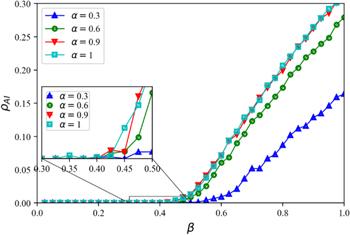
Figure 5. ${\rho }_{AI}$ as a function of the disease transmission rate $\beta $ under different activity level $\alpha $ in the information diffusion layer. Dynamical parameters: information layer spreading rate $\lambda =0.4$ and information forgetting rate $\sigma =0.4,$ disease recovery rate $\mu =0.6,$ infection reduction factor $\phi =0.5,$ active level of nodes in the disease transmission layer $\omega =0.4.$
Next, we explore the impact of individual activity $\omega $ in the disease transmission layer on disease transmission, and related results are shown in figures 6 and 7.
Figure 6. Stationary state and critical threshold of the disease with different spreading rate $\lambda ,$ $\beta .$ Activity level $\omega $ in the disease transmission layer is set as follows: (a) $\omega =0.3,$ (b) $\omega =0.6,$ (c) $\omega =0.9,$ from left to right. Color maps represent the prevalence of the disease. The dotted line represents the threshold ${\beta }^{c},$ and the solid line represents the threshold ${\beta }^{{c}^{^{\prime} }}$ predicted by the model. Each point in grid 40 * 40 in the figure is obtained through an average of 50 numerical simulations. Dynamical parameters: information forgetting rate $\sigma =0.4,$ disease recovery rate $\mu =0.6,$ infection reduction factor $\phi =0.5,$ active level of nodes in the information diffusion layer $\alpha =0.4.$
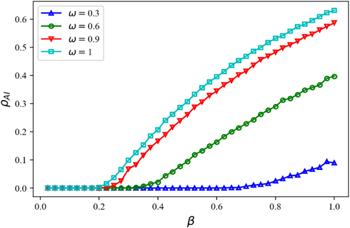
Figure 7. ${\rho }_{AI}$ as a function of the disease transmission rate $\beta $ under activity level $\omega $ in the disease transmission layer. Dynamical parameters: information diffusion rate $\lambda =0.4$ and information forgetting rate $\sigma =0.4,$ disease recovery rate $\mu =0.6,$ infection reduction factor $\phi =0.5,$ active level of nodes in the information diffusion layer $\alpha =0.4.$
From equation (31), we can see that the activity of nodes in the disease transmission layer has a certain impact on the threshold of disease transmission. Secondly, figures 6 and 7 depict the effect of different activity levels of nodes on disease transmission, as well as disease thresholds in the disease transmission layer. In figure 6, We carry out a heat map of the final scale of the disease under different activity levels $\omega $ and different information diffusion probabilities $\beta $ of the node, which exhibits obvious critical phenomenon. Consistent with figure 4, the effect $\lambda $ has on the transmission threshold of disease can be classified into two categories, of which one is the dotted line that represents the threshold ${\beta }^{c}$ and the other is the solid line that denotes the threshold ${\beta }^{{c}^{^{\prime} }},$ which is predicted by the model. In figure 6, the final size of the disease transmission is indicated by the color depth. The darker the color, the easier the disease transmission, and the lighter the color, the harder the disease transmission. In this case, compared with figures 6(a), (b) and (c), the increase in the activity level of individuals will promote the transmission size of the disease, and the threshold of the disease transmission will be decreased, which has a great impact on the transmission size of the disease. Figure 7 shows the effect of individual activity level $\omega $ on disease transmission in the disease transmission layer. We can see that the final size of ${\rho }_{AI}$ and the threshold of disease transmission are significantly affected by the activity level of individuals in the disease transmission layer. In fact, reducing people’s activity level in the physical contact layer is an effective means to control the spread of disease.
In figure 8, we consider that the difference in the effect of $\omega $ and $\alpha $ on disease transmission. We may obtain the conclusion that $\omega $ has a greater impact on disease transmission than $\alpha $ during disease outbreaks. This is consistent with the results of our previous research, which proves the effectiveness of the model and simulation. Therefore, in the face of disease outbreaks, the government should focus on limiting personal behavior (such as wearing masks when going out, keeping a distance when eating in the store, etc).
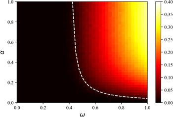
Figure 8. The heat map under the joint action of individual behavior rate $\alpha $ of the information diffusion layer and individual behavior rate $\omega $ of the disease transmission layer. The remaining parameters are set to be: information diffusion rate $\lambda =0.4$ and information forgetting rate $\sigma =0.4.$
Figure 9 describes the heat map of the final scale of the disease under different infection reduction factor $\phi $ and disease transmission rate $\beta .$ We find that when the disease transmission rate $\beta $ remains unchanged, the higher the value $\phi ,$ the more prevalent the disease.
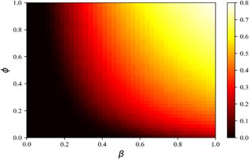
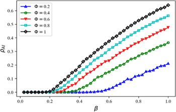
Figure 9. The heat map shows the impact $\phi $ (infection reduction factor when a susceptible individual is aware of the disease) on disease transmission. The remaining parameters are set to be: information diffusion rate $\lambda =0.4$ and information forgetting rate $\sigma =0.4,$ disease recovery rate $\mu =0.6,$ activity level on the information diffusion layer $\alpha =0.3,$ activity level on the disease transmission layer $\omega =0.3.$
In figure 10, we consider the final size of spreading dynamics ${\rho }^{AI}$ in case of different combinations of disease transmission rate $\beta $ and infection reduction factor $\phi .$ There is no doubt that the greater the value of $\phi ,$ the less an individual is aware of the disease-related information. Therefore, the individual behavior of disease prevention will be decreased, the smaller the threshold of disease transmission, and the easier the disease transmits. This conclusion is consistent with that in figure 9, which verifies the correctness of our experiment. During disease (for carrier-dependent infectious diseases, like cholera, diarrhea, etc) outbreak [40, 41], the government can increase the publicity of disease-related information, which will improve the individual’s awareness of the disease and then strengthen the disease prevention measures.
Figure 10. The final size of spreading dynamics ${\rho }^{AI}$ with different disease transmission rate $\beta $ and infection reduction factor $\phi .$ The remaining parameters are set to be: information diffusion rate $\lambda =0.4$ and information forgetting rate $\sigma =0.4,$ disease recovery rate $\mu =0.6.$

5. Conclusion

In this paper, the improved $\mathrm{UAU}\unicode{x02013}\mathrm{SIS}$ model with asymmetric activity of individuals on a multiplex network is established, the upper network represents the diffusion of disease-related information, and the lower network denotes the transmission of disease. Then the system dynamics equations and the critical threshold of the model are determined by using the micro-Markov Chain method. Finally, the correctness of the theoretical analysis is verified by numerical simulation. It is concluded that the asymmetric activity of individuals in the information transmission layer and disease transmission layer has different effects on disease transmission. The activity of individuals in the physical contact layer greatly affects the scale and threshold of disease transmission, but the role in the virtual information layer is not obvious. Therefore, during the outbreak of disease, on the one hand, the government should restrict individual behavior (such as wearing masks when going out; restricting or stopping fairs, theater performances, or other crowd gathering activities, etc); on the other hand, since individual awareness will affect individual behavior, the government should positively carry out online education activities to expand people’s acquaintance with disease-related knowledge.

Conflict of interest

The authors have no conflicts to disclose.

Author contributions

XX, Methodology (equal); Software (equal); Visualization (equal); Writing—original draft (equal). LH, Funding acquisition (supporting); Investigation (Lead); Supervision (Lead); Writing—original draft (Lead); Writing—review and editing (equal). LZ, Investigation (Lead); Supervision (Lead). YQ, Supervision (Lead).

Appendix A

$\begin{eqnarray}{r}_{i}=\alpha {r}_{i}^{m}+\left(1-\alpha \right){r}_{i}^{n}=\alpha {\left(1-\lambda {\theta }_{1}{\rm{\Delta }}t\right)}^{k}+\left(1-\alpha \right){\left(1-\alpha \lambda {\theta }_{1}{\rm{\Delta }}t\right)}^{k},\end{eqnarray}$
$\begin{eqnarray}\begin{array}{c}{q}_{i}^{A}=\omega {q}_{i}^{A,a}+\left(1-\omega \right){q}_{i}^{A,d}\\ \,=\,\omega \alpha {\left(1-{\theta }_{2}{\beta }^{A}{\rm{\Delta }}t\right)}^{l}+\omega \left(1-\alpha \right){\left(1-\alpha {\theta }_{2}{\beta }^{A}{\rm{\Delta }}t\right)}^{l}\\ \,+\,\left(1-\omega \right)\alpha {\left(1-{\omega }^{2}{\theta }_{2}{\beta }^{A}{\rm{\Delta }}t\right)}^{l}+\left(1-\alpha \right)\left(1-\omega \right){\left(1-{\omega }^{2}{\theta }_{2}{\beta }^{A}{\rm{\Delta }}t\right)}^{l},\end{array}\end{eqnarray}$
$\begin{eqnarray}\begin{array}{c}{q}_{i}^{U}=\omega {q}_{i}^{U,a}+\left(1-\omega \right){q}_{i}^{U,d}\\ \,=\,\omega \alpha {\left(1-{\theta }_{2}{\beta }^{U}{\rm{\Delta }}t\right)}^{l}+\omega \left(1-\alpha \right){\left(1-\alpha {\theta }_{2}{\beta }^{U}{\rm{\Delta }}t\right)}^{l}\\ \,+\,\left(1-\omega \right)\alpha {\left(1-{\omega }^{2}{\theta }_{2}{\beta }^{U}{\rm{\Delta }}t\right)}^{l}+\left(1-\alpha \right)\left(1-\omega \right){\left(1-{\omega }^{2}{\theta }_{2}{\beta }^{U}{\rm{\Delta }}t\right)}^{l},\end{array}\end{eqnarray}$

At time $t+{\rm{\Delta }}t,$ the number change rates of the three primary states are denoted as:

$\begin{eqnarray}\begin{array}{l}US\left(k,l,t+{\rm{\Delta }}t\right)=US\left(k,l,{\rm{\Delta }}t\right)-US\left(k,l,{\rm{\Delta }}t\right)\left(1-{r}_{i}\right)\\ \,-\,US\left(k,l,t\right)\left(1-{q}_{i}^{U}\right)+\delta {\rm{\Delta }}tAS\left(k,l,t\right),\end{array}\end{eqnarray}$
$\begin{eqnarray}\begin{array}{l}AS\left(k,l,t+{\rm{\Delta }}t\right)=AS\left(k,l,{\rm{\Delta }}t\right)-AS\left(k,l,{\rm{\Delta }}t\right)\left(1-{r}_{i}\right)\\ \,-\,AS\left(k,l,t\right)\left(1-{q}_{i}^{A}\right)+\delta {\rm{\Delta }}tAS\left(k,l,t\right)+\mu {\rm{\Delta }}tAI\left(k,l,t\right),\end{array}\end{eqnarray}$
$\begin{eqnarray}\begin{array}{l}AI\left(k,l,t+{\rm{\Delta }}t\right)=AI\left(k,l,{\rm{\Delta }}t\right)\left(1-{q}_{i}^{{\rm{U}}}\right)\\ \,-\,AS\left(k,l,t\right)\left(1-{q}_{i}^{{\rm{A}}}\right)+\mu {\rm{\Delta }}tAI\left(k,l,t\right).\end{array}\end{eqnarray}$

From equation (A.1), (A.2) and (A.3). Omitting the higher-order infinitesimal, we can obtain:

$\begin{eqnarray}1-{r}_{i}=\left(2\alpha -{\alpha }^{2}\right)\lambda k{\theta }_{1}{\rm{\Delta }}t,\end{eqnarray}$
$\begin{eqnarray}\begin{array}{l}1-{q}_{i}^{A}\\ \,=\,\omega \alpha \left(2-\alpha +2\omega -2{\omega }^{2}-\alpha \omega +\alpha {\omega }^{2}\right)l{\theta }_{2}{\beta }^{A}{\rm{\Delta }}t,\end{array}\end{eqnarray}$
$\begin{eqnarray}\begin{array}{l}1-{q}_{i}^{U}\\ \,=\,\omega \alpha \left(2-\alpha +2\omega -2{\omega }^{2}-\alpha \omega +\alpha {\omega }^{2}\right)l{\theta }_{2}{\beta }^{U}{\rm{\Delta }}t.\end{array}\end{eqnarray}$

From equations (A.4A.6) and condition ${\rho }^{US}(k,l,t)+{\rho }^{AS}(k,l,t)+{\rho }^{AI}(k,l,t)=1,$ when ${\rm{\Delta }}t\to 0,$ we can get:

$\begin{eqnarray}\left\{\begin{array}{c}\displaystyle \frac{\partial {\rho }^{US}\left(k,l,t\right)}{{\rm{d}}t}=-\left(2\alpha -{\alpha }^{2}\right)\lambda k{\theta }_{1}\left(k,l,t\right){\rho }^{US}\left(k,l,t\right)\\ \,-\,\omega \alpha \left(2-\alpha +2\omega -2{\omega }^{2}-\alpha \omega +\alpha {\omega }^{2}\right){\beta }^{U}l{\theta }_{2}\left(k,l,t\right){\rho }^{US}\left(k,l,t\right)\\ \,+\,\delta {\rho }^{US}\left(k,l,t\right),\\ \displaystyle \frac{\partial {\rho }^{AS}\left(k,l,t\right)}{{\rm{d}}t}=\left(2\alpha -{\alpha }^{2}\right)\lambda k{\theta }_{1}\left(k,l,t\right){\rho }^{US}\left(k,l,t\right)\\ \,-\,\omega \alpha \left(2-\alpha +2\omega -2{\omega }^{2}-\alpha \omega +\alpha {\omega }^{2}\right){\beta }^{A}l{\theta }_{2}\left(k,l,t\right){\rho }^{AS}\left(k,l,t\right)\\ \,+\,\delta {\rho }^{AS}\left(k,l,t\right)+\mu {\rho }^{AI}\left(k,l,t\right),\\ \displaystyle \frac{\partial {\rho }^{AI}\left(k,l,t\right)}{{\rm{d}}t}=\omega \alpha \left(2-\alpha +2\omega -2{\omega }^{2}-\alpha \omega +\alpha {\omega }^{2}\right)l{\theta }_{2}{\beta }^{U}(k,l,t){\rho }^{US}(k,l,t)\\ \,+\,\omega \alpha \left(2-\alpha +2\omega -2{\omega }^{2}-\alpha \omega +\alpha {\omega }^{2}\right){\beta }^{A}l{\theta }_{2}\left(k,l,t\right){\rho }^{AS}\left(k,l,t\right)\\ \,-\,\mu {\rho }^{AI}(k,l,t).\end{array}\right.\end{eqnarray}$

Then, order that $\tfrac{\partial {\rho }^{US}\left(k,l,t\right)}{{\rm{d}}t}=0,$ $\tfrac{\partial {\rho }^{AS}\left(k,l,t\right)}{{\rm{d}}t}=0,$ $\tfrac{\partial {\rho }^{AI}\left(k,l,t\right)}{{\rm{d}}t}=0,$ the steady state equation of equation (A.10) can be obtained:

$\begin{eqnarray}\left\{\begin{array}{l}{\rho }^{US}(k,l,\infty )=\displaystyle \frac{-\mu \delta }{\left.\left(\delta \left(\left(2\alpha -{\alpha }^{2}\right)\lambda {\theta }_{1}k-\mu \right)-\left(\left(-2\alpha +{\alpha }^{2}\right)\lambda {\theta }_{1}k-\left(2\alpha -{\alpha }^{2}\right){\beta }^{U}l{\theta }_{2}\left(2\omega -{\omega }^{2}\right)\right)\left(-\delta -\mu -\left(2\alpha -{\alpha }^{2}\right)l{\theta }_{2}{\beta }^{A}\left(2\omega -{\omega }^{2}\right)\right)\right)\right)},\\ {\rho }^{AS}(k,l,\infty )=\displaystyle \frac{\mu \left(\left(-2\alpha +{\alpha }^{2}\right)\lambda {\theta }_{1}k-\left(2\alpha -{\alpha }^{2}\right){\beta }^{U}l{\theta }_{2}\left(2\omega -{\omega }^{2}\right)\right)}{\left(\delta \left(\left({\alpha }^{2}-2\alpha \right)\lambda {\theta }_{1}k-\mu \right)-\left(\left(-2\alpha +{\alpha }^{2}\right)\lambda {\theta }_{1}k-\left(2\alpha -{\alpha }^{2}\right){\beta }^{U}l{\theta }_{2}\left(2\omega -{\omega }^{2}\right)\right)\left(-\delta -\mu -\left(2\alpha -{\alpha }^{2}\right){\beta }^{U}l{\theta }_{2}\left(2\omega -{\omega }^{2}\right)\right)\right)},\\ {\rho }^{AI}\left(k,l,\infty \right)=1-\displaystyle \frac{\left(\mu \left(\delta -\left({\alpha }^{2}-2\alpha \right)\left({\beta }^{U}l{\theta }_{2}\omega \left(1+\omega -{\omega }^{2}\right)+\lambda k{\theta }_{1}\right.\right)\right.}{\left(\delta \left(\left({\alpha }^{2}-2\alpha \right){\beta }^{U}l{\theta }_{2}\omega \left({\omega }^{2}-\omega -1\right)+\mu \right)-\left({\alpha }^{2}-2\alpha \right)\left(\mu +\left({\alpha }^{2}-2\alpha \right){\beta }^{A}l{\theta }_{2}\omega \left({\omega }^{2}-\omega -1\right)\right)\left(\lambda k{\theta }_{1}+{\beta }^{U}l{\theta }_{2}\omega \left(1+\omega -{\omega }^{2}\right)\right)\right.},\end{array}\right.\end{eqnarray}$
And ${\rho }^{A}\left(k,l,t\right)={\rho }^{AS}\left(k,l,t\right)+{\rho }^{AI}\left(k,l,t\right)=1-{\rho }^{US}\left(k,l,t\right),$ Therefore, we have:
$\begin{eqnarray}{\rho }^{A}\left(k,l,t\right)=1-\displaystyle \frac{-\mu \delta }{\left.\left(\delta \left(\left(2\alpha -{\alpha }^{2}\right)\lambda {\theta }_{1}k-\mu \right)-\left(\left(-2\alpha +{\alpha }^{2}\right)\lambda {\theta }_{1}k-\left(2\alpha -{\alpha }^{2}\right){\beta }^{U}l{\theta }_{2}\left(2\omega -{\omega }^{2}\right)\right)\left(-\delta -\mu -\left(2\alpha -{\alpha }^{2}\right)l{\theta }_{2}{\beta }^{A}\left(2\omega -{\omega }^{2}\right)\right)\right)\right)},\end{eqnarray}$

Considering that equation ${\theta }_{1}\left(k,l,\infty \right)=\displaystyle \frac{1}{\left\langle k\right\rangle }\displaystyle {\sum }_{k}P\left(k\right){\rho }^{A}\left(k,l,\infty \right)=f\left({\theta }_{1}\left(k,l,\infty \right)\right.$ and $f\left({\theta }_{1}\left(k,l,\infty \right)\right.$ is strictly monotonically increasing functions, the existence condition of non-zero solutions of ${\theta }_{1}(k,l,\infty )$ is $\displaystyle \frac{{\rm{d}}}{{\rm{d}}{\theta }_{1}}f({\theta }_{1}(k,l,\infty )){| }_{{\theta }_{1}(k,l,\infty )=0}\gt 1$

Then, we can obtain:

$\begin{eqnarray}\displaystyle \frac{\left\langle {k}^{2}\right\rangle }{\left\langle k\right\rangle }\cdot \displaystyle \frac{\left(\left(2\alpha -{\alpha }^{2}\right)\lambda \delta \mu \left(\mu +\left({\alpha }^{2}-2\alpha \right)l{\theta }_{2}{\beta }^{A}\left(-\omega +\left({\omega }^{2}-\omega \right)\right)\right)\right.}{\delta \left(\mu +\left({\alpha }^{2}-2\alpha \right){\beta }^{U}{\theta }_{2}\left(-\omega +\left({\omega }^{2}-\omega \right)\right)+\left({\alpha }^{2}-2\alpha \right){\beta }^{U}l{\theta }_{2}\left(-\omega +\right.\left({\omega }^{2}-\omega \right)\right){\left(\mu +\left({\alpha }^{2}-2\alpha \right){\theta }_{2}{\beta }^{A}l\left(-\omega +\left({\omega }^{2}-\omega \right)\right)\right)}^{2}}\gt 1,\end{eqnarray}$

Then, we can get the disease threshold ${\lambda }^{c}$ as:

$\begin{eqnarray}{\lambda }_{c}=\displaystyle \frac{\langle k\rangle }{\langle {k}^{2}\rangle }\cdot \displaystyle \frac{\delta \left(\mu +\left({\alpha }^{2}-2\alpha \right){\beta }^{U}{\theta }_{2}\left(-\omega +\left({\omega }^{2}-\omega \right)\right)\right.+\left({\alpha }^{2}-2\alpha \right){\beta }^{U}l{\theta }_{2}\left(-\omega +\left({\omega }^{2}-\omega \right)\right){\left(\mu +\left({\alpha }^{2}-2\alpha \right){\theta }_{2}{\beta }^{A}l\left(-\omega +\left({\omega }^{2}-\omega \right)\right)\right)}^{2}}{\left(\left(2\alpha -{\alpha }^{2}\right)\delta \mu \left(\mu +\left({\alpha }^{2}-2\alpha \right)l{\theta }_{2}{\beta }^{A}\left(-\omega +\left({\omega }^{2}-\omega \right)\right)\right)\right.},\end{eqnarray}$

In order to simplify this result, we make:

$\begin{eqnarray}\psi =\displaystyle \frac{\delta \left(\mu +\left({\alpha }^{2}-2\alpha \right){\beta }^{U}{\theta }_{2}\left(-\omega +\left({\omega }^{2}-\omega \right)\right)+\left({\alpha }^{2}-2\alpha \right){\beta }^{U}l{\theta }_{2}\left(-\omega +\left({\omega }^{2}-\omega \right)\right){\left(\mu +\left({\alpha }^{2}-2\alpha \right){\theta }_{2}{\beta }^{A}l\left(-\omega +\left({\omega }^{2}-\omega \right)\right)\right)}^{2}\right.}{\left(\left(2\alpha -{\alpha }^{2}\right)\delta \mu \left(\mu +\left({\alpha }^{2}-2\alpha \right)l{\theta }_{2}{\beta }^{A}\left(-\omega +\left({\omega }^{2}-\omega \right)\right)\right)\right.},\end{eqnarray}$

Finally, we get:

$\begin{eqnarray*}{\lambda }_{c}=\displaystyle \frac{\lt k\gt }{\lt {k}^{2}\gt }\cdot \psi \,(31)\end{eqnarray*}$

The authors are very grateful to the anonymous referees for their valuable comments and suggestions, helping them to improve the quality of this paper. This work was partially supported by the Project for the National Natural Science Foundation of China (72174121, 71774111), and the Program for Professor of Special Appointment (Eastern Scholar) at Shanghai Institutions of Higher Learning, and the Project for the Natural Science Foundation of Shanghai (21ZR1444100), and Project soft science research of Shanghai (22692112600), National Social Science Foundation of China (21BGL217, 22BGL240).

1
Rhee C 2021 Infectious diseases society of America position paper: recommended revisions to the national severe sepsis and septic shock early management bundle (SEP-1) sepsis quality measure Clin. Infect. Dis. 72 541 552

DOI

2
Sun Q 2022 Diffusion of resources and their impact on epidemic spreading in multilayer networks with simplicial complexes Chaos Solit. 164 112734

DOI

3
Fan J 2022 Epidemics on multilayer simplicial complexes Proc. R. Soc. A 478 20220059

DOI

4
Ross R 1911 The Prevention of Malaria. London Murray

5
Anderson R M May R M 1992 Infectious Diseases of Humans: Dynamics and Control. Oxford Oxford University Press

6
Kermack W O McKendrick A G 1927 Contributions to the mathematical theory of epidemics Proc. R. Soc. A 115 700 721

DOI

7
Gray A 2011 A stochastic differential equation SIS epidemic model SIAM J. Appl. Math. 71 876 902

DOI

8
McCluskey cc 2010 Complete global stability for an SIR epidemic model with delay—distributed or discrete Nonlinear Anal. Real World Appl. 11 55 59

DOI

9
Watts D J Strogatz S H 1998 Collective dynamics of ‘small-world’ networks Nature 393 440 442

DOI

10
Barabási A L Albert R 1999 Emergence of scaling in random networks Science 286 509 512

DOI

11
Pastor-Satorras R 2015 Epidemic processes in complex networks Rev. Mod. Phys. 87 925

DOI

12
Jusup M 2022 Social physics Phys. Rep. 948 1 148

DOI

13
Song X Xiao F 2022 Combining time-series evidence: a complex network model based on a visibility graph and belief entropy Appl. Intel. 52 10706 10715

DOI

14
Zhang Z 2020 Reachability analysis of networked finite state machine with communication losses: a switched perspective IEEE J. Sel. Areas Commun. 38 845 853

DOI

15
Li N 2020 Fixed-time synchronization of coupled neural networks with discontinuous activation and mismatched parameters IEEE Trans. Neural Netw. Learn. Syst. 32 2470 2482

DOI

16
Buono C 2014 Epidemics in partially overlapped multiplex networks PLoS One 9 e92200

DOI

17
Alvarez-Zuzek L G 2017 Epidemic spreading in multiplex networks influenced by opinion exchanges on vaccination PLoS One 12 e0186492

DOI

18
Sartori F 2022 A comparison of node vaccination strategies to halt SIR epidemic spreading in real-world complex networks Sci. Rep. 12 21355

DOI

19
Cremonini M Maghool S 2022 The dynamical formation of ephemeral groups on networks and their effects on epidemics spreading Sci. Rep. 12 683

DOI

20
Silva D H Anteneodo C Ferreira S C 2023 Epidemic outbreaks with adaptive prevention on complex networks Commun. Nonlinear Sci. Numer. Simul. 116 106877

DOI

21
Jin Z Duan D Wang N 2022 Cascading failure of complex networks based on load redistribution and epidemic process Physica A 606 128041

DOI

22
Li W 2023 Coevolution of epidemic and infodemic on higher-order networks Chaos, Solitons Fractals 168 113102

DOI

23
Zwilling M 2022 Cyber security awareness, knowledge and behavior: a comparative study J. Comput. Inf. Syst. 62 82 97

DOI

24
Gu J 2023 The influence of individual emotions on the coupled model of unconfirmed information propagation and epidemic spreading in multilayer networks Physica A 609 128323

DOI

25
Xu H Xie W Han D 2023 A coupled awareness—epidemic model on a multi-layer time-varying network. Chaos: an Interdisciplinary J. Nonlinear Sci. 33 013110

DOI

26
Ullah I Ahmad S Zahri M 2023 Investigation of the effect of awareness and treatment on Tuberculosis infection via a novel epidemic model Alexandria Eng. J. 68 127 139

DOI

27
Funk S 2009 The spread of awareness and its impact on epidemic outbreaks Proc. Natl Acad. Sci. 106 6872 6877

DOI

28
Granell C Gómez S Arenas A 2013 Dynamical interplay between awareness and epidemic spreading in multiplex networks Phys. Rev. Lett. 111 128701

DOI

29
Chen J 2023 Asymmetrically interacting dynamics with mutual confirmation from multi-source on multiplex networks Inf. Sci. 619 478 490

DOI

30
Da Silva P C V 2019 Epidemic spreading with awareness and different timescales in multiplex networks Phys. Rev. E 100 032313

DOI

31
Wang W 2016 Suppressing disease spreading by using information diffusion on multiplex networks Sci. Rep. 6 1 14

DOI

32
Pan Y Yan Z 2018 The impact of multiple information on coupled awareness-epidemic dynamics in multiplex networks Physica A 491 45 54

DOI

33
Kotnis B Kuri J 2013 Stochastic analysis of epidemics on adaptive time varying networks Phys. Rev. E 87 062810

DOI

34
Rizzo A Frasca M Porfiri M 2014 Effect of individual behavior on epidemic spreading in activity-driven networks Phys. Rev. E 90 042801

DOI

35
Liu C 2015 Activity of nodes reshapes the critical threshold of spreading dynamics in complex networks Physica A 432 269 278

DOI

36
Fan C 2016 Effect of individual behavior on the interplay between awareness and disease spreading in multiplex networks Physica A 461 523 530

DOI

37
Olinky R Stone L 2004 Unexpected epidemic thresholds in heterogeneous networks: The role of disease transmission Phys. Rev. E 70 030902

DOI

38
Wu Q 2010 Oscillations and phase transition in the mean infection rate of a finite population Int. J. Mod. Phys. C 21 1207 1215

DOI

39
Wu Q Fu X 2016 Immunization and epidemic threshold of an SIS model in complex networks Physica A 444 576 581

DOI

40
Hamza B 2020 SIS multi-regions discrete influenza pandemic model and travel-blocking vicinity optimal control strategy on two forms of patch Commun. Math. Biol. Neurosci. 2020 29

DOI

41
Ghosh M 2004 Modelling the spread of carrier-dependent infectious diseases with environmental effect Appl. Math. Comput. 152 385 402

DOI

Outlines

/